
June 2, 2008 in INFORMS News
Analytica 4.1
SHARE: PRINT ARTICLE: https://doi.org/10.1287/orms.2008.03.17

I experienced my first encounter with the now ubiquitous spreadsheet nearly 20 years ago in engineering school. The introduction changed my life. No longer did I have to write in arcane programming languages, wait for programs to compile or wait hours in queue for printed results to find out if my analytical procedures were working as conceived. The spreadsheet seemed to resolve all my difficulties. Spreadsheets used simple declarations, were easy to comment and provided documentation to others on how a given model was intended to work. Compilations were instantaneous, allowing me to see quickly whether my analytical structure was working according to plan. For me and many other students of engineering and analysis, Fortran was quickly becoming a thing of the past.
But the real world has a way of throwing sand in one’s gears. Leaving engineering school exposed me to the world of complexity not easily analogous to the clinical textbook problems of stylized ballistics problems, cold air Brayton cycles and structural statics. Real problems were often messier and took time to understand and simplify to a requisite level. My Swiss Army spreadsheet began to dull. Often as I worked on codifying a problem, I would realize that certain functional systems needed to be rewritten. Unfortunately, the developing complexity of the model was already causing my model to “crystallize” into the flat plane real estate of the spreadsheet. Changing the wrong stuff meant rewriting large portions of other good stuff.

In addition, almost anyone could use a spreadsheet regardless of training. Consequently, the usual rules of good programming were ignored or unknown altogether. Because of the loose structure of the environment, slapdash models were often released to the wild, virus-like, where they evolved and grew legs. I frequently found variations-on-a-theme spreadsheets used out of the context from that originally intended. Formulas were often replaced with a checkbook style series of numerical values. Constants were frequently hard-coded into expressions with little explanation about their meaning or units of measure. Few standards were followed by users of the sheet.
The copy-paste/drag-copy method of propagating formulas also carried with it the pernicious effect of propagating errors. Cell referencing of formulas made it difficult to audit. Combine this with the penchant to hard-code assumptions into formulas, and the persistence of errors seemed forever out of control and compounding. Just two years ago I discovered an error on the order of magnitude of $200 million in a legacy spreadsheet used by a client for several years (“I guess that explains why our forecasts were always so wrong.”). I am not a man free of his own programming peccadilloes. Just this past winter a particularly complex spreadsheet assignment seemed forever error prone. I could not explain why, even with nearly 20 years of modeling experience and all my insistence on standardized approaches, my spreadsheet seemed to produce what I am convinced were spontaneous errors [1].
In parallel to my use of spreadsheets, I learned more about the modeling process in general as my career advanced. What I found was that modeling was more than just a closed mathematical endeavor. It was a social process as well. Models could help organizations learn and help their constituents develop a shared understanding of a problem at hand. Models help us to ask deeper questions and gain a deeper understanding of the world we live in and the problems we face. I found that models provided a useful language of discourse with people from disparate backgrounds, perspectives and levels of understandings. But complexity reared its ugly head again.As spreadsheet models became more complex, the population of people who actually understood what a given model did became reduced only to the author himself. Working as a group to develop a spreadsheet and maintain consistent understanding of the underlying model became nearly impossible.
Mitch Kapor, co-founder of Lotus Development Corp., the company that spread the Lotus 1-2-3 spreadsheet like so many mold spores, remarks that the spreadsheet is “...the equivalent of a single-cell organism, with plenty of room to evolve” [2]. Indeed it is.
Analytica: Beyond the Spreadsheet
ANALYTICA 4.1, a modeling environment developed and published by Lumina Decision Systems (www.lumina.com), is designed to overcome many of the shortcomings of both spreadsheets and procedural programming languages. Approximately 12 years old, Analytica possesses a wide and mature range of modeling and statistical analysis capabilities. To understand them all requires the manual. Here I explain the features of Analytica that have kept me as an active, enthusiastic and productive user for those past 12 years.
Influence diagrams and hierarchical organization. One of the persistent problems with any modeling environment to the non-authoring user is the “forensic opacity”of the overall flow of logic from the contextual framing of the problem at hand to the fixed assumptions through intermediate calculations to the objective functions. Even the author, who possesses the most familiarity with a model, may get lost in particularly complex expressions within a workbook. The observer does not always see clearly where a specific calculation is used next or why a particular reference to a prior calculation is employed at all unless extensive commenting is included. In fact, within a spreadsheet the only real explicit explanation of logic and its flow through a spreadsheet are the occasional user-supplied comments and the toggled trace precedents and dependents (which don’t always trace correctly, anyway, especially with functions such as OFFSET). Analytica overcomes these problems associated with explicitly revealing a model’s logic by using an extended form of the influence diagram.
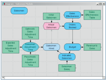
To create the graphical structural elements of a model, a user simply drags an appropriate object node from the tool bar to the palette [Figure 1], which works like a dynamic white board. One can drag-and-drop objects on, move them around or delete them at will.Analytica distinguishes the various nodes of an influence diagram by their shape and color according to their functional use or class. One makes logical connections among nodes by drawing an influence arrow from one variable to another. In this way, the flow of logical precedence and dependence is made obvious to both the user and observer at a primary interface level. This provides another derivative benefit, as well, associated with organizational communication.

To help one avoid accusations of plagiarizing Jackson Pollock’s artwork, Analytica allows you to move collections of variables into modules. Modules function as a subgroup within an overall model and are used to create contextual groupings, store scratch-pad calculations off to a side or group arcane calculations that don’t contribute to the greater level of understanding of a model but are necessary, nonetheless.
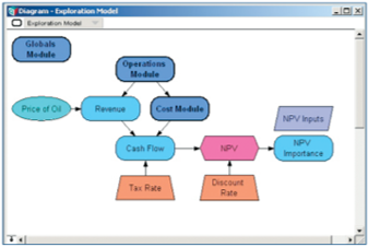
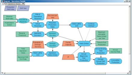
diagram opens up a module that contains a lower layer of detail in a
petroleum exploration model.
For the modeler, debugging and forensic analysis of a model is generally as simple as following the arrows. For the non-authoring contributor or user of a model, understanding the overall flow of logic requires the same level of skill.
Explicit documentation. Every variable or module within an Analytica model is essentially an object with attributes. Among the editable attribute fields are a variable are its title, identifier (the reference used in formulas), units, description, definition (where the actual formulation of a node is written) and userdefined fields as necessary. The object window also displays linkable inputs and outputs to the given variable, providing yet another way to audit the trail of functional performance. To obtain access to this information, one simply double-clicks a node, and its corresponding object window opens.
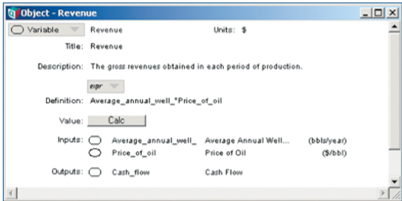
with a variable represented as a node in the influence diagram.
Looking into the object window of a variable reveals a very important aspect of code writing in Analytica – the formulation language is simply an algebraic one. Formulas are created using the identifiers of other nodes. One doesn’t point to a specific value in a table unless one must. In this sense, the benefits of both procedural languages and cell-referencing of spreadsheets are employed.
Intelligent Arrays. One of the most powerful and important aspects of Analytica is its proprietary use of Intelligent Arrays, which is based upon the idea that an index (or a dimension) is an object by itself. But before I explain this feature, recall how tables are currently created in a spreadsheet.
A spreadsheet is a two-dimensional space. Tables are typically composed of row and column headers. The headers are elements across a dimension of concern, and the dimensions are set orthogonally to each other. If one needs to build multidimensional calculations, the tables must either be set in a contiguous arrangement or across multiple sheets. In any case, the larger the tables becomes, the more difficult it is to update and extend the range of row or column dimensions. To compound the difficulties, once the extensions are made, the internal formulas also have to be copied across, further increasing the opportunities for the inclusion and propagation of errors.
In Analytica, indexes represent the analogs of the row and column dimensions of spreadsheets. Each index can either be a numerical sequence or a list of numbers or text elements. These index elements correspond to row and column headers of spreadsheets. Indexes are defined independently of their use within a table; consequently, once an index is made, it can be reused again and again for different calculations or to construct multiple input tables. Indexes are the orthogonal bases of tables, and tables can contain up to 15 indices (essentially, a 15-dimensional hypercube). If an index is extended, the tables on which it is based are also automatically extended, and calculations based on the extended tables or base indexes are appropriately extended as well.
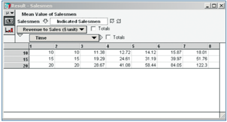
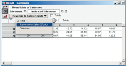
Time. To use all the values in the table at once in another calculation, simply refer to the
identifier of the node that creates this table: Salesmen. If you only need one side of the
table, say the $15/unit plane, use a named reference, like Salesmen [Revenue_to_sales
=15], or a positional reference, like Slice(Salesmen, Revenue to sales, 2.
When one needs to reference subsets or slices of arrays, Analytica uses both a positional and a named reference approach to get at the required data. In spreadsheets, one spends a lot of time writing non-obvious code with INDEX, MATCH, OFFSET and ADDRESS for these types of exercises, or falls back on error-prone specification of individual cell references. One can almost forget being sure if the code is correct if the arrays are multidimensional. In Analytica, if one confirms that the code is right in a couple cases, it is most likely right for the entire array.
The capability for this latter feature derives out of Analytica’s employment of array abstraction.Array abstraction allows a modeler to operate mathematically on an entire table without writing formulas that reference each element in a table or without writing procedural iteration routines, unless specific individual cell references are necessary. Operations across tables take place on a cell-by-cell basis, with the array abstraction logic supplying index values as required. For example, a scalar operation on a table preserves the indices. Operations among tables composed of the same dimensions line up the operations along the same indexes. And operations among tables composed of different indexes increase the dimensionality of the result as the union of the indexes with the operations occurring in the expected tuple-to-tuple manner. The several beneficial results are that time to write code is significantly reduced, copying errors are significantly reduced, and debugging time is reduced. In fact, the size and length of spreadsheets or procedural language models are typically reduced by one to two orders of magnitude [3]. I estimate that the time I spend writing Analytica models is one quarter to one half of that devoted to similarly complex spreadsheets. The ultimate benefit for modelers of sufficient experience is that their efficiency in converting conceptual analysis into results is greatly increased.
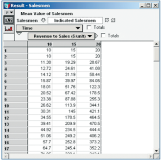
and choose the name of the index to replace the current header.
The bottom table shows the upper table flipped around.
Dynamic simulation. The traditional influence diagram convention requires that the arcs in the node-to-node flow of logic imply a time-forward-only process. For the most part, Analytica follows this convention, but it also allows for a powerful twist: feedback loops are permitted and handled in a logical manner. Modelers are not just constrained to writing static, closed-form formulas as long as at least one of the formulas possesses a time-lagged reference to itself or some other formula within the loop. This permits modeling of time-based dynamic systems without having to learn a special new language of stocks and flows associated with other dynamic system simulation environments or using before- and end-state rows and columns in a spreadsheet.
(Mostly) instantaneous results. Every decision involves a trade-off. The decision to use a spreadsheet allows for numerical expression almost instantaneously (regardless of whether the expression is even right), but logical structure is hidden from immediate view. Logic must be inferred from analysis of cell references and commenting, if the latter is supplied. Analytica takes the opposite route, opting instead to make logical flow and expression explicit while requiring numerical expression to be called. Most of the time, calculation is essentially instantaneous, but there are some caveats to be aware of related to large data structures.
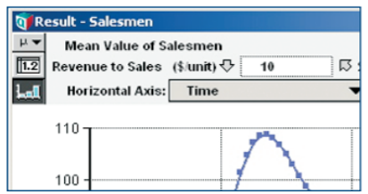
of Jay W. Forrester’s sales effectiveness model discussed in
“Principles of Systems.” The gray arrows indicate dynamic feedback.
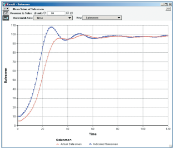
The bottom chart demonstrates that the formulation has captured
the essence of a dynamic response.
Again, Analytica flexes its muscles in the way it presents results. The user can opt to see results in tabular format (like a spreadsheet) across a number of preset statistical options or in graphical format. The leverage of Intelligent Arrays allows a user to pivot and navigate multi-dimensional outputs around the resultant base indexes similar to the way pivot tables are intended to operate,but Analytica’s approach is more logically transparent and instantaneous.
Embedded Monte Carlo. Including probabilistic simulation in spreadsheets often requires the use of third-party plugins. But problems lie here as well. For example, not all spreadsheet models that employ plug-ins work consistently across different versions of the plug-in that may be present among the different analysis and planning departments of a company. Furthermore, plug-ins provide only partial access to commonly useful intermediate statistics. Consequently, the analyst must often resort to supplying another layer of programming to get to these statistics.
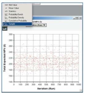
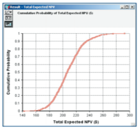
Analytica installs with a fully embedded Monte Carlo engine instead of relying on separate plug-ins. In Analytica, variables used to model uncertainty simply call the required functional distribution (whether one supplied by the system or one provided as a user-defined function), and the user provides either functional links or explicit quantities to satisfy the parameters required by the function. After the call to calculate, if a user needs to see the sample space of a given simulation, he simply switches to the Sample view. Other commonly useful statistics (mid, mean, statistics, probability bands, probability density, cumulative probability,sample) are also available by switching to the appropriate view, but if needed, a full suite of statistical functions are available for more advanced analysis. Unlike many plug-ins, the simulation engine is backward compatible with all prior versions of Analytica.
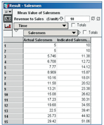
data content can be instantaneously switched back and
forth by clicking the table or graph buttons in the upper
left corner of the result. In this case, the Salesman graph
above reveals its numerical basis.
Because the results of simulation are also expressed in terms of Intelligent Arrays, each uncertain node is capable of producing samples of a desired distribution independently along a given index element.
Connection to data sources. Analytica doesn’t stand alone and isolated from the data warehoused in disparate resources. Analytica can publish data to and subscribe to data from one’s favorite Office applications (let’s be honest, no one really has a favorite Office application, but there may be one that you use mostly for reporting) through OLE to maintain published reports. The Enterprise version of Analytica can use grab data from or push data to existing ODBC-enabled databases through SQL commands for further processing and distribution. In this way, Analytica can work quite well to enhance the use of an organization’s existing spreadsheets as opposed to replacing them. In fact, spreadsheets can continue to be used as effective resources for data collection.
Organizational communication. Analysis conducted within group efforts often experience delays in both development and shared understanding of the implications of the models employed to gain insights into problems. Typically, after problem framing, an analyst goes off to his coding cave where development ensues along with the steps of quality assurance, debugging, and translation of results to a portable format. Once results are observed and discussed, the process may go through several iterations. In my own consulting work with Analytica, I have been able to productively map out and code large sections of models with clients in session. The most successful engagement of this sort occurred with BechtelSAIC [4] in which the analysis team produced a very complex fee adequacy model in a fraction of the estimated time proposed for development with spreadsheets and a Monte Carlo plug-in. While in such working sessions, we were able to get immediate feedback on the logical progression of the model, as well as bring everyone on the analysis team to a similar degree of understanding of how the actual nutsand-bolt of the model worked. This provided a reasonable degree of insurance against failing to meet the modeling goal due to a possible force majeure departure of the primary modeler. I do not think this would have been possible in many other environments other than Analytica’s graphical influence diagram and hierarchical interface.
Beyond promoting analysis team understanding, Lumina provides several avenues to share the insights to be derived from one’s modeling efforts with those who are not yet Analytica users: Player and Power Player, Analytica Decision Engine and the forthcoming Analytica Web Publisher.
The simplest means is to distribute the free Analytica Player or Power Player. Both of these versions allow non-modelers to view model logic, make changes to the inputs and observe outputs. The more basic Player version does not allow persistent changes to inputs between user sessions. The Power Player preserves input changes between working sessions as well as maintains the Enterprise-level features of the most advanced desktop version of Analytica [5].
The Analytica Decision Engine (ADE) is a server application that provides connectivity through Web browser interfaces or other applications to Analytica models and databases. With this “glueware,” an organization can create and distribute custom-made applications that support operations, sales, engineering and planning groups.
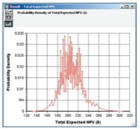
Figures 12, 13 and 14: A robust Monte Carlo engine
provides the samples for simulations. Clicking the
uppermost button in the upper left corner of a
result window provides access to a number
of ways to view statistical interpretations of data.
Clicking the table button reveals the underlying
numerical data.
The latest advancement in ADE technology is the Analytica Web Player. With this tool, models developed in Analytica can be published immediately to a Web browser through a Shockwave GUI. The Web Player exposes all of the features of the desktop model (e.g., influence diagram, object windows, functional inputs, tabular and graphical outputs) to a subscribing user who has to know little more than how to follow arrows, point and click in order understand and use a model.
A Few Caveats
There are a few issues to be aware of as one begins to use Analytica. The ease with which Analytica permits model building often opens the door to the exuberant addition of complexity. The inclination to introduce more complexity than is warranted has to be resisted. Follow Einstein’s dictum: “[models] should be as simple as possible, but no simpler.”
Conceptual complexity presents its own problems, but in Analytica, high-dimensional complexity (i.e, nodes composed of more than three indexes) and large index sizes can cause memory and PC processing resources to be taxed to the limit of standard PC capacities. These limitations can often be overcome with proper problem framing and model planning, but just in case, it helps to have as much RAM as possible. The faster one’s processor performs, the better, too. If the data structures in one’s model do not fit into available RAM, an attempt to calculate will generate an error message. In previous versions, the software would hang. Analytica does give some support to working around memory management problems, but this can be tiresome at times. Unfortunately, there is probably no clean seamless solution to this problem, without substantial compromise to the tool’s functionality.
Lumina recently improved Analytica’s graphing capabilities; however, there are many types of graphs that are available in common spreadsheets that are not yet available in Analytica. Of course, many of these graph variations in spreadsheets are simply chart junk, but if one must be used, the data can always export to a spreadsheet (or your favorite graphing software) where the graph variants can be produced as desired.
Conclusion
Feral spreadsheets will likely always run amok, if for no other reason than almost anyone can plug numbers into an open spreadsheet. The same might be said of Analytica, but at least a modicum of training is required to implement the simplest of Analytica models. Many of the shortcomings of spreadsheets can be overcome within organizations by implementing consistent design procedures and standards. Similar standards should be employed within any modeling environment, including Analytica.
Analytica will not solve all the issues associated with modeling or make every model perfectly transparent to all observers. But it does provide tremendous advancements over the current state of affairs. By providing a more transparent depiction of model logic through the use of influence diagrams, model logic can be audited quickly as well as communicate model rationale to broader audiences. Analytica also reduces the programming effort required to produce insights through its use of Intelligent Arrays, array abstraction and integrated Monte Carlo engine. As a result, analysts are freer to focus more on model exploration and its implications than writing code. In conclusion, if you want to evolve a step beyond your current model development and quality assurance time requirements, error rate and auditable transparency issues associated with spreadsheet and procedural language models, Analytica provides a great environment to do so.
VENDOR'S COMMENTS
Editor’s note: It is the policy of OR/MS Today to allow developers of reviewed software an opportunity to clarify and/or comment on the review article. Following are comments by Max Henrion, chief executive officer, Lumina Decision Systems
We appreciate the reviewer’s enthusiasm for Analytica. His experience that he can develop Analytica models in a quarter to half the time needed for spreadsheets of equivalent complexity is in line with what other users tell us.
In response to the reviewer’s caution that it is easy to make Analytica models so large that they exhaust computational resources, we would add that its Intelligent Arrays features also make it much easier than other modeling tools to vary the level of detail and so adapt the model size to computer resources available. For example, you can easily extend or reduce an index (dimension) of a model – say, change the time horizon, or change aggregation between months, quarters or years, or change8 geographic regions – without having to change formulas that work over those indexes. You can also easily add or remove indexes from an array. In this way, you can actually do sensitivity analysis to see how the level of detail affects precision, and so choose the most appropriate level of aggregation – something that is impractical with spreadsheets or conventional modeling languages.
REFERENCES
1. Raymond Panko provides an excellent discussion on the frequency of spreadsheet errors and their causes in his paper, “What We Know About Spreadsheet Errors,” http://panko.shidler.hawaii.edu/SSR/Mypapers/what know.htm.
2. Scott Leibs, 2003, “Spreadsheets forever: On the eve of its silver anniversary, the electronic spreadsheet remains golden, co-creator Dan Bricklin explains why,” CFO: Magazine for Senior Financial Executives, Fall 2003, http://findarticles.com/p/articles/mi_m3870/is_12_19/ai_108198588.
3. Morgan, M. Granger, and Henrion, Max, 1990, “Analytica: A Software Tool for Uncertainty Analysis and Model Communication Uncertainty in Quantitative Risk and Policy Analysis,” chapter 10 of “Uncertainty: A Guide to Dealing with Uncertainty in Quantitative Risk and Policy Analysis,” Cambridge University Press, New York, reprinted in 1998.
SHARE: