Redistricting, Gerrymandering and the Binomial Distribution

With the completion of the 2020 U.S. Census, due to changes in population totals, many states have had to redraw their legislative voting districts. Most often, the party with the current majority gets to draw the new district lines, although some states have Independent Redistricting Commissions that are intended to turn the work over to a nonpartisan group of experts.

Of course, redistricting is about power. Traditionally, the party drawing the lines wants, first, to maintain the party’s majority in the legislature and, second, to maintain individual incumbency, not just for themselves but also, in some cases, for their friends in the other party.

Beyond those two concerns, the geographic design of districts, of course, has racial, ethnic and/or religious power implications. This article does not directly consider those individual or specific concerns here. Instead, it folds them collectively into party politics and voting.

Redistricting

Redistricting is a complicated process, the result of which generally leads to predictable outcomes for many district elections. There have been many attempts to find a foolproof mathematical procedure for identifying cases of outlandish gerrymandering [1], the most often noted is the “wasted votes” method and the “lopsided margins” test [2]. Those methods are good techniques to indicate “cracking” or “packing,” two common gerrymandering techniques. Neither, however, provides hard and fast limits to indicate if exceptional gerrymandering exists [3]. This article proposes just such a procedure.

Percentage Votes/Seats Won Differences Method

It would seem fair to assume that in a representative form of government, the percentage of legislative seats won by a party should be close to the overall percentage of the vote won by candidates of that party. The most critical question is: Did one party get far more seats in the legislature than the popular vote would indicate? More specifically: Is the difference in the two percentages significant to indicate that some form of voting district gerrymandering had taken place?

Using a data set of state legislature elections [4], the actual relationship between the two percentages can be plotted. The data set included most state legislative elections since 1973. The data included the party vote and number of seats won by each party in each state for each election year. The data set included 806 statewide elections. Every state except Louisiana was included at least once, some as many as more than a dozen times.

Using that state legislative voting data, the graph in Figure 1 shows a strong linear relationship (r-square of 0.81) between the percentage of the statewide vote one party got versus the percentage of seats won. The slope of the line (1.479) indicates that every one percentage point increase in the popular vote results in an increase in the percentage of seats won by approximately 1.5.   

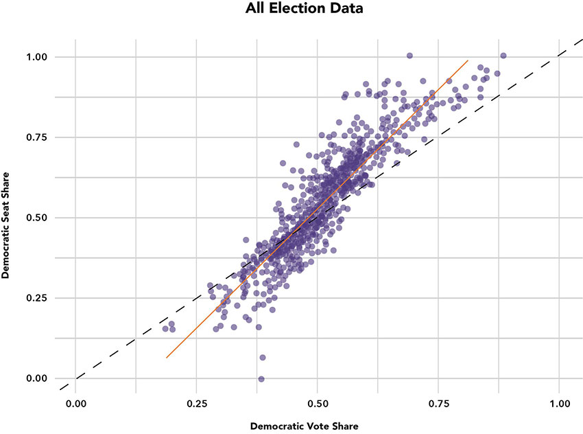
Not all elections fall exactly on the line. It appears that there are a number of outliers that might be indicative of gerrymandering. Note that the vertical variability is quite large. For elections with a popular vote percentage slightly above 50%, the percentage of seats won ranges from around 45% to nearly 75%.

Because voting in most cases is a binary choice, it is worth contemplating whether the binomial distribution can shed some light on what is a reasonable discrepancy between the two percentages and how much is the result of either intentional or unintentional gerrymandering.

The Binomial Model

Consider the following: Assume that, in a democracy, the percentage of seats won is close to the percentage of the statewide popular vote. Assume that the districts are fairly drawn such that each district presents essentially the same probability of victory for one of the parties and that that probability is directly related to the total statewide popular vote percentage. Then, the expected value and variance of seats won are calculated using the binomial distribution, and a 95% confidence interval to predict the statistically reasonable range (an upper and lower limit) of how many seats a party can reasonably be expected to win is calculated. An actual election result outside of that interval may indicate the presence of a substantial amount of gerrymandering. [Note: It does not detect the gerrymandering of one or a few districts.]

Using that approach, Table 1 displays the theoretical maximum number of legislative seats fairly won within a 95% confidence level (2.5% on each tail) given the total seats available (on the left side of the table) and given the percentage of popular vote that a party received (along the top of the table.) For example, in a legislature with 100 seats, it would be statistically reasonable for a party that received 55% of the statewide vote to win up to 65 seats, but not more. Or, in a legislature of 50 seats, it would be statistically reasonable for a party that won 50% of the statewide popular vote to win up to 32 of the 50 seats, but not more.

Table 1. Vote Percent/Seat Percent Comparison: Upper Limits

Due to the nature of the binomial distribution, the limit is not a constant percentage of the total number of seats. As can be seen, the limit varies according to both the vote percentage and size of the legislature. The upper limit for a 10-seat legislature with a 50% popular vote is eight seats (80% of the total), but the limit for a 100-seat legislature with 50% is 60 (only 60% of the total).

Table 2 lists the lower limit of seats that would be reasonable to expect given the popular vote percentage and number of seats in the legislature.

Table 2. Vote Percent/Seat Percent Comparison: Lower Limits

This table indicates that for a legislature of 100 seats, a party that received 55% of the popular vote should get no fewer than 45 seats. Clearly, it is statistically reasonable that they may not get the majority of seats even though they have majority of the popular vote, but not fewer than 45. For that same legislature, a party that received at least 60% of the popular vote should absolutely expect to gain at least a share of the majority, at least 50 of the 100 seats.

Test of Voting Outcomes

Applying the above theoretical binomial concept to state legislature voting data, the number of seats actually won in each of those 806 statewide legislative elections was compared with the limits calculated from the binomial distribution. In 202 of those elections, the majority party won more seats than the limit, which indicates that the winning party received more than the reasonable number of seats that the binomial rule predicts in approximately 25% of the elections.

There is no way to know how many outcomes of those 202 elections were the result of gerrymandering. However, there have been a number of court cases arguing that gerrymandering was present. In recent years, three states have been accused of gerrymandering sufficiently enough to have court cases rise to the Supreme Court – Wisconsin, Maryland and North Carolina. All three show up as “in violation” of the binomial rule, although they are not necessarily the worst violators. In 2012, North Carolina Democrats received 48% of the popular vote and only 35% of the seats. In 2018, Maryland Democrats received 65% of the vote but won an overwhelming 81% of the seats. In 2018, Wisconsin Democrats received 47% of the vote yet won only 35% of the seats.

For small contests (10 seats), the percentage needed to guarantee a majority is so large (75%) that the test likely might not be useful for most states’ congressional elections. However, in 2012, Pennsylvania Democrats won 50.28% of the statewide popular vote for congressional candidates but won only five of the 18 seats. The “binomial” lower limit for a 20-seat contest with a 50% popular vote is six seats. No wonder claims of gerrymandering made it to the courts.

Percentage Needed to Win Majority

Table 3 displays the minimum popular vote percentage needed to “guarantee” a majority (50%) of the legislative seats given the size of the legislature, using a 95% confidence interval.

Table 3. Minimum Popular Vote Percentage to Guarantee Legislative Seats

According to Table 3, for a 100-seat legislature, a party would have to win at least 60% of the popular vote to, in essence, guarantee a majority of seats. But if they won more than 60% of the popular vote and did not win a majority of seats, gerrymandering may be in play.

Binominal p-values

What if the party wins a higher percentage of seats than their popular vote percentage but fewer seats than the limit? For example, in a 100-seat legislature, what if a party won 50% of the popular vote and won fewer than the 60-seat limit? That doesn’t mean that gerrymandering didn’t exist. It just means it fails the 95% test.

The p-value of the binomial would provide the probability of gerrymandering. Table 4 presents those probabilities for a 100-seat legislature.

Table 4. Probability of Gerrymandering

This provides guidance as to the probability that some form of gerrymandering may have existed even if the limits provided earlier are not violated. Thus, for a 100-seat legislature, what if the party with 50% of the vote won 56 seats? This analysis indicates there is a 90% chance that some form of gerrymandering existed. That may be enough to raise concerns.

Assumptions

Use of the binomial distribution requires that each “trial” has essentially the same probability of “success.” Is it possible to create districts that all have similar success probabilities? Unfortunately, voting patterns tend to be unevenly spread geographically. In most states, voting results tend to be concentrated rather than dispersed. Making districts with similar probabilities may require the creation of districts with very bizarre shapes, precisely what anti-gerrymandering efforts are trying to prevent.

It may be more feasible to design districts so that the number of competitive districts is as high as possible and the remaining noncompetitive districts are divided as equally as possible among the parties.

Also, this analysis uses a 95% confidence level approach, which is a generally accepted statistical standard for making inferences. But it is not unusual to use 90% for a significance test. As previously shown, using a 90% confidence level would lead to smaller intervals, bringing an even larger share of elections into question.

Discussion

Our democracy is really a republic – a representative form of government in which the people choose their leaders. Once elected, those leaders are supposed to represent the “best” interests of their constituents.

What does representation really mean? Does it mean geographic interests (e.g., “Our area needs better roads.”)? Does it mean policy representation (e.g., “All people should have universal healthcare.”)? Does it mean ethnic/racial/religious representation (e.g., “We need a representative who looks like us.”)? No one seems to know precisely.

This article distilled (rightly or wrongly) all of those issues into party choices, primarily because those seem to be the real choices with which we are presented. Perhaps a more complete understanding of representation could lead to a better governmental structure.

Conclusion

This article proposes one more approach to understanding the relationship between the will of the people as expressed by their votes and the resulting power achieved by a party, with the hopes that, in conjunction with other models, it can provide more clarity into this complex problem.

Acknowledgment

I’d like to acknowledge my research assistant, Louis Nix, who is currently a senior analyst at Cinc and received his master’s degree in quantitative methods in the social sciences from Columbia University.

References

1. Michael McDonald, 2019, “The Predominance Test: A Judicially Manageable Compactness Standard for Redistricting,” Yale Law Journal, Vol. 129.
2. Samuel Wang, 2016, “Three Tests for Practical Evaluation of Partisan Gerrymandering,” Stanford Law Review, Vol. 68, No. 6,
3. Lisa Handley, “Some Mathematical Measures for Determining if a Redistricting Plan Disproportionally Advantages a Political Party,” https://tinyurl.com/bdezsujc.
4. Princeton Election Consortium, Princeton University, https://election.princeton.edu