Predictive Analytics: Managing Fundamental Tradeoffs

People love all sorts of “one click” applications because they are easy to handle, but they are like an analog radio that’s pre-tuned to a single station; you won’t find it too useful unless this single station happens to be the only station that you will ever listen to. To allow you to listen to different stations, the radio must come with a knob. But the added flexibility must come with a cost; you must turn this knob carefully – otherwise you will hear nothing but static noise. If you are thinking about delving into predictive analytics or data mining, this common-sense principle is one that you must grasp.

The majority – though not all – of the problems encountered in predictive analytics and data mining can be described as one of using some past data to uncover a hidden relationship between a number of inputs and an outcome. Once uncovered, this relationship can be used to make predictions.

For example, we may have a database of individual voters, perhaps thousands of them. For each voter, the database records his or her age, gender, income, education level, and whether he or she voted for a Republican or a Democratic candidate in the previous presidential election. From such a database, we’d like to uncover a rule, which will allow us to use any voter’s gender, income and education level to predict his or her voting behavior in the next election. Of course, any such rule will be quite imperfect in its ability to make the right predictions all the time, but we can still hope to do better than random guessing, perhaps significantly better.

Algorithms used to uncover such a relationship – for example, neural networks and support vector machines – must be sufficiently flexible. This is because only flexible algorithms can be adapted to the vastly different situations that we encounter in practice. For example, you cannot use a linear algorithm to uncover a hidden relationship that is inherently nonlinear. But, like the analog radio that allows you to tune in to different stations, these flexible algorithms also have “knobs” that you must twiddle. As the user of these flexible algorithms, you must use these “knobs” to control their flexibility; otherwise you will only uncover bogus “relationships” that are both irrelevant and wrong.

Nearest Neighbors

To illustrate this, let’s look at how a very simple algorithm called the K-nearest neighbors (KNN) works. Suppose K=5. To predict how Mark is going to vote in the next election, the KNN algorithm simply looks for Mark’s five-nearest neighbors in our database – the five people in our database whose demographic characteristics (in terms of age, gender, income and education level) are the closest to those of Mark’s. If most of these five people voted Democrat in the previous election, the algorithm predicts that Mark will most likely vote Democrat as well. This is an intuitive idea easily understood by all.

So, where is the “knob” in the KNN algorithm? Not surprisingly, it is the number, K, or the number of neighbors the algorithm looks for when trying to make a prediction. Should we look for five-nearest neighbors or 50-nearest neighbors? What happens if we look for too few neighbors? What if we look for too many?

If we look for too many neighbors, then some of these neighbors will necessarily turn out to be not so similar to Mark. For example, if K=500, then his 500th-nearest neighbor is, by definition, not that near. Allowing far-away “neighbors” to influence our prediction will bias our prediction. After all, the intuitive content of the algorithm is to examine people with similar demographic characteristics. But what if we look for too few neighbors? In this case, all the neighbors will be more or less guaranteed to have a similar demographic profile, but we will not have examined enough cases or used enough information from our database to draw a statistically sound conclusion. Consider the extreme case of K=1. What if Mark’s one-nearest neighbor turns out to be a rather unusual individual in our database? Allowing our prediction to depend entirely upon the behavior of just one individual in the database will cause our prediction to be highly unstable, or to have a big variance.

This simple analysis illustrates a fundamental tradeoff that everyone must face in predictive analytics and data mining, the so-called bias-variance tradeoff. For the KNN algorithm, turning the “knob” in one direction (small K) reduces the bias but inflates the variance of its predictions, whereas turning it in the other direction (large K) reduces the variance but inflates the bias. We must turn this “knob” carefully in order to find the right balance, but there is no universal magi
value to set this “knob” to; the optimal position of the “knob” will depend on the specific situation. This is true for all algorithms, not just the KNN. Blind applications of predictive algorithms without carefully turning these “knobs” are sure to produce bad or even disastrous results. This concludes our first lesson.

Decision Tree and Forests

Another widely used algorithm is called the decision tree. The size of the decision tree is an important “knob” and, like the KNN, it is necessary to control this parameter carefully in order for the decision tree to be effective. In particular, a small tree has high bias and low variance, whereas a big tree has low bias and high variance. Some algorithms will have more than one “knob.”

Instead of using a single decision tree, it was recently discovered that using a collection, or an ensemble, of decision trees often significantly improves prediction accuracy. Basically, each tree makes a preliminary prediction, and a majority vote type of rule is used to produce the final prediction. These ensembles of decision trees are sometimes called, quite appropriately, decision forests. In fact, even though we call them forests, they do not have to be ensembles of decision trees. They can be ensembles of anything, but ensembles of decision trees are the most common.

What’s remarkable about these decision forests is that they are capable of making good predictions even if the sizes of individual trees within the forest are not optimal by themselves. The question is: Does this mean we no longer have to worry about turning “knobs” anymore? If you have ever heard of the saying, “there is no free lunch,” your instincts should immediately tell you that this is too good to be true. This brings us to our second lesson.

To create multiple decision trees from the same database, some perturbations are necessary – otherwise every tree in the forest will be identical, which destroys the whole point of having a forest. The simplest kind of perturbation is to put different weights on every record in the database before building each decision tree. This allows the same data to influence each decision tree differently, and thereby allows the same decision tree algorithm to produce trees that are different from each other.

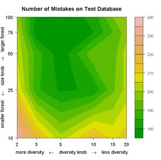
A subtle dilemma now exists. Perturbations are necessary to create different decision trees and form a forest but, on average, they necessarily make each tree less optimal. In 2001, Professor Leo Breiman of the University of California at Berkeley proved mathematically that the best kind of decision forests should consist of very different trees, each capable of making good predictions. That is, we want a diverse collection of strong trees. Unfortunately, actions to increase forest diversity always decrease the average strength of individual trees. For example, one can make the forest more diverse by using stronger perturbations but the stronger perturbations further diminish the strength of each individual tree. Once again, there is a fundamental tradeoff, this time between strength and diversity. Therefore, algorithms to create decision forests usually come with “knobs” as well, ones that allow us to control forest diversity. We want enough diversity, but not too much. Once again, we must turn the “knobs” carefully. Figure 1 shows an example [1] of this tradeoff in action.

Final Lesson

Our third and final lesson is short but no less important. Predictive analytics and data mining are about finding information from data. They are search operations. As with all search operations, there are always two questions: where do we search, and how do we search? The algorithms are concerned with how to search, but we must tell them where to search, that is, we must feed the algorithms with data. These algorithms are both dependent upon and at the mercy of data. If your database contains nothing but junk – for example, if there is no relationship between the inputs and the outcome – you cannot expect any algorithm to find it. The algorithms can only do so much; they cannot perform magic tricks. The quality of your database is crucial. Remember: “Garbage in, garbage out!” Professor Mark van der Laan of the University of California at Berkeley said it well: “We will find you the needle in the haystack, but only if it is actually there.”

A good understanding of these three tradeoffs – bias versus variance, strength versus diversity, where versus how – is critical for successful applications of predictive analytics and data mining. You must control the flexibility of your model. You must control the diversity of your ensemble. You must control the quality of your data. You cannot expect “one click” applications to solve all your problems.

Reference

1. The website www-stat.stanford.edu/~tibs/ElemStatLearn/ contains the databases, and the website http://cran.r-project.org/web/packages/randomForest/ contains the decision forest algorithm used to create this example.