

December 2, 2013 in Five-Minute Analyst
Army-Navy football game
SHARE: PRINT ARTICLE: https://doi.org/10.1287/LYTX.2013.06.13
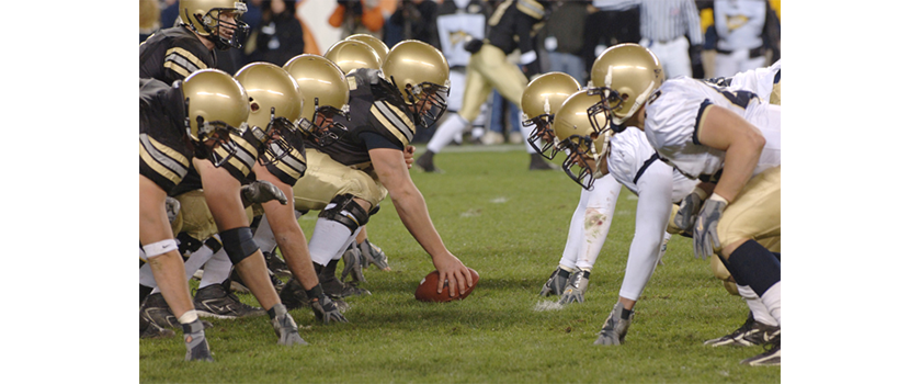
I usually write about fun, lighthearted articles, but now I’m going to write something controversial about an important topic: Army-Navy football. Being a service academy graduate (Navy), I spent a considerable portion of my life wishing for Navy victory; a wish that was denied for four years while I was at the U.S. Naval Academy, but one that has been returned in spades over the past 11 years – Navy is on an 11-game winning streak which began in 2002.
The Army-Navy football game is interesting mathematically in that it is difficult to imagine two long-standing rivals who are as evenly matched. Discussions between alumni (and current students) about the differences between a Navy midshipman and Army cadet really only highlight their similarities: Both met the academies’ rigorous physical, academic and honor standards. Both intend to serve in their respective military branches after graduation. Although there are some notable exceptions, the service academies do not produce many professional athletes.
While both schools boast that they have a superior football team, do they? Analytically speaking, are Army and Navy evenly matched? Consider Figure 1.
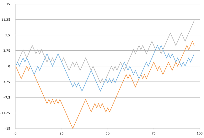
When considering a long-term sum of random variables like Army-Navy game outcomes, it is not sufficient to just ask if the sum of wins and losses is “near” zero. After all, there are other sequences that could result in a sum of zero, such as (-1, +1, -1, +1), etc. If the Army-Navy game were truly a random contest between two well-matched opponents, then we would expect it to be “like” the Random Walk.
The Random Walk is a rich and interesting statistical model. Entire books are devoted to its study, and I will not spoil your fun by trying to go through it in detail here [2]. The idea of the symmetric random walk is a simple one: Imagine flipping a coin; if it comes up “heads,” take one step to the right, and if comes up tails, take one step to the left. This experiment I just described is equally interesting to both elementary school children and graduate students. One of our assumptions is that the conditional probability of the next step is independent of the previous. For our (truncated) historical dataset, this is clearly true:
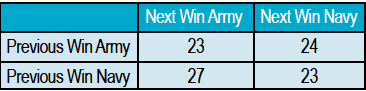
(neglecting current Navy winning streak).
The probability of the next win being Army given the previous win was Army is 49 percent; the probability that the next win will be Navy given the previous win was Navy is 46 percent. Hypothesis testing shows that these values are not inconsistent with an assumed “even” match [3]. However, demonstrating the evenness of the match in this manner is not sufficient to demonstrate randomness; I could construct a deterministic sequence that also had these properties. What I’d really like to do is to consider the probability of the next game’s outcome given all the previous knowledge up to that point across the entire population. I’d also like to do this in an automated fashion with easily interpreted results. In a word, what I want to do is check the data’s autocorrelation. While this can be done in Excel, I have opted to shift to the statistical language R.
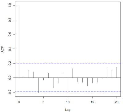
no significant seasonal effect, supporting the hypothesis that the
Army Navy game results are a random process.
We might also consider how the runs of wins and losses affect our estimates of the win probabilities for Navy. We present this for both cumulative history and a 10-game moving average as Figures 3 and 4.
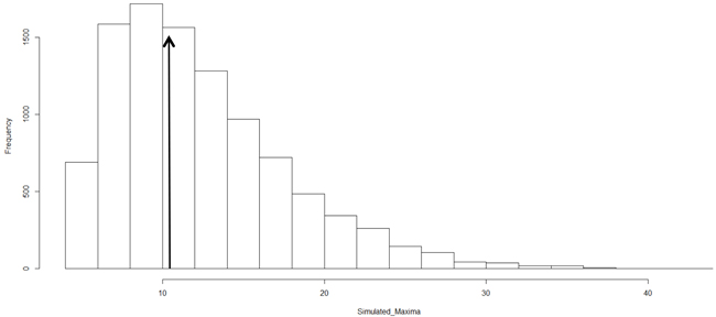
This is all very interesting, but doesn’t much answer our original question, which is: “Are the excursions we see excessive?” This depends greatly on your point of view. There have now been 11 Navy victories in a row; the probability of a fair coin coming up ‘heads’ this many times consecutively is: 1211.?.0005?1:2,000. So from that point of view, the current run is excessive in favor of Navy. However, we could ask this question from a different point of view: What sort of deviation from “even” would be considered excessive? There are many beautiful theoretical results that I might consider if this were written for a different audience. However, this is Analytics, and most of us have to inform decision-makers at the end of our work. This brings up an important optimization problem – the difficulty of briefing an elegant but extraordinarily technical result against simply simulating the problem and providing empirical evidence. For this article, I simulated 10,000 random walks of length 113, and recorded the maximum deviation from zero. The results are shown in Figure 5. The current deviation of 12 is near the midpoint of the distribution – right at the 50th percentile – supporting the claim that over a 113-game history, it is not unusual to see excursions of this size.
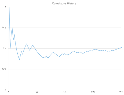
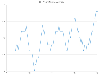
estimated by (L) entire history of the match to that date and
(R) 10-game moving average. While the current Navy winning
streak leads to a moving average of 1 for Navy, there have been
substantial excursions from 50-50 previously. Note that the
cumulative history tends to dilute the deviations
from .5 because of the larger sample size
So, while the current run of 11 wins may be rare, the fact that Navy is currently up by 12 is not, statistically speaking, a rare event in a rivalry of this length.
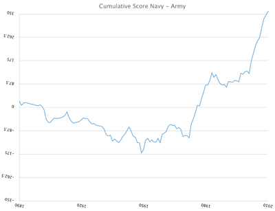
For those who are interested, I have also included a plot of the cumulative score of the football game itself (Figure 6). This plot does not show nearly as much variability as the game outcome (as measured by zero crossings). I include this graph as an interesting picture to think about (and possibly a topic for next November’s FMA)
As far as this year’s football game is concerned, I will be happy with either result. While I can hardly claim neutrality (and my classmates will never let me live it down), I think an Army win this year wouldn’t be such a bad thing – mostly because it would make beating Army more fun the following year.
Editor’s note: The 2013 Army-Navy game will be played Dec. 14 at Lincoln Financial Field in Philadelphia and broadcast live on CBS with a 3 p.m. (ET) kickoff.
References
1. All data is from: http://www.history.navy.mil/special%20highlights/football/army-navy-scores.htm
2. See Brzeznik and Zastawniak, Basic Stochastic Processes, 2003 or similar.
3. p = .57 (2-sided test)
4. max(abs(cumsum(ifelse(runif(n) > .5, 1, -1))))
Harrison Schramm, CAP, PStat, is a senior lecturer at Naval Postgraduate School, splitting his time between Defense Management and Operations Research where, in addition to teaching, he runs the Contested At-Sea Logistics Lab (CASLL). He served as the inaugural chair of the INFORMS Security Conference and is a past president of the INFORMS Analytics Society.
([email protected])