

February 3, 2014 in Five-Minute Analyst:
Markov’s nursery
SHARE: PRINT ARTICLE: https://doi.org/10.1287/LYTX.2014.01.15
This month, we tackle a problem that may be familiar to some readers – the issue of getting multiple young children to sleep. We’ll also use this column to (re)introduce some neat mechanics – the generator matrix. Suppose that a family has two infant children, named Mary and Neil. Now, at bedtime, for analytic purposes, they exist in one of two states: “crying” or “sleeping” [1]. Because there are two children, there are a total of four states that the children could be in: 1. both sleeping; 2. Mary only sleeping; 3. Neil only sleeping; and 4. both crying.
We would like to know the amount of time the system (nursery) spends in each state, particularly the proportion of time both children are asleep. There’s a minor twist to this problem – we assume that if one child is crying, it will reduce the amount of time that the other child is sleeping by half if they are sleeping, or lengthen the amount of time that the other child stays awake if they are currently awake.
There are several approaches we could take to solving this problem. One approach would be to simulate it, another would be to consider the discrete-time, discrete-space Markov chain and compute the limiting distributions the usual way. We’re going to take a different approach, which requires a bit of machinery but ultimately is more straightforward. We’re going to use the generating function of the continuous time Markov Chain, which we (and others!) denote as the G matrix [2].
This matrix differs from the more commonly used P matrix in discrete time chains because it is specified in terms of rates, not probabilities. Have no fear, knowledge of one fundamental matrix implies the other. The practical difference is that the rows of the P matrix sum to 1, while the rows of the G sum to zero, with the on-diagonal elements being negative. For instance, we might specify:
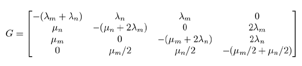
Where  represent the sleeping times of the children, and
  represents their wakeful times. To make use of our model, we need to use P‘t = tG, which is readily solved in matrix form as
P(t) = etG
To evaluate this expression, we need to consider what it means to take e to a matrix power. This turns out not to be any harder than taking ??? to a scalar power – you just have to use Taylor’s Theorem:
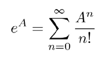
Depending on your programming environment, efficient algorithms exist to compute this numerically.
As an example, if we take  , and recalling that the rate parameters of exponential random variables are the reciprocals of their expectations, we see that Mary is a child who sleeps for 10 hours at a stretch (without interruption from her brother), and Neil is a child who sleeps an average of eight hours at a time. Both infants are up for an average of five hours at a time between sleep stretches. We can use these values to populate the G matrix mentioned earlier.
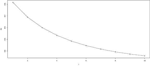
initially asleep. This chart was made by evaluating the matrix exponential at various points
premultiplied by the scalar time, demonstrating the usefulness of this method.
To find the long-run behavior of the system, we choose a value of t which is large enough so that the system is stable but small enough to avoid problems with numerical stability. We select, somewhat arbitrarily, t = 30 to make sure that transients are out of the system. Now, it’s simply a matter of evaluating the expression. We find that in our example that both children are asleep 30 percent of the time, Mary only is sleeping 18 percent of the time, Neil only is sleeping 14 percent of the time, and both children are crying 36 percent of the time. Note that the children do not have equal sleeping behaviors. This is because Mary has a little lambda.
We’ve (somewhat sloppily) found the limiting distribution, but we may do a great deal more. Suppose that both children are currently asleep. We wish to compute the probability that they will still be asleep in one hour. This is easy; we simply compute P(1) = eG and pre-multiply the result by the initial condition vector (1,0,0,0), which strips off the top row, and we see that there is an 81 percent chance that both children will still be sleeping in an hour.
Notes
1. Real children, of course, exist in many states as they grow older.
2. “G Matrix” is another math-rap name ripe for the picking!
Harrison Schramm, CAP, PStat, is a senior lecturer at Naval Postgraduate School, splitting his time between Defense Management and Operations Research where, in addition to teaching, he runs the Contested At-Sea Logistics Lab (CASLL). He served as the inaugural chair of the INFORMS Security Conference and is a past president of the INFORMS Analytics Society.
([email protected])