Herd immunity

Vaccines are important for both individual and public health. INFORMS has a longstanding interest in the topic, with last year’s Edelman Award [1] winners awarded for their work in polio vaccines, as well as a very good TutORial article on the subject [2]. Analytics magazine editor Peter Horner has also written an excellent essay [3] on the personal impacts of preventable polio.

One interesting aspect of vaccination in public health is “herd immunity”; in short, if enough of the population is vaccinated, then individuals who are not vaccinated will be “protected” by the vaccination effect from the rest of the “herd.” The idea is that the force of spread is a function of the number of susceptible individuals the infected individual comes into contact with, and having a large vaccinated population (who are assumed immune) dilutes the infection pressure. This article presents a simple demonstration of this effect, using a deterministic approach. A full treatment requires stochastic methods, which would take far longer than my allotted “five minutes.” An excellent reference for stochastic approaches is Daley and Gani [4].

“Herd immunity” was very much in the public eye because of a measles outbreak that started in California [5] last December and impacted at least seven other states.

To make our thoughts about immunity and immunization concrete, let’s introduce a model. There are many possible choices for modeling approaches, and we choose the basic SIR model of Kermack and McKendrick. When given a choice of models for illustrative purposes, I prefer the simplest one. The two cases presented here have parameters chosen to highlight particular mathematical phenomena. Please feel free to try this at home.

In this model, the population is segregated into three mutually exclusive and collectively exhaustive cohorts:

1. S, the susceptible – who do not have the disease, but may get it if they are exposed.

2. I, the infectives – who have the disease and may spread it to others they come into contact with. Infectives can be assumed to spread the disease with parameter   , and

3. R, the “removed.” Removed is a nebulous term; in some diseases, it means “recovered”; for other diseases, it may mean “dead.” For our example, we mean “recovered,” and this happens at a rate .

Mathematically, this model is:

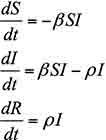
We propose that vaccination moves a member of the cohort from “susceptible” to “removed” at  . (See Figure 1 and Figure 2.) 

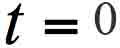
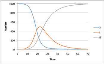
Figure 1: Typical instance of the SIR model, with no vaccination. In this case we have (arbitrarily) chosen At its peak, approximately 50 percent of the population is infected simultaneously, and all members of the population eventually have the disease.

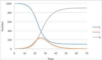
Figure 2: A different instance of the SIR model. This case is the same as shown in Figure 1, except here we have chosen , making the recovery from the disease much faster. The peak is much lower and approximately 10 percent of the population escapes infection with no measures in place. This phenomena was one of Kermack and McKendrick’s initial insights in epidemiology.

Using the model shown in the first equation and Figure 1, we can parametrically vary the percentage of the vaccinated population, who begin at time zero in Class R.

Figure 3 shows the result of our sketch analysis. When the numbers of immune members of the population are high, then the opportunity for spread is lower, and there is a “herd advantage” effect, in that the number of people escaping infection is higher than the vaccinated population. In our sketch, when herd immunity begins to fails, it does so dramatically.

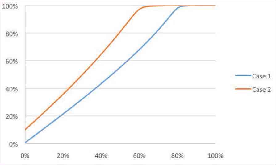
Figure 3: The total amount of the population uninfected in the SIR models shown in Figures 1 and 2. The “uninfected” population is defined as the vaccinated population at time zero (who is immune) as well as the susceptible population at  , who escaped infection. The parameters are arbitrary; the important point from the chart is the phenomena that when herd immunity fails, it fails dramatically.

A note on technique: This analysis was performed in MS Excel, using Euler’s method for integrating the differential equation. The use of data -> what if analysis -> data table automated what would have otherwise been a time-consuming manual process of parametric analysis to produce Figure 3. The data table feature isn’t perfect, and it can be a bit of a “memory hog.” I recommend creating the table and then copy -> paste special -> values.

References

1. Kimberly M. Thompson, Radboud J. Duintjer Tebbens, Mark A. Pallansch, Steven G.F. Wassilak, Stephen L. Cochi, 2015, “Polio Eradicators Use Integrated Analytical Models to Make Better Decisions,” Interfaces, Vol. 45, No. 1, pp. 5-25 (http://dx.doi.org/10.1287/inte.2014.0769).
2. Dimitrov, N. and Meyers, L., 2012, “Mathematical Approaches to Infectious Disease Prevention and Control,” TutORials in Operations Research (http://dx.doi.org/10.1287/inte.2014.0769).
3. https://www.informs.org/ORMS-Today/Public-Articles/June-Volume-41-Number-3/INSIDE-STORY.
4. Daley, D. and Gani, J., 1999, “Epidemic Modeling: An Introduction,” Cambridge University Press.
5. http://www.cdc.gov/measles/multi-state-outbreak.html