

November 7, 2016 in Five-Minute Analyst
The ballot theorem
SHARE: PRINT ARTICLE: https://doi.org/10.1287/LYTX.2016.06.14
This column will appear around the date of the U.S presidential election, and while I have been trying to avoid politics this year, it is simply impossible. I think it is fair to say that this year’s election has been contentious, and millions of people have closely followed the campaign coverage and debates. While in the United States votes are not reported until the election is over, there are “exit polls” on Election Day, which gain insight into the election by asking voters who they voted for as they leave their respective polling locations.
In a closely contested election, it is possible that in any exit poll the eventual loser will lead the eventual winner due to simple random chance. Consider a simple non-election example. In a suite of cards (13 cards), there are nine number cards (2-10) and four non-number cards (Jack, Queen, King, Ace); correspondingly there are 36 number cards and 16 non-numbered cards in a deck. If one were to shuffle the deck, flip the cards over one at a time, and count the numbers as a vote for candidate A and non-numbers as a vote for candidate B, we can see that there are paths where the candidate B would be leading, even though A will be the eventual winner. Specifically, the probability that the first vote will show B having the lead on the first vote is 30 percent. Expanding this approach, counting paths, we can see that there are other paths, beginning with a vote for A, which will have B in the lead, such as 9-K-Q and so on. The way to analyze this is to count paths, and there is an exceptionally elegant solution proposed by Bertrand [1], that the probability that the eventual winner is always ahead is given by:
(p-q)
____
(p+q)
In our example for deck of cards, there is only a 38 percent chance that the “numbers” player will be ahead the entire time.
Application to the 2016 Presidential Election
Depending on the locale, it is either illegal or discouraged to publish exit polls before the polls in that state are closed. This means that voters on the East Coast have no information as to how the voting actually went, but voters on the West Coast (such as myself) will begin getting information about how the nation voted before the polls in their state are closed. Voters may use this information to influence their decision to vote themselves, depending on if they see their candidate as winning by a large margin or losing by a small one.
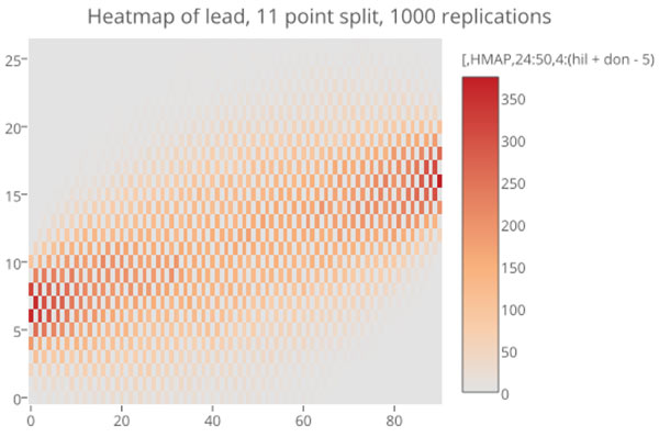
The Washington Post reports that each exit poll location attempts to poll between 100 and 150 persons per location. If for sake of example we take 100 voters in a particular location, and use a current poll estimate, Mrs. Clinton is leading Mr. Trump 55 percent to 44 percent. While computing the probability that Mrs. Clinton leads all day using the formula is trivial, we can use a simulation to consider the traces during the day.
A simulation is useful for seeing this behavior in detail. While there’s a bit more code supporting the analysis, the “business” of the simulation is: Library(magrittr) Votes = c(rep(1,55), rep(-1, 44)) Votes %>% sample() %>% cumsum(). This is one of the (many) advantages of using R Markdown as a =
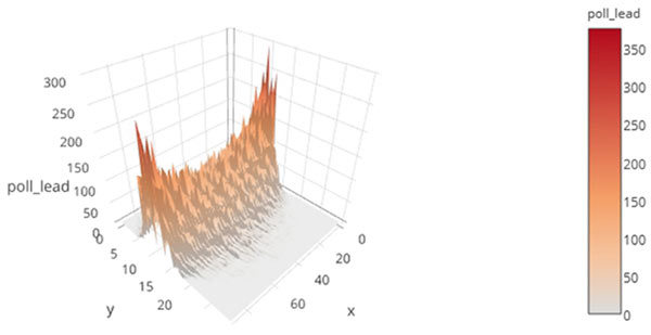
As of mid-October (the time this was written), the polls were changing so rapidly that it was an exercise in futility to try to predict what the polls will be as we approach Election Day. We will overcome this by paramatrizing the possible leads, using the most historic landslide (35 percent) as the benchmark. Note that this is symmetric, so if you like Mr. Trump, the mathematics remain the same.
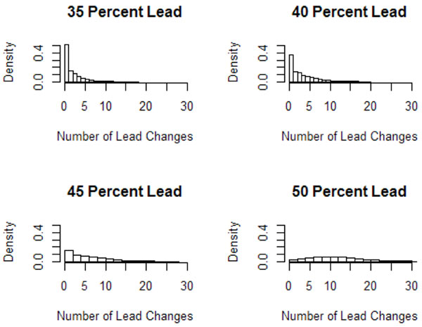
sampled and various lead sizes. As one would expect, the maximum
number of lead changes occur when the race is even.
A few technical issues to close this exploration: I have thought about random walks before in this article, particularly as applied to the Army-Navy football game, which has been the subject of the November column for the past two years. Random walks in the limit become Brownian Motion, first explored in-depth by A. Einstein in 1905. Our example here forms a special type, known as the Brownian Bridge. Unlike our previous examples, which started at a known starting point and moved in either direction towards infinity, the Bridge has a known start and end point. Further discussion is beyond the scope of this article, but is rich in theory and application.
By the time this goes to press, and certainly by the time many of you will read it, the 2016 election will be history.
REFERENCE
- Grimmett and Stirzaker, 2001, “Probability and Random Processes,” Oxford University Press.
Harrison Schramm, CAP, PStat, is a senior lecturer at Naval Postgraduate School, splitting his time between Defense Management and Operations Research where, in addition to teaching, he runs the Contested At-Sea Logistics Lab (CASLL). He served as the inaugural chair of the INFORMS Security Conference and is a past president of the INFORMS Analytics Society.
([email protected])