Rainfall and reference years

This installment comes from a discussion I’ve been having with longtime friend and U.S. Naval Academy classmate Cara Albright. Her problem revolves around determining the “most representative” year of precipitation (rain) data from a large set. The original question – how to incorporate data from years that include “leaps” (i.e., Feb. 29) – started us down an interesting path. This is a fun story about collaboration and thinking about problems.

To make this concrete, consider a graph of two separate year’s raw rainfall data (Figure 1). From this plot, it is unclear what the best method for measuring the “distance” between these two years would be. 

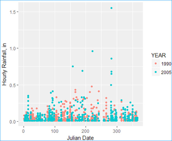
One current approach to this problem is to measure the similarity of the years “pointwise.” Now, those of us who have been alive for a few years (or have seen “The Pirates of Penzance”) know that not every year is the same; most years have 365 days, but a quarter of years have 366. The approaches to dealing with the problematic Feb. 29 are:

1. Ignore it, thus throwing away ~.3 percent of the data.
2. Lump it in with March 1.

Neither of these are particularly satisfactory to us. Instead of trying to measure the distance pointwise – which is highly sensitive to “breakpoints” – hourly and daily, we propose to measure the difference between cumulative precipitation, normalized to 365 days (and thus overcoming the leap year problem).

To measure the difference between years, we follow a simple process of re-normalizing the data to a 365-day “standard year.” We then sum the squared differences between the two years. For those who prefer math over words, we do this:

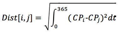
The year with the minimum distance, as determined by the minimum (summed) distance over all other years, is the “reference” year.

Application

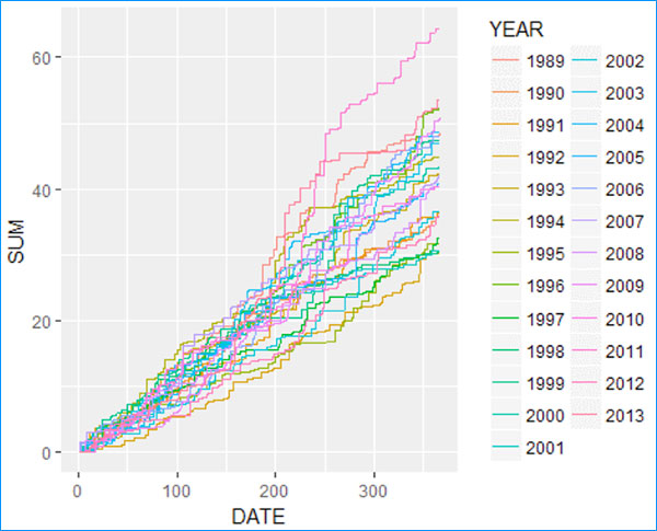
Our current data set consists of 100 years of rainfall data from Philadelphia, as shown in Figure 2. We determine the “representative year” starting in 1965 to the year chosen; in other words, the 1993 point is 1989-1993, 2000 is 1989-2000 and so on. Using this “moving right-hand reference approach,” we see the years chosen as depicted in Figure 3.

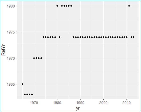
With 1973 chosen as the most frequently representative year, based on minimum distance and a normalized year length. One “might” argue, as we thought, that this approach tends to favor years that have the total rainfall that is closest to average. To overcome this minor difficulty, we may simply normalize the rainfall over the year as well, scaling the total for the year to 1. This “variance only” approach produces the graph shown in Figure 4.

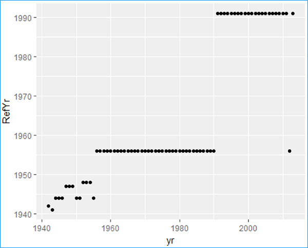
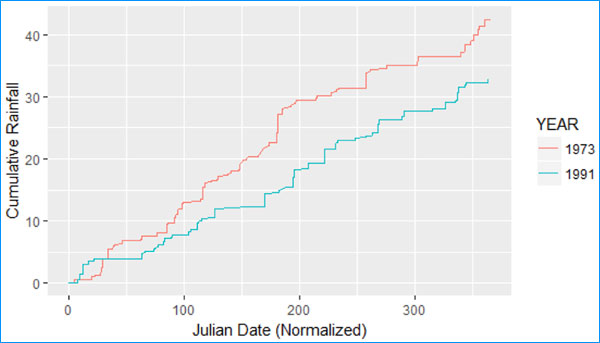
Which tends to favor 1956 and, later, 1991 as representative years. A plot of these two candidates is shown in Figure 5:

In conclusion, we have applied a few more than five minutes worth of analysis this installment. What is more important than the results is that the basic ideas of calculus and statistics, which we don’t always use every day in practice, continue to echo in practice far beyond our basic schooling.

Technical note: This analysis made ample use of the R base function approxfun(), which interpolates between values of a given empirical data set. This made numerical integration quite straightforward.