Public television’s deadliest cities

My daughter plans to study history in college, which is a course of study I fully support. That being said, I expressly forbid her from studying at Oxford for one simple reason – the crime rate is astonishingly high. That’s according to the PBS murder mystery series in which Inspector Morse, and then Inspector Lewis, are confronted with a fresh double- or triple-homicide every week!

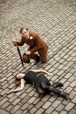
In this episode of the “Five-Minute Analyst,” we survey four of the sleuthing world’s preeminent detectives, culminating in the master himself, Sherlock Holmes, as depicted on PBS shows. Let us introduce the dramatis personae:

Vicar Sidney Chambers has a full-time occupation as an Anglican priest, but for some strange reason he can’t keep away from the police. He helps the overworked Detective Inspector Geordie Keating solve murders – quite a few, in fact, in the town of Grantchester in the mid-1950s. In addition to preaching, solving crimes and pursuing his (married) love interest Amanda, he consumes truly heroic quantities of alcohol while listening to jazz records.

Detective Constable Endeavor Morse (“Young Morse,” later Detective Chief Inspector Morse) works under the watchful eye of Detective Inspector Fred Thursday and makes up for his nonconformist attitude on the police force with a mix of bravery, intuition and alcohol. Despite the constant threat of dismissal from Chief Superintendent Bright, he solves crimes in Oxford in the mid-1960s.

Detective Inspector Robbie Lewis is the overworked and underappreciated junior to DCI Morse, who, by the time of Lewis, is deceased. He carries on the seemingly impossible task of keeping Oxford safe from elaborate and gruesome multiple murders in the early 2010s, with his own Morse-esque assistant, Detective Constable James Hathaway. Lewis likes to take a pint at the public house.

Consulting Detective Sherlock Holmes is not part of any recognized police force. He uses the sheer power of his mind to solve all manner of crime in London to the constant annoyance of his landlady and his assistant – the intrepid Dr. Watson. Holmes does not drink; instead he solves crimes in this updated version of the classic tale, reset in the mid-2010s, to keep him distracted from his intoxicant of choice – heroin.

Now, let’s consider how effective they are at crime-fighting by considering the murder rate in each of their cities. The method is as follows: the number of homicides are determined by reading the synopsis of each episode. Because British TV show seasons are typically a quarter of a year, the per million (how the actual statistic is reported in the U.K.) rate is determined by multiplying the murders in a season by four and dividing by the population (in millions). Population data comes from the U.K. Office for National Statistics. In descending order of murderous behavior:

Sherlock Holmes’ London: With a large and rapidly growing population, Sherlock’s fictional London has an astonishingly low murder rate. With two or three homicides per episode distributed over a population around 8 million, Sherlock’s London is far safer than the United Kingdom as a whole, with an annualized murder rate of 2.5-3.5 per million inhabitants (Figure 1).

Figure 1: Homicide rate in Sherlock’s London (mid-2010s).

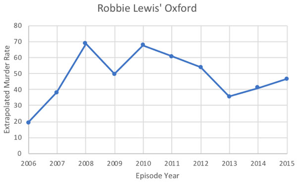
Robbie Lewis’ Oxford: Coming in substantially higher is Oxford, under the watchful eye of DI Lewis. Lewis has a few more homicides per episode than Sherlock, distributed over a smaller population. In any event, DI Lewis is doing slightly better than his mentor (Figure 2).

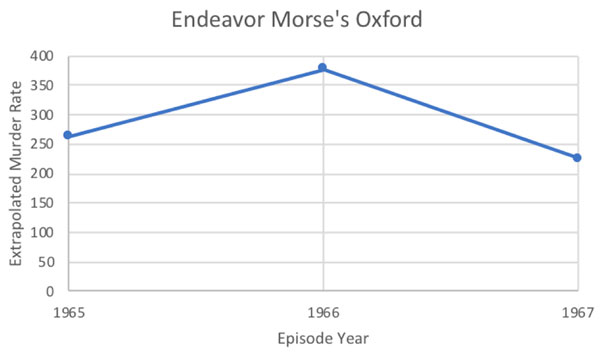
Endeavor Morse’s Oxford (1965): Morse must have learned and passed on quite a bit to his pupil Lewis, as the homicide rate in his Oxford is substantially higher than that of inspector Lewis. This is mostly due to the difference in populations between 2010s Oxford and 1965 (Figure 3).

Sidney Chambers’ Grantchester (1950s): With its quaint country surroundings, comfortable vicarage and lakes for strolling, one would never suspect that Grantchester is the murder capitol of, well, pretty much the universe, with a normalized rate reaching over 51,000 homicides per million! The number of homicides in Grantchester are no greater than those in the other series, but they are distributed over a population of 540.

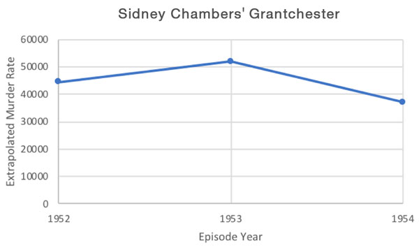
Figure 4: Homicide rate in Sidney Chambers’ Grantchester (1950s).

As an aside, and perhaps to help you sleep better at night, the actual homicide statistics for the United Kingdom are provided in Figure 5.

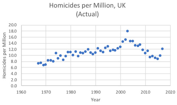
Figure 5: Actual homicides in the United Kingdom (mid-1960s to mid-2010s).

Looking at Figure 5, you might wonder why crime is falling after the year 2000. Several others, including The Economist magazine, have wondered that as well. For more, click here.