

November 12, 2018 in Five-Minute Analyst
World economic growth
How to ‘squeeze’ a bit more knowledge out of a limited data set.
SHARE: PRINT ARTICLE: https://doi.org/10.1287/LYTX.2018.06.14

I am not an economist, but I am interested in the performance of the economy. At work last week, my colleague wanted to know if we could build a model that considered the growth and interaction of some of the world’s biggest economies, based on data from the USDA Economic Research Office. Specifically, he wanted to see if he could extrapolate the data that was in the set out to the future. A plot of the data is shown in Figure 1.
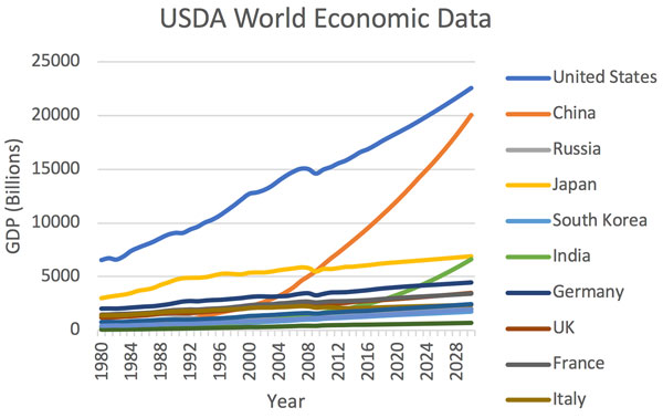
Plot of the USDA World GDP data from the U.S. Department of Agriculture. The data set includes both actual numbers and projections that go to 2030.
Modeling the World Economy
Disclaimer: serious work is done in this area by economists, which I am not!
In order to build a model of this process, I decided to take a differential equation approach and fit the parameters by minimizing the residual deviance. This uses ideas at the crossroads of statistics and optimization, which I have been fascinated by since seeing Dimitris Bertsimas’ Philip McCord Morse Lecture at the 2014 INFORMS Annual Meeting. The development here follows a general class of differential equation models, which have specific use cases in epidemiology (the Kermack-McKendrick SIR model) and modeling combat situations (Lanchester systems). With these ideas in mind, we propose a model of the form:
 ,
,
where X is the vector representing the world economies at time t, and β is the (stationary) matrix of GDP growth. Because the data is presented annually, the natural “scaling” of this model is 1.
Before we discuss the solution methodology, we show the model result in Figure 2.
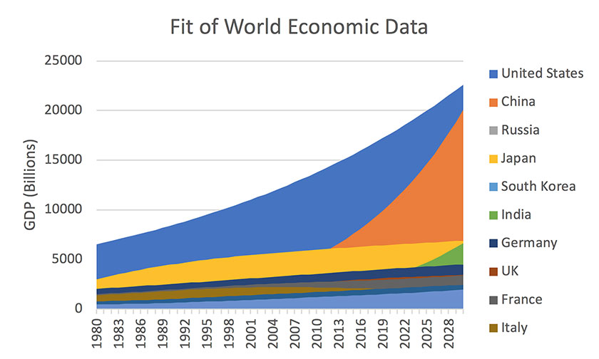
Figure 2: Fit of world economic data using the vector model proposed.
Solution Methodology
As the charts imply, this was done in Microsoft Excel, using the installed Solver. The NLP formulation is:
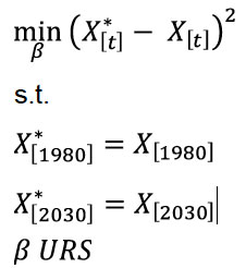
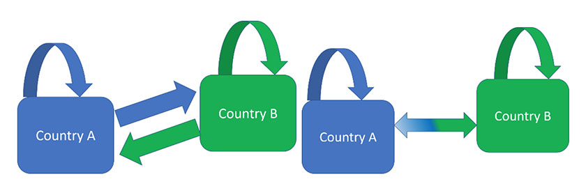
When looking to solve this model, I originally used a full rank matrix with values restricted to be greater than one. My general NLP instinct was that this would work better, as depicted on the left side of Figure 3. However, when it came time to actually solve the optimization problem, the solver worked far better as an “upper triangular” matrix. This is both because of fewer variables in Solver, as well as making the solution more unique.
Assessing Performance
This is a very simple analysis performed with an “adequate” tool using time only as a variable. Because of the way the problem is postulated, we know that the endpoints will “fit” (the problem was posed this way). One way to think about the performance of a model like this is to plot the residuals or “miss” amounts.
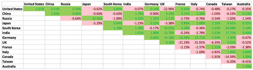
Figure 4: Matrix of growth /decline variables across the economic dataset. The rows are “from” and the columns are “to,” with the interpretation that a nation’s own growth is “to itself” (the on-diagonal elements).
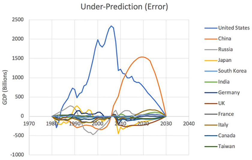
Figure 4: Matrix of growth /decline variables across the economic dataset. The rows are “from” and the columns are “to,” with the interpretation that a nation’s own growth is “to itself” (the on-diagonal elements).
Summary
In summary, this short article shows how to “squeeze” a bit more knowledge out of a limited data set, which is always an implied subtask to any analysis. It was also a fun way to exercise both differential equation models as well as getting MS Excel’s GRG Nonlinear Solver to produce an interesting result.
Harrison Schramm, CAP, PStat, is a senior lecturer at Naval Postgraduate School, splitting his time between Defense Management and Operations Research where, in addition to teaching, he runs the Contested At-Sea Logistics Lab (CASLL). He served as the inaugural chair of the INFORMS Security Conference and is a past president of the INFORMS Analytics Society.
([email protected])