
October 30, 2019 in Five-Minute Analyst
RRt (pronounced ‘Art’)
SHARE: PRINT ARTICLE: https://doi.org/10.1287/LYTX.2019.06.12

I frequently tell my colleagues and friends that working in operations research is very much like traveling by hot air balloon; you know you are going somewhere, but generally, you have no idea where that is when you start. You have to just get aloft and see where the winds – made up of equal parts creativity and data – take you. That’s precisely the story you are going to read today.
It all started years ago when I began graduate school. I had a professor for finite methods who we all thought was “HalF” crazy; he introduced me to ideas about computational complexity based on problems that were intentionally difficult. This is the opposite of what most operations researchers try to do. In the course of studying with him, I was introduced to a truly remarkable volume: “Number Theory in Science and Communication” by Manfred Schroeder [1]. I’m actually on my third copy; previous ones were given away to colleagues who were interested.
Fast forward to the present day. My son is studying prime numbers in 6th grade math class, and, since sieving for prime numbers naturally lends itself to computing, we decided to code up the Sieve of Eratosthenes in (of course) R [2]. Flipping through this section for the first time in several years, I took a peek at two very lovely plots on page 50 of the coprime function of x and y on 2:256, along with its Fourier Transform. As is so often the case, I wanted to make that plot myself [3]. And … we’re off!
First, we mimic the portrait in the book by computing the comprimality of (x,y). To review, two numbers (a, b) are coprime if their only common factor is 1. For example, 4 and 9 are coprime, though neither is prime! There are several ways to compute this; I used the numbers package for R, resulting in a plot that looks like Figure 1.
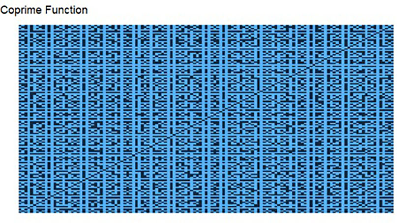
Figure 1: Coprime function.
From here, we can apply a Fast Fourier Transform (FFT). Because the FFT is a complex valued function, you actually have four choices: real, imaginary, modulus and argument (angle). Because this is RRt class, I’ve chosen the one that made the coolest plot as shown in Figure 2.
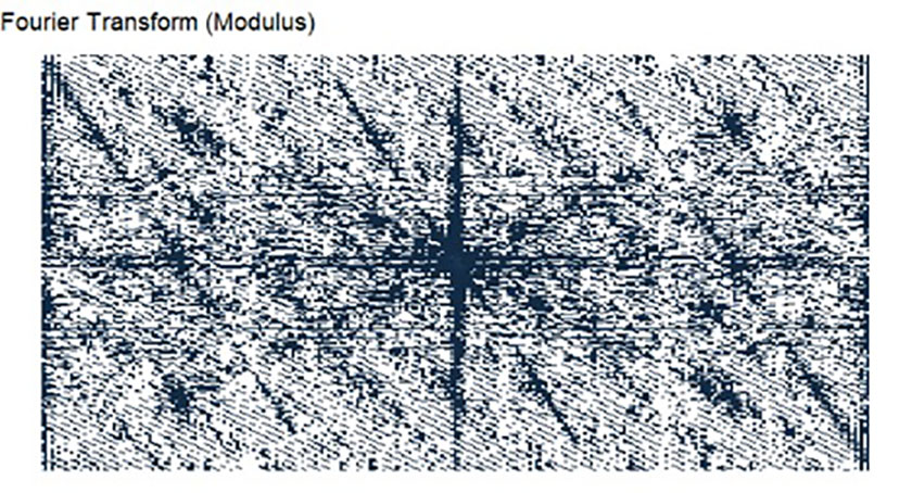
Figure 2: Fourier Transform (modulus).
As a second excursion, we experiment with the greatest common divisor (GCD). This is for some numbers similar to the coprime function; specifically, the GCD of two coprimes is 1. Plotting this from 2:512 results in the somewhat mundane plot shown in Figure 3.
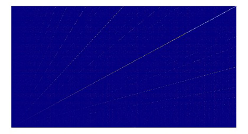
Figure 3: The GCD’s mundane plot.
For our final plot (Figure 4), we show the “argument” or complex angle of the GCD plot. With the correct coloring, we have finally arrived at . . . RRt!
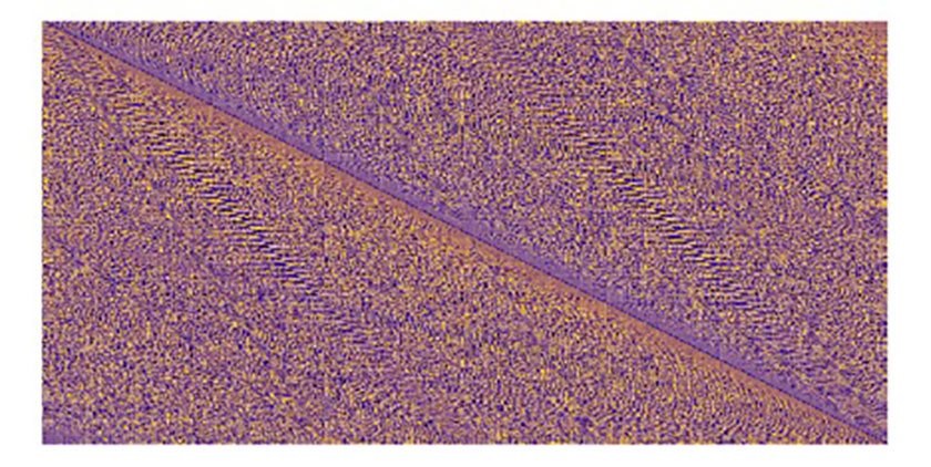
Figure 4: “Argument” of GCD plot results in RRt.
In conclusion, it’s sometimes fun to step away from your projects, and look through other people’s work to see what you think you can do. It’s interesting and fun to see what you can learn along the way.
References and Notes
- https://www.amazon.com/Number-Theory-Science-Communication-Self-Similarity/dp/3540852972
- Not elegant or efficient, but works:
Sieve = function(nmax = 10){
numbers = 2:nmax; Primes = c(); maxSieve = sqrt(nmax)
while(Prime<=maxSieve){
Prime = numbers[1]
Primes = append(Primes, Prime)
numbers = numbers[-which(numbers %% Prime == 0)]
}
Primes = c(Primes, numbers)
} - Do you ever feel that way? If not, you are in the wrong profession.
Harrison Schramm, CAP, PStat, is a senior lecturer at Naval Postgraduate School, splitting his time between Defense Management and Operations Research where, in addition to teaching, he runs the Contested At-Sea Logistics Lab (CASLL). He served as the inaugural chair of the INFORMS Security Conference and is a past president of the INFORMS Analytics Society.
([email protected])