Customer Centricity in Supply Chain Through Optimal Allocation of Supply to Demand and Back Orders – The Power of Prescriptive Analytics

For any customer-centric organization, customer satisfaction is of utmost importance, and the supply chain of the manufacturer needs to operate in a way that ensures consumer satisfaction is one of its key principles. Quality, time and quantity are three dimensions that can ensure customer satisfaction through the supply chain. In the complex array of a supply chain network – comprising suppliers, vendors, manufacturers, distributors and customers – high-quality finished goods from raw materials would ensure quality is maintained and consistent. The third dimension that ensures customer satisfaction is the quantity that can be obtained through an optimal allocation of supply to demand and back orders across multiple customers.

In a business-to-business (B2B) setting, the customer orders materials from manufacturers in bulk, which the ordering customer requires to fulfill the demands on their end. This generates the demand to the manufacturer that they fulfill through the production and supply chain process. The challenge is to accurately estimate or forecast future demands, given the plethora of external factors that need to be accounted for, including unforeseen events. As such, any unmet demands become a back order. As time passes, too many back orders get accumulated if the manufacturer cannot fulfill the back orders along with current demands through its supply. Customers may walk away from old back orders, creating a lost opportunity for the manufacturer.

One strategy to ensure customer satisfaction is meeting the quantity of current demand and back order as best as possible with new supply. When new supply arrives, it must be allocated among different customers so that the difference of actual demand and back orders is minimized. Customer satisfaction would increase as the quantity of demand is met, among other factors. Modern supply chain systems generate lots of data that can be leveraged to develop a data-driven allocation strategy by applying optimization methods and prescriptive analytics. Without a proper allocation system to augment it, once the supply arrives at distribution centers, the quantity factor of customer demand would not be satisfactorily met.

Model Description

A supply chain for any manufacturer starts with raw materials required for production, manufacturing hubs for producing finished goods, and different levels of distribution centers through which it distributes its products to its customers. For a simplified model, the demands from the customers come to the distribution center, and the supply from the manufacturer is distributed to its customers through its distribution center. When new supply arrives for a particular product, the challenge is whether to allocate the new supply to current demand or existing back orders, and in what proportion the current supply can be allocated to different customers of varying demand sizes and customer prioritization. As mentioned in the problem statement, one important outcome of the allocation is ensuring customer satisfaction in meeting the quantities that have been asked for in demand and existing back orders.

The overall flow is a closed-loop feedback-based system in which the manufactured product reaches the distribution center. This is the total current supply, which is divided in proportion to overall back order and current demand or any other predetermined ratio for allocation. To avoid lost opportunity, the distribution center may start with the back order nearest to the cutoff time for allocation. Cutoff time is the time beyond which any unmet back order becomes a lost opportunity because the customer may not proceed with the order. The proportions for the overall back order and current demand are then allocated to individual customers in proportion to their actual back orders and individual demands, along with considering any customer-specific prioritization. (The mathematical formulation for the allocation model is detailed later.) Once the allocation has been calculated for each customer based on the mathematical formulation, a validation check is performed to ensure the current supply is fully allocated. As a closed-loop feedback-based system, the allocation model continues to track the actual demand and back orders with the allocation based on the formulation every time a new supply comes. This enables monitoring the performance of the allocation model with time as well as identifying any changes in actual demand and back orders. A well-operated supply chain system with systematic allocation may show a decrease in the back order quantities with time. This allocation model is also applicable to different levels of the distribution center, whether central, regional or local.

Mathematical Formulation

Raw materials go through different stages of manufacturing to produce finished goods, which travel through different modes of transport and through regional and local distribution centers. The supply quantity of finished goods is based on estimates from demand. Accurately forecasting demand for a global supply chain network is nontrivial because it is based on historical data, and a plethora of dynamic events are regularly occurring for which there are often gaps that arise between demand and supply. Two types of situations arise, including:

1. The incoming supply is greater than the current actual demand.
2. The incoming supply is less than the current actual demand.

However, Situation 2 is more prevalent when the current supply is less than the current actual demand, and the current demand that could not be fulfilled with the current supply leads to back order. The mathematical formulation is based on Situation 2.

Solve for: Weights of customers,

Objective function: Minimize the difference between actual back order and allocated to back order, and actual current demand and allocated to current demand

Minimize

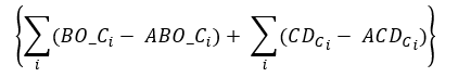
∀ i = 1, 2, 3, ... n 

Constraints:

BO_C_i = Actual back order of customer i

ABO_C_i = Allocation to fulfill back order for customer i

CD_C_i = Actual current demand of customer i

ACD_C_i = Allocation to fulfill current demand for customer i

1. 

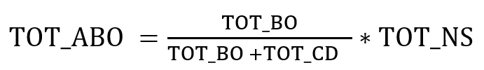
Current total supply is allocated to the total back order in proportion to the total actual back order and actual current demand.

TOT_ABO = Total allocated to back order

TOT_BO = Total actual back order to all customers for the particular material

TOT_CD = Total actual current demand of all customers for the particular material

TOT_NS = Total current supply of the particular material

2. TOT_ACD = TOT_NS − TOT_ABO

The residual from proportional allocation of current supply to total back order is allocated to meet current demand.

TOT_ACD = Total allocated to demand fulfillment

3. 

Individual customer back order is allocated in proportion to its actual individual back order.

4. 

Individual customer demand fulfillment is allocated in proportion to its actual individual back order.

5. w₁ > w₂ > ... > w_n 

Weights to account

6. 1 < w_i < 10              ∀ i = 1, 2, 3, ... n 

Range for weights

7. BO_C_i − ABO_C_i > 0                ∀ i = 1, 2, 3, ... n 

To avoid absolute objective function

8. CD_C_i  − ACD_C_i > 0              ∀ i = 1, 2, 3, ... n 

To avoid absolute objective function

Validation: Validation ensures that the current supply is allocated to the maximum to fulfill the current demand and back order(s).

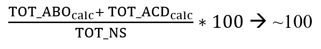
TOT_ABC_calc = Total allocated to back order, after calculated allocation to each customer

TOT_ACD_calc = Total allocated to demand fulfillment, after calculated allocation to each customer

Scenarios

• S: Total current supply
• D: Total current demand
• BO₁, BO₂, BO_3: Back orders at time periods 1, 2, 3 (higher number, further in time)
• BO₃: Back order at cutoff time period (beyond this, all back orders become lost opportunity)

Furthest first scenarios work in situations where the current supply allocation starts with the furthest back order (in time scale, which has not become write-off yet), in addition to allocation to current demand. Different scenarios that can be met by variations of allocation formulation are as follows:

• Scenario 1: S > BO₃, D; S ≤ BO₂ + D
• Scenario 2: S < BO₃ | D
• Scenario 3: (Spillover allocation) S > BO₃, D; S > BO₃, +D; S ≤ BO₃ + BO₂ + D
• Scenario 4: Spillover to more recent back order time periods
• Scenario ideal: S ≥ BO₃ + BO₂ + BO₁ + … + D

Nearest first scenarios work in situations where the current supply allocation starts with the nearest back order (in time scale) in addition to allocation to current demand. Different scenarios that can be met by variations of allocation formulation are as follows:

• Scenario 1: S > BO₁, D; S ≤ BO₂ + D
• Scenario 2: S < BO₁ | D
• Scenario 3: (Spillover allocation) S > BO₁, D; S > BO₁, +D; S ≤ BO₁ + BO₂ + D
• Scenario 4: Spillover to more recent back order time periods
• Scenario ideal: S ≥ BO₃ + BO₂ + BO₁ + … + D