January 7, 2026 in Optmization
From Optimization Models to Policies: The Power of Parameterized Deterministic Optimization Models
SHARE: PRINT ARTICLE: https://doi.org/10.1287/LYTX.2026.01.01

If you work in operations research (O.R.), you have seen the following countless times: Someone creates an optimization model (using a mixed-integer linear programming model (MILP)) to solve some business problem:
minx,y C(x,y) (1)
subject to
G(x,y) = 0, (2)
x ≥ 0, (3)
y ∈ (0,1). (4)
With the advent of powerful solvers (mostly after the year 2000) that could handle a wide range of integer programming problems, we now have the tools that can handle many practical applications. This means that we can raise our hands and exclaim, “It is optimal!”
Boy, we do love that word “optimal.” George Dantzig popularized the idea of designing an algorithm (initially the simplex algorithm) to solve a problem and then proving that the solution is optimal.
Dantzig’s original work in optimization was motivated by the challenge of improving operations in the military. One problem that he encountered involved the assignment of “resources” (pilots, aircraft) to “tasks” (flights, targets). If you have 10 resources and 10 tasks, you have 10! = 3,628,800 possible solutions. His simplex algorithm could solve problems like this (and today, problems that are far larger). Assignment problems are actually quite easy because they exhibit very special structure; the solvers today can handle problems that are much more difficult, such as scheduling a fleet of power generators for the grid.

From Static to Sequential Problems
There is just one problem: We never solve these operational problems just once – we are always solving them repeatedly over time. Most often (but not always), the solution of a problem at one point in time affects problems in the future.
This means that our Problem (1)–(4) should be indexed by time t, where all the data is captured by a variable we will call St (the “state variable”). In this case, our MILP might be written as:
minxt,yt Ct(xt,yt | St) (5)
subject to
Gt(xt,yt | St) = 0, (6)
xt ≥ 0, (7)
yt ∈ (0,1). (8)
where we write Ct(xt,yt | St) and Gt(xt,yt | St) to express the dependence of these functions on information in St.
Practitioners of the craft of optimization realize this and often introduce ad hoc adjustments to the model to handle the downstream impact of solutions now on the future. In fact, they also realize that random events mean the solution (xt,yt) in the model is not always implemented exactly in the field.
These changes require choices in terms of how the objective function and constraints are modified, and the introduction of tunable parameters. We are going to let f represent the choice of modifications (in effect, the functions) and θ be any tunable parameters. For reasons we will reveal momentarily, we are going to let π = (f,θ) be the combination of function f ∈ F and parameters θ ∈ Θf, and we will denote the modified objective function and constraints by Cπ(xt,yt | St,θ) and Gπ(xt,yt | St,θ).
Finally, we are going to recognize that we are not so interested in the optimal value of Cπ(xt,yt | St,θ). Rather, we are interested in our decisions (xt,yt) and how well they work over time. We are going to designate the single function Xπ(St | θ) as the optimal solution to the problem in (5)–(8), which we can write as
Xπ(St | θ) = arg maxxt,yt Cπ(xt,yt | St,θ) (9)
subject to (6)–(8). The function Xπ(St | θ) defined by (9) along with (6)–(8) is called a policy, or “a method for making a decision.”
The term “policy” is widely used in the field of Markov decision processes, in which it is almost always a rule such as “buy low, sell high” or “when the inventory is less than s order up to S.” However, we can view a policy as any function that returns a decision given the information in the state variable St, including functions that require solving large-scale integer programs.
The way we evaluate the policy is to sum our performance metric (assuming there is one) using
Fπ(θ,S0) = ∑t=0T C(Xπ(St | θ) | St), (10)
where we assume that our "state variable" St evolves according to set of equations known as the transition function, which we write as
St+1 = SM(St, xt = Xπ(St | θ), Wt+1). (11)
The variable Wt+1 introduces any information that we first learn about after we make the decisions (xt,yt) at time t and before we make the next decision (xt+1,yt+1); Wt+1 might capture demands for products, travel times, costs, and prices.
Because we do not know Wt+1 when we determine (xt,yt), these decisions have to be determined given the uncertainty of this information. Technically, we should insert an expectation in front of the summation in (10), but we often evaluate a policy by simulating over a single sample path (a topic for another conversation).
The objective function that any company is interested in is given by Fπ(θ,S0) in Equation (10). In addition, we are not optimizing over (xt,yt). Rather, we are interested in optimizing over our policies π = (f,θ). We then write our optimization problem as
minπ=(f,θ) Fπ(θ | S0) = minf minθ ∈ Θf ∑t=0T C(Xπ(St | θ) | St). (12)
We have now written (12) as a nested optimization problem, where we first optimize over functions f ∈ F and then optimize over the parameters θ ∈ Θf. In practice, the search over functions f is fairly ad hoc – it involves people combining intuition about the problem with an understanding of how to affect the behavior of the optimization problem embedded in Xπ(St | θ).
The optimization problem in (12) represents two very different optimization challenges that need to be addressed by two different communities:
- The design and evaluation of functions f ∈ F need to be handled by domain experts. This requires an understanding of how uncertainty might affect the solution that will guide how the optimization model is parameterized.
- Tuning of the parameters θ requires access to a simulator. With a simulator, this becomes a straightforward (albeit difficult) stochastic optimization problem. However, there will be complex problems in which domain expertise is needed as well.
An Energy Application
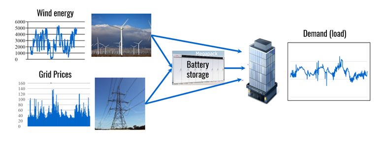
I first came to appreciate this approach to handling uncertainty in a complex optimization problem by watching how grid operators plan schedules for power generation tomorrow to ensure that the grid will not suffer any blackouts if the biggest generators fail. I can illustrate this strategy in the context of a much simpler energy storage problem, shown in Figure 2. Here, we have to pull energy from either a wind farm, where the energy is free but very volatile, or the grid, where we can assume an unlimited supply but at highly stochastic prices. We have to meet the needs of a reasonably predictable demand, assisted by access to an energy storage device.
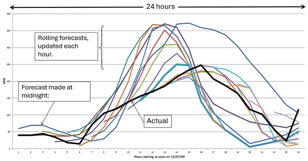
We have access to rolling forecasts of the energy that will be created by the wind farm, as given in Figure 3. We need these forecasts because we have to work with tight capacity constraints for storing the energy. However, the forecasts are updated hourly; these are represented in our state variable St, and the updates arrive through the variable Wt+1. These forecasts are clearly not very accurate, so this represents an important source of uncertainty.
Given the need to plan into the future, the most natural approach was to use a classical rolling horizon procedure that requires solving a linear program that captures flows for 24 hours into the future, shown in Figure 4. However, this means using the forecast of energy from wind as if it were perfectly accurate. Instead, we chose to insert a coefficient θτ for a forecast of wind energy τ hours into the future.
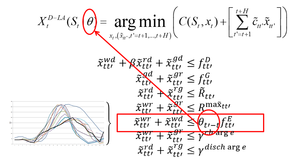
The decision to insert this coefficient in front of the forecast is an example of our parameterization f. We could have chosen to insert coefficients in front of other variables, but our intuition was that this is a main source of uncertainty. We could also have inserted additive adjustment terms. All of these represent different parameterizations f.
It goes without saying that we obtain an optimal solution to the linear program at each time step. Yes, the solution is optimal! But it is not an optimal policy.
Each of these parameterizations includes tunable parameters θ. We next have to optimize Fπ (θ│S0) (Equation (12)) using some algorithm. We used Spall’s SPSA (Simultaneous Perturbation Stochastic Approximation) algorithm [1] – a form of derivative-based stochastic search – which requires computing numerical derivatives using a simulator. This is not easy. Simulating the policy is very noisy, so we would perform repeated simulations (known as “mini-batches” in the stochastic search literature). Figure 5 shows experiments for different values of the mini-batch parameter [2].
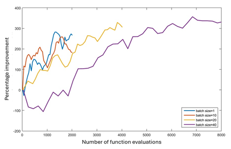
Figure 5. Improvement in simulations of the policy as we tune the policy.
The real point of showing Figure 5 is to demonstrate the improved performance of the policy. Remember that each point on these graphs is the result of solving our linear program “to optimality!” at each point in time in the simulation. Although we always obtain optimal solutions, we are changing the model to produce better results over time
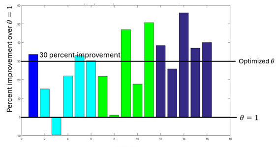
How well does this work? Figure 6 shows the results of a series of runs to optimize θ, where we compare the performance to what we would get by using θ = 1. We note that θ = 1 would, in fact, be optimal if the forecasts were perfect. For the actual forecasts under real-world conditions, we obtain on average of 30% improvement over using θ = 1. addition, the policy is still just a deterministic linear program no larger or more complex than a vanilla lookahead policy with θ = 1!
A challenge anyone has to face when tuning is how to evaluate a policy. This requires:
- Generating samples of the information process W1, W2, ..., Wt ...
- Running a simulation using the parameterized policy along with the information process.
There are three strategies we might try:
- Use historical observations of the information process and then test the policy in an offline simulator (that has to be built).
- Generate samples of the information process from a mathematical model that the behavior of the random information.
- Use trial and error in the field rather than a simulation model.
All three are valid alternatives depending on the situation. Option 1 is widely used in finance, where historical price processes are easy to observe.
Option 2 is needed when we do not have historical data, which is typical when the random information process depends on the decisions being made. A simple example of this arises in inventory modeling, where we observe sales but not the raw market demand. Sales are subject to stockouts, which depend on our inventory decisions.
Option 3 is required when we simply cannot simulate a process, such as market behavior. For example, we can never use a simulator to optimize the price of a product. More often, companies fall back to Option 3 because they do not have the resources to build accurate simulators. This is the approach used by the grid operator that motivated the work in our energy application. They set their parameters θt on day t and then observe the performance on day t + 1, after which they make ad hoc adjustments.
Online tuning is hard, but it is by far the most widely used in practice. The problem is that the tuning process is completely ad hoc, and neither companies nor the academic research community recognize that this process needs to be refined rather than replaced. Online is an overlooked research challenge!
References
- Powell, W.B., 2022, “Reinforcement Learning and Stochastic Optimization: A Unified Framework for Sequential Decisions,” Hoboken, N.J.: John Wiley and Sons.
- Ghadimi, S. and W.B. Powell, 2024, “Stochastic Search for a Parametric Cost Function Approximation: Energy Storage with Rolling Forecasts,” European Journal of Operational Research, Vol. 312, No. 2, pp. 641-652.
Warren B. Powell is professor emeritus, Princeton University, and chief analytics officer, Optimal Dynamics.