Coronavirus and Analytics: Flattening the Curve

“When there’s a war, study the War” – Professor Wayne Hughes 

Note: As this piece was going to press, celebrities such as Tom Hanks [1] reportedly contracted coronavirus (COVID-19), the United States announced a travel ban from many European countries [2], and the World Health Organization declared the disease a pandemic given its worldwide spread. The CDC’s numbers cited below are as of March 11. 

I, like many of us, have had my attention turned in recent weeks to the coronavirus (COVID-19) and associated controls around it. It seems to dominate the news cycle and also people’s actions, with shelves bare of soap and hand sanitizer. This is combined with a mandated silence [3] from government health officials (i.e., real epidemiologists). In their absence, we can consider a few high-level thoughts about analytics and coronavirus.

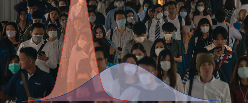
If you are worried about coronavirus – good; you should be. Having said this, small things are likely to have a big impact, and the measures that are being put in place – reducing congregation and increasing hygiene – are likely to have a large impact in the control of the disease. A phrase that has gotten a lot of attention in both social and “real” media is “flattening the curve.” We’re going to spend the remainder of this piece focused on that.

Epidemics, their study and control have a rich history. I’ve been interested in epidemics and their models for a long time now as proxies for computer viruses as demonstrated in serious journals [4], as well as some light-hearted examples involving zombies [5]. For someone who wants to learn about this topic, I recommend the excellent, although highly technical, “Epidemic Modeling: An Introduction” by Daley and Gani (Cambridge U. Press, 1999), as well as Chapter 17 of “Networks: An Introduction” by M.E.J. Newman (Oxford U. Press, 2010).

“Flattening the curve” can be achieved with simple measures (such as handwashing) and when done in aggregate can have a big impact on the spread of disease. The remainder of this article is written at an executive level; the technical appendix may be accessed here. 

Mechanics

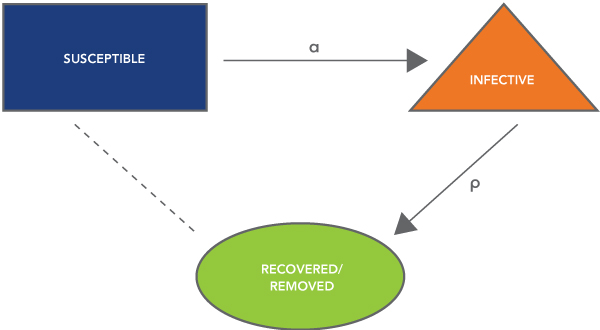
For our development, we will use the Kermack-McKendrick epidemic model, which considers how individuals in a population move from “susceptible” to “infective” and finally to “removed.” The definitions are straightforward but repeated here for completeness:

• Susceptible individuals do not have the virus and may become infected.
• Infected individuals have the virus and may spread it to others until they no longer have the infection and become members of the removed class.
• Removed individuals have run the course of infection and are no longer infected or susceptible to infection.

A graph showing the relationship between the classes is presented as Figure 1.

Flattening the Curve: Theory

We admit immediately that we are using deterministic, aggregate measures to make an inference on an infection process that has small numbers, where stochastic effects are important. We proceed this way for two reasons: first, because the granularity of the modeling approach matches the data that we had available; and second, because these models are simple and serve to illustrate the point.

The model shown in Figure 1 has two unknown parameters. The spread rate, which is an aggregation of several factors, includes:

• the virulence of the disease, which is a factor of the pathogen itself;
• the probabilistic odds of exposure given opportunity, which is a factor of how likely one is to be exposed to the pathogen given that they are in contact with an infected individual; and
• mixing, by which we mean the intensity at which individuals in a population interact with each other.

A typical time trace of an SIR epidemic is shown in Figure 2. 

Fitting Data

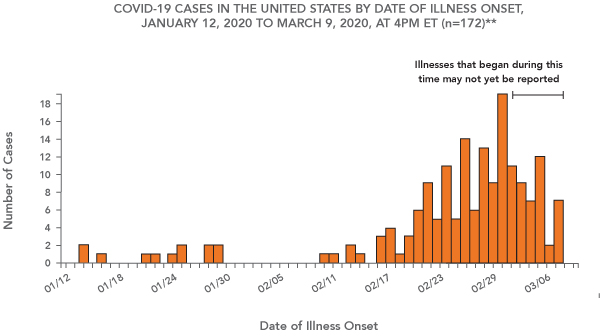
Data about the coronavirus is methodologically wrought with problems. This is partially due to governmental responses to the epidemic, but in our opinion, it is also because the epidemic is ongoing. Data for the outbreak in the United States as reported by the Centers for Disease Control and Prevention (CDC) is shown in Figure 3 [6].

The data is also available in raw format, which we have pulled from the website and produced a plot of cumulative new cases in the United States (Figure 4).

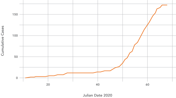
We have made estimates of the two parameters, alpha and rho, based on data, which are listed in the technical appendix. Note that because it is still early in the epidemic trajectory in the United States, we have little confidence in parameter estimates; they are used as a tool for exposition. 

Flattening the Curve in Practice

Mathematically, the control of epidemics rests in two strategies: decrease the infectivity parameter, alpha, or increase the speed of recovery, rho. Revisiting our description from above, we can frame the actions as follows:

• Decrease the probabilistic odds of exposure given opportunity by increasing sanitation measures, such as masks, hand washing, hand sanitizing.
• Decrease the opportunity for exposure by reducing the intensity with which people interact, limiting travel, encouraging people to stay home/work from home and reduce large public events.
• Increase the speed at which people recover, indirectly, by quarantining infected individuals to include self-quarantine.

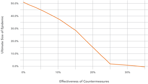
Using our presumptions about the intensity of spread to estimate the infectivity parameter, we can consider how the effectiveness of prophylactic measures taken in aggregate as listed above can impact the trajectory of the infection curve:

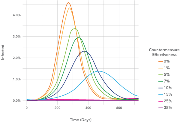
Decreasing the rate of infection both slows the number of cases at any given time (as seen by the flattened curves), but also tends to limit the ultimate distribution of the epidemic itself.

Conclusion: Wash Your Hands

After spending a few days with these models, I am convinced that the measures being put in place – increased focus on handwashing, reducing nonessential travel and encouraging people to stay home whether symptomatic or not – are worthwhile. Of note, general germ hygiene to include handwashing is likely a low-cost, high leverage measure.

This has been a very quick look at a serious problem. Admittedly, there are far more nuanced techniques that could be brought to bear. In the future, it will be interesting to know how effective the measures taken against coronavirus were against infectious diseases writ large – to include the common cold, upper respiratory infections and influenza.

What we are not able to answer at this time is: When will we be able to resume “normality”? This will depend in large measure on our understanding of the disease transmission as it develops in the coming days and weeks.

References

1. https://www.nytimes.com/2020/03/12/world/australia/tom-hanks-rita-wilson-coronavirus.html
2. https://www.cdc.gov/coronavirus/2019-ncov/travelers/index.html
3. https://www.nytimes.com/2020/02/27/us/politics/us-coronavirus-pence.html
4. Schramm, H. C. & Dimitrov, N. B., 2014, “Differential equation models for sharp threshold dynamics,” Mathematical Biosciences, Vol. 247, No. 1, pp. 27-37, https://doi.org/10.1016/j.mbs.2013.10.009.
5. https://pubsonline.informs.org/do/10.1287/LYTX.2013.05.14/full/
6. https://www.cdc.gov/coronavirus/2019-ncov/cases-in-us.html, retrieved March 11, 2020.