
March 2, 2026 in Forum
What Is Learning? The Two Sides of Linear Regression
SHARE: PRINT ARTICLE: https://doi.org/10.1287/orms.2026.01.09
As firms work to move artificial intelligence (AI) into effective decision support [1] for managing demand supply networks, the hot topic is, “What is learning?” The purpose of this article is to generate discussion on this topic and provide my two cents.
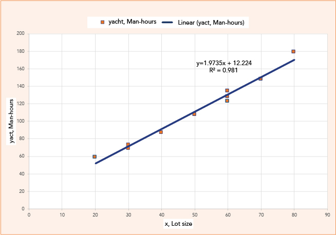
The linear statistical model, aka linear regression (LR) or “best fit” straight line, is a well-known statistical modeling method and a foundational method in machine learning (ML). The core of LR is to find the straight line that best fits the data points collected. Our example is lot size versus man-hours, where we want to predict man-hours based on lot size. This data is provided in Table 1 (columns 1-3) and Figure 1.
| id |
x, Lot size |
yact, Man-hours |
X(i) - XAVE |
(X(i)-XAVE)^2 |
K(i) - weights |
| 001 |
30 |
73 |
-20.00 |
400.00 |
-0.0059 |
| 002 |
20 |
59 |
-30.00 |
900.00 |
-0.0088 |
| 003 |
60 |
128 |
10.00 |
100.00 |
0.0029 |
| 004 |
80 |
179 |
30.00 |
900.00 |
0.0088 |
| 005 |
40 |
87 |
-10.00 |
100.00 |
-0.0029 |
| 006 |
50 |
108 |
0.00 |
0.00 |
0.0000 |
| 007 |
60 |
135 |
10.00 |
100.00 |
0.0029 |
| 008 |
30 |
69 |
-20.00 |
400.00 |
-0.0059 |
| 009 |
70 |
148 |
20.00 |
400.00 |
0.0059 |
| 010 |
60 |
123 |
10.00 |
100.00 |
0.0029 |
| ave |
50.00 |
110.90 |
|
|
|
| sum |
|
|
|
3400.00 |
0.0000 |
| b1 |
1.9735 |
|
|
|
|
| b0 |
12.2235 |
|
|
|
|
Table 1: Lot size vs. man-hours for linear regression demonstrating weighted average solution from the "before times."
A primer on linear regression can be found in the 2024 Q1 article in the International Journal of Applied Forecasting [2]. We want to find values for β1 and β0 (coefficients) such that the estimated man-hours best match the actuals, where estimated hours = β0 + β1 × lot size. The “best” values are called b0 and b1. “Best” is defined as minimizing the difference between the actual value and predicted value.
Within the ML community, LR is often the starting point for supervised or error-based learning. Chapter 7 of “Fundamentals of Machine Learning for Predictive Data Analytics” [3] provides a detailed description of LR from an ML perspective. ML relies on a method called gradient descent [4] that iteratively [5] “learns” its way to the best values for β0 and β1. This sounds exciting and clearly is learning.
But maybe there is an inconvenient fact – LR was invented in the early 1800s [6] and has been a staple of statistical modeling for more than 100 years. So how did they find to the best values for β0 and β1 in the “before times?” To answer this question, we go to Chapter 7 in the classic text “Applied Linear Statistical Models” [7]. It turns out that, when using partial derivatives and simultaneous equations, there is a simple formula in which b1 is a weighted average (see Table 1, column 6) of the Y (man-hours).
The variables and equations are:
- X(i) are the lot size values, where I = 1-10.
- XAVE is the average value for X, which is 50.
- Y(i) are the actual man-hours, where I = 1-10.
- YAVE is the average for Y, which is 110.90.
- K(i) are the weights.
- b1 is the value of β1 that is the best match.
- b0 is the value of β0 that is the best match.
![]()
![]()
![]()
Columns 4-6 in Table 1 show the calculations. With this approach, finding b0 and b1 (best values for β0 and β1) looks more like an algorithm than learning. The “best” β0 and β1 values are 12.2235 and 1.9735, respectively.
What if there are multiple X variables? For example, we add weight and material type to lot size. This is multiple linear regression, and there are standard “matrix or linear algebra” formulas [7] to find the best coefficients. Additionally, linear least squares primitives have been available in programming environments [8] since the early 1970s.
To add to the “mystery”:
- If β0 and β1 have the respective values of 0 and 2.185, the fit is almost as good. A slight change in the slope (β1) enables a large change in the y intercept (β0).
- The values b0 and b1 can be found using the optimization method linear programming that supports a diversity of constraints [9].
Ongoing Challenge
Is linear regression “learning,” statistical modeling or optimization with linear programming? Does it matter for a company which one it is? Let’s discuss learning and how AI can help drive smarter decisions to improve organizational performance – the ongoing challenge.
References
- Fordyce, K., 2023, “A Brief Historical Perspective on Integrating New Decision Support Technology into the Supply Chain Management Decision Process,” OR/MS Today, May 1, https://doi.org/10.1287/orms.2023.02.07.
- Fordyce, K., 2024, “Linear Regression with a Time Series View, Part 1: Simple Linear Regression,” Foresight: International Journal of Applied Forecasting, Vol. 72, No. Q1, pp. 35-39.
- J. D., Mac Namee, B. and D’Arcy, A., 2015, Fundamentals of Machine Learning for Predictive Analytics: Algorithms, Worked Examples, and Case Studies, 2nd ed., Cambridge, MA: MIT Press.
- Fordyce, K., 2025, “Tutorial Gradient Search (Machine Learning Work Horse) from Children’s Slides to Partial Derivatives,” Working paper, Available from author, [email protected].
- Fordyce, K., 2015, “Generate, Test, Next: Computational Principles That Support Import Decision Technologies,” Arkieva, July 7, https://blog.arkieva.com/generate-test-next/.
- Stanton, J. M., 2001, “Galton, Pearson, and the Peas: A Brief History of Linear Regression for Statistics Instructors,” Journal of Statistics Education, Vol. 9, No. 3, https://doi.org/10.1080/10691898.2001.11910537.
- Neter, J., Wasserman, W. and Kutner, M. H., 1974, Applied Linear Statistical Models, Homewood, IL: Richard D. Irwin Inc.
- Polivka, R. and Pankin, S., 1975, APL: The Language and Its Usage, Hoboken, NJ: Prentice-Hall.
- Fordyce, K. and Tenga, R., 2025, “Linear Programming a Better Solution Method for Linear Regression,” Working paper, Available from author, [email protected].
Ken Fordyce is the director of analytics without borders at Arkieva. He joined Arkieva in 2013 after completing a 36-year career with IBM covering a wide range of analytics applications from supply chain to colon cancer. Ken was lucky enough to be part of teams that altered the landscape of best practices in central planning, dispatch scheduling, artificial intelligence, applied optimization and data science. These teams received major awards from IBM, IBM customers, INFORMS, AAAI and POMS.