


Mutual Information Surprise: Rethinking Unexpectedness in Autonomous Systems
Abstract
A community of researchers appears to think that a machine can be surprised and have introduced various surprise measures, principally the Shannon surprise and the Bayesian surprise. The questions of what constitutes a surprise and how to react to one still elicit debates. In this work, we introduce mutual information surprise (MIS), a new framework that redefines surprise not as an anomaly measure, but as a signal of epistemic growth. Furthermore, we develop a statistical test sequence that could trigger a surprise reaction and propose a MIS-based reaction policy that dynamically governs system behavior through sampling adjustment and process forking. Empirical evaluations—on both synthetic domains and a dynamic pollution map estimation task—show that a system governed by the MIS-based reaction policy significantly outperforms those under classical surprise-based approaches in stability, responsiveness, and predictive accuracy. The important implication of our new proposal is that MIS quantifies the impact of new observations on mutual information, shifts surprise from reactive to reflective, enables reflection on learning progression, and thus offers a path toward self-aware and adaptive autonomous systems. We expect the new surprise measure to play a critical role in further advancing autonomous systems on their ability to learn and adapt in a complex and dynamic environment.
History: Kwok Tsui served as the senior editor for this article.
Funding: This work was supported in part by the National Science Foundation [Grant CNS-2328395].
Supplemental Material: The online appendix is available at https://doi.org/10.1287/ijds.2026.0182.
1. Introduction
In July 2020, Nature published a cover story (Burger et al. 2020) about an autonomous robotic chemist—locked in a laboratory for a week with no external communication—independently conducting experiments to search for improved photocatalysts for hydrogen production from water. In the years that followed, Nature featured three more articles (Merchant et al. 2023, Szymanski et al. 2023, Dai et al. 2024) highlighting the transformative role of autonomous systems in materials discovery, experimentation, and even manufacturing, each reporting orders-of-magnitude improvements in efficiency. These reports spotlighted the intensifying global race to advance autonomous technologies beyond the already well-established domain of self-driving cars (Levinson et al. 2011, MacLeod et al. 2020, Yurtsever et al. 2020, Bogdoll et al. 2022). Nature was not alone; numerous other outlets have documented the surge in autonomous research and innovation (Park and Tran 2012, Reis et al. 2021, Leng et al. 2023). This rapid expansion is a natural consequence of recent advances in robotics and artificial intelligence, which continue to push the boundaries of what autonomous systems can accomplish.
The systems featured in the Nature publications demonstrate highly capable bodies that can perform complex tasks. Recall that an autonomous system comprises two fundamental components: a brain and a body—colloquial terms for its control mechanism and its sensing-action capabilities, respectively. Unlike traditional automation systems, which follow predefined instructions to execute simple, repetitive tasks, true autonomy requires a higher level of cognitive capacity—an autonomous system is supposedly capable of making decisions with minimal human intervention. However, the brain function of the current systems, although more sophisticated than rigid preprogrammed instructions, remains relatively limited.
Surveying the literature over the past decade, we found that Nikolaev et al. (2016), Chang et al. (2020), and Burger et al. (2020) rely on classical Bayesian optimization to guide system decisions—a technique that, although effective, does not constitute full autonomy, that is, eliminating human involvement. More recent works in Nature (Merchant et al. 2023, Szymanski et al. 2023) continue in a similar vein, adopting active learning frameworks akin to Bayesian optimization, without fundamentally enhancing the cognitive capabilities of these systems. The conceptual limitations of their decision-making mechanisms continue to impede progress toward genuine autonomy. Ahmed et al. (2025) argue that a core deficiency of current autonomous systems is the absence of a “surprise” mechanism—the capacity to detect and adapt to unforeseen situations. Without this capability, true autonomy remains out of reach.
What is a “surprise,” and how does it differ from existing measures governing automation? Surprise is a fundamental psychological trigger that enables humans to react to unexpected events. Intuitively, it arises when observations deviate from expectations. Traditionally, unexpectedness has been loosely equated with anomalies—quantifying inconsistencies between new observations and historical data. Common approaches to anomaly detection include statistical methods such as z-scores (Zhou and Tang 2016) and hypothesis testing (Cohen and Zhao 2015, Kamenik and Szewc 2023); distance-based techniques (Weller-Fahy et al. 2014), including Euclidean (Montechiesi et al. 2016) and Mahalanobis distances (Wang et al. 2013, Hou et al. 2020); and machine learning–based models (Schlegl et al. 2019, Lian et al. 2022), which learn patterns to identify and filter out anomalous data. However, researchers increasingly recognize that simply detecting and discarding unexpected events is insufficient for achieving higher levels of autonomy. In human cognition, unexpectedness is not inherently undesirable; in fact, surprise often signals opportunities for discovery rather than error. Although mathematically similar to anomaly measures, surprise is conceptually distinct: It is not merely a deviation to be rejected, but a valuable learning signal that can enhance adaptation and decision making.
This shift in perspective aligns with formal definitions of surprise in information theory and computational psychology, such as Shannon surprise (Barto et al. 2013), Bayesian surprise (Itti and Baldi 2009), Bayes factor (BF) surprise (Liakoni et al. 2021), and confidence-corrected (CC) surprise (Faraji et al. 2018). These surprise definitions quantify unexpectedness by modeling deviations from prior beliefs or probability distributions. Using some of the existing surprise definitions, Ahmed et al. (2025) demonstrated that treating surprising events not as noise to be removed but as catalysts for learning can significantly enhance a system’s learning speed. Additional empirical evidence shows that incorporating surprise as a learning mechanism can improve autonomy in domains such as autonomous driving (Çatal et al. 2020, Zamiri-Jafarian and Plataniotis 2022, Dinparastdjadid et al. 2023) and manufacturing (Jin et al. 2022, Raihan et al. 2024). In Section 2, we will delve deeper into these existing measures and evaluate whether they truly serve the intended role of identifying opportunities, as human surprise does, more than merely flagging anomalies.
In this paper, we consider a general class of input-output systems described by a functional mapping, , such that
Most existing anomaly and surprise measures implicitly assume that the underlying distribution remains stationary over time. Such an assumption is restrictive: truly autonomous systems operate in evolving environments, where system dynamics, external conditions, and even objectives may shift. A surprise measure should not merely detect deviations under a fixed model, but rather actively capture potential changes in both inputs and the systems.
Motivated by the need to address this limitation, we argue that it is essential to develop a new surprise measure that does not anchor itself to the stationarity of , but instead inherently fosters learning and deepens an autonomous system’s understanding of the underlying processes it encounters. To capture this dynamic capability, we introduce the mutual information surprise (MIS)—a new framework that redefines how autonomous systems interpret and respond to unexpected events. MIS quantifies the degree of both frustration and enlightenment associated with new observations, measuring their impact on refining the system’s internal understanding of its environment. We contrast the outcomes made by applying mutual information surprise with that by relying solely on classical surprise definitions to highlight MIS’s potential to enhance learning and decision making.
The paper is organized as follows. In Section 2, we revisit the concept of surprise by presenting a taxonomy of existing surprise measures and introducing the intuition, mathematical formulation, and limitations of classical definitions. In Section 3, we formally define the MIS and derive a testing sequence for detecting multiple types of system changes in autonomous systems. We also design an MIS reaction policy (MISRP) that provides high-level guidance to complement existing exploration-exploitation active learning strategies. In Section 4, we compare MIS with classical surprise measures to illustrate its numerical stability and enhanced cognitive capability. We further demonstrate the effectiveness of the MIS reaction policy through a pollution map estimation simulation. In Section 5, we conclude the paper.
2. Current Surprise Definitions and Their Limitations
Classical definitions of surprise, such as Shannon and Bayesian surprise, provide elegant mathematical frameworks for quantifying unexpectedness. Indeed, the notion of surprise plays a central role in the field of active inference (Friston et al. 2015), where it serves as a key driver of perception and action. However, these approaches often fall short of capturing the mechanisms that underlie adaptive behavior, namely continuous learning and flexible model updating. In this section, we revisit existing formulations of surprise, examining their conceptual foundations while highlighting both their strengths and their limitations.
Before proceeding with our discussion, we introduce the notation used throughout this paper. Scalars are denoted by lowercase letters (e.g., x), vectors by bold lowercase letters (e.g., ), and matrices by bold uppercase letters (e.g., ). Distributions in the data space are represented by uppercase letters (e.g., P), probabilities by lowercase letters (e.g., p), and distributions in the parameter space by the symbol . The norm is denoted by , and the absolute value or norm is denoted by . We use to denote the expectation operator and for the sign operator. Estimators are denoted with a hat, as in .
2.1. Family of Shannon Surprises
The family of Shannon surprise metrics emphasizes the improbability of observed data, typically independent of explicit model parameters. This class broadly aligns with “observation” and “probabilistic-mismatch” surprises as categorized in Modirshanechi et al. (2022). The central question which the Shannon family of surprises tries to answer is: How unlikely is the observation? For that, a Shannon surprise (Baldi 2002) is commonly defined as
Although conceptually clear, the above definition has a significant limitation: Encountering a Shannon surprise does not inherently imply knowledge acquisition. Consider, for instance, a uniform dartboard—a stochastic yet entirely understood system. Each outcome has an equally low probability, thus appearing “surprising” under Shannon’s definition, despite humans neither genuinely finding these outcomes surprising nor gaining any additional knowledge by observing them. In other words, the focus of Shannon surprise is statistical rarity rather than knowledge gain.
To address this limitation, particularly in highly stochastic scenarios, residual information surprise (Dinparastdjadid et al. 2023) has been introduced, which measures surprise by quantifying the gap between the minimally achievable and observed Shannon surprises:
In the dartboard example, residual information surprise becomes zero for all outcomes, because remains constant for every outcome , accurately reflecting an absence of genuine surprise. However, this formulation introduces a conceptual challenge, as determining implicitly presumes an omniscient oracle, an assumption typically infeasible in practice.
Interestingly, Shannon surprise serves as a foundation for various anomaly measures. For example, under Gaussian assumptions, Shannon surprise becomes proportional to squared error:
Both squared error surprise and absolute error surprise are commonly utilized metrics in anomaly detection literature (Rousseeuw and Croux 1993, Aytekin et al. 2018, Nguyen et al. 2019).
2.2. Family of Bayesian Surprises
Bayesian surprises, by contrast, explicitly model belief updates. Rather than assessing the improbability of an observation, the Bayesian family assumes that the data-generating process is governed by an underlying parameter and defines surprise in terms of how a new observation changes the posterior belief over . These measures quantify the degree to which a new observation alters the internal model, shifting the focus from event rarity to epistemic impact. This concept parallels the “belief-mismatch” surprise in the taxonomy by Modirshanechi et al. (2022).
The canonical formulation, introduced in Baldi (2002), defines Bayesian surprise as the Kullback-Leibler (KL) divergence between the prior and posterior distributions over parameters:
The above definition is presented in terms of . Like in the case of Shannon surprise, the Bayesian family of surprise measures naturally extend to input-output systems as well. This extension follows from recognizing that the parameter characterizes the functional relationship between the input and the output . As such, observations arrive as paired data , and belief updates occur over the parameters governing the conditional mapping . Consequently, the Bayesian Surprise for input-output systems can be written as
The Bayesian Surprise measure offers a principled approach to belief revision and naturally aligns with learning mechanisms. In theory, it encourages agents to reduce surprise through model updates, providing a pathway toward adaptive autonomy.
However, Bayesian surprise is not without limitations. As data accumulate, new observations exert diminishing influence on the posterior, rendering the agent increasingly “stubborn.” This behavior can result in Bayesian surprise overlooking rare but meaningful anomalies. For example, consider the discovery by S. S. Ting of the J particle, characterized by an unusually long lifespan compared with other particles in its class. Under standard Bayesian updating, scientists’ beliefs about particle lifespans would barely shift due to this single observation. Consequently, Bayesian surprise would classify such an event as merely an anomaly, potentially disregarding it.
To mitigate this posterior overconfidence, the confidence-corrected (CC) surprise (Faraji et al. 2018) compares the current informed belief against that of a naïve learner with a flat prior:
A related idea emerges with the Bayes Factor (BF) surprise (Liakoni et al. 2021), which compares likelihoods under naïve and informed beliefs:
Another variant within the Bayesian Surprise family is Postdictive Surprise (Kolossa et al. 2015), which operates in the output space rather than parameter space as in the original Bayesian surprise:
2.3. Reflection
We acknowledge the presence of alternative categorizations of surprise definitions, notably the taxonomy in Modirshanechi et al. (2022), which classifies surprise measures into three groups: observation surprises, probabilistic-mismatch surprises, and belief-mismatch surprises. As discussed previously, the Shannon surprise family aligns closely with the first two categories, whereas the Bayesian surprise family corresponds to the last.
These categorizations are not strictly delineated. For instance, residual information surprise incorporates a conceptual element common to the Bayesian surprise family—providing a baseline against which the observed data are contrasted with. On the other hand, BF surprise, despite being explicitly Bayesian in its formulation, closely resembles a Shannon surprise conditioned on alternative priors. Notwithstanding their philosophical distinctions, Bayesian and Shannon surprises often behave similarly in practice; we provide further details on this observation in Section 4.
It is understandable that researchers initially explored these two foundational surprise definitions, each possessing inherent limitations: Shannon surprise conflates probability with knowledge gain, whereas Bayesian surprise suffers from increasing posterior stubbornness. Subsequent refinements emerged to address these shortcomings, primarily through adjusting the choice of prior to create more meaningful contrasts. The residual information surprise assumes an oracle-like prior, whereas CC and BF surprises rely on a noninformative prior. Regardless of the priors chosen, defining a suitable prior remains a challenging and unresolved issue in the research community.
Both surprise families share other critical limitations: They are single-instance measures by design and are inherently one-sided. Being single instance means that they primarily focus on surprise based solely on the marginal impact of individual observations, without explicitly modeling cumulative learning dynamics over time, whereas being one-sided means that they have a decision threshold on one single side, offering limited expressiveness because human perceptions of surprise can range from positive to negative.
3. MIS
In this section, we introduce the concept of MIS. We first explore the intuition and motivation underlying this concept, followed by the development of a novel, theoretically grounded testing sequence. We then discuss the implications when this test sequence is violated and propose a reaction policy contingent on different types of violations.
3.1. Alternative Surprise Definition
Recall that we consider input-output systems described by a functional mapping , with observations drawn from a joint distribution . Classical surprise measures are implicitly constructed under the assumption that remains stationary over time. However, autonomous engineering systems often operate in evolving environments where such stationarity assumptions may not hold. What this means is that not all changes in are of interest or should trigger a surprise reaction. This prompts us to look for a new tool to define surprise for the input-output system we are dealing with.
Our research leads us to the concept of mutual information (MI), which was introduced by Shannon (1948) (although the specific term, “mutual information,” was coined by Robert Fano nearly 10 years later) and defined as
Unlike the traditional change detection literature which usually defines the null hypothesis (the baseline) as a stationary in-control distribution, we define our null hypothesis as an input-output system with a stationary mutual information. We formalize this null hypothesis through the following notion of a well-regulated autonomous system.
A well-regulated input-output autonomous system may exhibit nonstationary joint distributions over time, yet its mutual information remains unchanged.
For an autonomous system to trigger a surprise, it is when the mutual information of the system changes, meaning that the system is out of the well-regulated region it has been operating under. In practice, the mutual information is typically estimated using maximum likelihood estimation (MLE) (Paninski 2003); some details regarding the estimator used in this work are provided in the Online Appendix. The estimation introduces uncertainty, so that statistical decision thresholds need to be established as a function of the prescribed significance level; we will provide the upper/lower statistical decision thresholds in Section 3.2.
The above arguments lead us to introduce a MIS, defined as the change in estimated mutual information after incorporating new observations:
A large positive MIS indicates enlightenment (increase in ), meaning that the new observations significantly improve the system understanding of the input-output relationship. In contrast, a near-zero or negative MIS indicates frustration (decrease in ), suggesting that new data contributes little to learning or even disrupts previously acquired structure. In this way, MIS provides a practical signal for assessing whether an autonomous system continues to acquire knowledge from its environment. We argue that MIS is a better metric for guiding decision making of autonomous systems, and we will provide further support to substantiate our claim in the subsequent sections.
3.2. Bounding MIS
Testing the change in via MIS is challenging: Mutual information estimation is nonlinear and exhibits complex variance. The standard method, although principled, is a computationally expensive permutation test (François et al. 2006, Doquire and Verleysen 2013), involving repeatedly shuffling observations into two groups, calculating MI differences, and evaluating rejection probabilities:
An alternative is standard deviation–based testing. For MLE mutual information estimator , its estimation standard deviation satisfies (Paninski 2003)
Therefore, we turn to a new path for bounding MIS as follows. First, we impose several mild assumptions on the observations and the physical process.
We impose the following assumptions on the sampling process and physical system.
We assume that the existing observations are typical in the sense of the asymptotic equipartition property (Cover 1999), meaning that empirical statistics computed from the data are representative of their corresponding expected values under the experimental design’s intended distribution, that is, . This is true when we regard the initial observations as true system information.
The number of existing observations n is much smaller than the cardinality of space .
The number of new observations m is much smaller than the number of existing observations. .
Consider a well-regulated autonomous system defined in Definition 1, which satisfies the conditions in Assumption 1. With probability at least , the change in MLE-based mutual information estimates satisfies
denotes the upper and lower bound for the test sequence.
The proof of Theorem 1 is shown in the Online Appendix. These bounds are both tighter instead of and more efficient (analytical test sequence) than previous methods. The bounds offer theoretically grounded thresholds within which we expect MI to evolve. When these bounds are breached—either from below or from above—we then deem that the true mutual information of the system has changed.
3.3. What Does MIS Actually Tell Us?
When the quantity falls outside the established bounds —either exceeding the upper bound or falling below the lower bound—the system is considered surprised, thereby triggering an MIS. Essentially, Theorem 1 functions as a statistical hypothesis test: The null hypothesis posits that the underlying system remains well regulated, implying , where denotes the true mutual information at the time of n observations. Any violation indicates a significant shift, with negative deviations () and positive deviations () each carrying distinct implications on learning performance via the Fano lemma (Verdú 1994).
Recall that mutual information can be expressed in terms of entropy, as shown in Equation (7), so changes in may result from variations in , , and . In this section, we examine the implications of MIS under different driving forces.
3.3.1. Violation from Below: Learning Has Stalled or Regressed.
If
Stagnation in Exploration: A downward shift driven by a decrease in input entropy suggests the system repeatedly samples in a limited region, thus gathering redundant data with minimal new information.
Increased Noise or Process Drift: A downward shift could also result from increased conditional entropy , indicating greater uncertainty in predicting given . Practically, this often signifies increased external noise or a fundamental change in the underlying process.
3.3.2. Violation from Above: Sudden Growth in Understanding.
If
Aggressive Exploration: If the increase is driven by higher input entropy , the system is likely exploring previously unvisited regions aggressively, potentially inflating knowledge gains without sufficient validation.
Reduction in Noise: An increase due to reduced conditional entropy signals a desirable decrease in uncertainty, thus generally representing a beneficial development.
Novel Discovery: An increase in output entropy suggests discovery of novel and previously rare outputs—particularly valuable in exploratory or scientific contexts.
Table 1 summarizes potential causes for MIS violations and their implications. These patterns help the system differentiate between meaningful learning and misleading deviations, expanding beyond the capacity of classical surprise measures and providing a road map to corrective or adaptive responses for higher level autonomy. We purposely omit the case where a decrease in causes violation from below, because this scenario typically lacks independent significance. Instead, its happening is generally caused by changes in sampling strategy or underlying processes, which we have already discussed.
|

Table 1. Summary Table: MIS Violations and Their Potential Causes
| Violation type | Possible causes | Trend in mutual information |
|---|---|---|
| Violation from below | Stagnation in exploration | |
| Increased noise/process drift | ||
| Violation from above | Aggressive exploration | |
| Noise reduction | ||
| Novel discovery |
3.4. Reaction Policy: Three-Pronged Approach
Following the identification of potential causes behind MIS triggers (Section 3.3), the next question is how the system should respond. Naturally, the system’s reaction should align with the dominant entropy component contributing to the change. In practice, we identify the dominant entropy change by computing and ranking the ratios
We do not prescribe a specific reaction when dominates the MIS, as an increase in is typically a passive consequence of changes in and . When both and remain relatively stable, a rise in indicates that the current sampling strategy is effectively uncovering novel information; thus, no change in action is required.
For and , situations may arise where their contributions are similar, that is, no clear dominant entropy component exists, and we need a resolution mechanism to break the tie. To address all these scenarios, we propose a three-pronged reaction policy that serves as a supervisory layer, compatible with existing exploration-exploitation sampling strategies.
Sampling Adjustment. The first policy addresses variations in input entropy . If dominates MIS, indicating overly aggressive exploration, the system should moderate exploration and emphasize exploitation to prevent fitting to noise. Conversely, if , suggesting redundant sampling, the system should enhance exploration to restore sample diversity.
Process Forking. The second policy responds to variations in conditional entropy , that is, changes in conditional distribution. Upon surprise triggered by , the system forks into two subprocesses, each consisting of n existing observations and m new observations divided at the surprise moment (Theorem 1). The two subprocesses represent the prior process (existing observations) and the likely altered process (new observations), and will continue their sampling separately. The subprocess first encountering a -triggered surprise is discarded, and the remaining subprocess continues as the main process. In the extremely rare case when both subprocesses trigger a dominated MIS surprise at the same time, we discard the process with fewer observations and continue with the subprocess with more observations.
Coin Toss Resolution. There are occasions where changes in and are comparable, making selecting a reaction policy challenging. Instead of arbitrarily favoring the slightly larger change, we always use a biased coin toss approach, stochastically selecting which entropy to address based on the magnitude of changes:
The decision variable z is sampled as , with indicating sampling adjustment and indicating process forking. This mechanism ensures balanced reactions and robustness and prevents overreactions to marginal signals.
The description above provides a brief summary of the MIS reaction policy. In the remaining portion of this section, we will present the specific MIS reaction policy in an algorithm. To do that, we first need to define a sampling process formally and then present the detailed algorithmic implementation of this reaction policy in Algorithm 1.
A sampling process consists of two components: existing observations and a sampling function , where the next sample location is determined by
(
Require: A sampling process , where consists of k pairs of input and output ; A maximum reflection threshold T; Reflection period
1: while do
2: Set ; Compute ; Record , , and
3: if and then
4: Compute bias:
5: Sample
6: if then Sampling Adjustment
7: if then
8: Modify g to reduce exploration and increase exploitation
9: else
10: Modify g to increase exploration and reduce redundancy
11: end if
12: break while
13: else Process Forking
14: if is forked and the other process is not requesting Process Forking then
15: Delete ; Merge the other process as the main process
16: break while
17: end if
18: if is forked and the other process is requesting Process Forking then
19: Delete the with fewer data; Merge the other one as the main process
20: break while
21: end if
22: Fork process into two branches: and
23: Call and
24: break while
25: end if
26: else
27: No action required (surprise within expected bounds)
28: end if
29:
30: end while
We offer several remarks on the MIS reaction policy :
In the pseudocode, we introduce two additional notations: the maximum reflection threshold T and the total number of observations k. In practice, MIS is computed retroactively; that is, given a sequence of k observations, we partition them into m recent observations and older observations to compute the MIS. We term the m recent observation as the reflection period, and we increment m to iterate over different partition points. The reflection period m is constrained to be no greater than . This constraint is motivated by the comparative behavior of test statistics derived from Theorem 1 and the variance-based test in Equation (10). Specifically, when , both our proposed test and the variance-based test yield statistics of order . As discussed in Section 3.2, such statistics are typically too loose to be violated in practice, thereby diminishing the sensitivity advantage of our method. Consequently, evaluating MIS beyond is unnecessary and computationally inefficient. The reflection threshold T is introduced to ensure computational feasibility, and we recommend selecting T as large as computational resources permit.
Note that the reflection period m starts at 2. This implies that the reaction policy does not respond to a single-instance surprise. Mathematically, this is because the derivation of the bound in Theorem 1 is ill defined for . Intuitively, MIS measures the progression of learning in a sampling process, and it is impossible to determine whether a single observation is informative or erroneous without additional verification. Therefore, the MIS policy always takes at least two additional samples to start to react. One may argue that this requirement for an extra sample imposes additional cost in conducting experiments. That is true. But recall one insight from the study in Ahmed et al. (2025) is the benefit of “the extra resources spent on deciding the nature of an observation” in the long run.
It is important to emphasize that both the sampling adjustment and process forking approaches are rooted in the active learning literature and practice. Balancing exploration and exploitation, that is, sampling adjustment, has long been a key topic in Bayesian optimization and active learning (Bondu et al. 2010), whereas discarding irrelevant observations, as we do in process forking, is a common practice in the data set drift literature (Sugiyama et al. 2007, Bickel et al. 2009, Moreno-Torres et al. 2012, Žliobaitė et al. 2016, Zhang et al. 2023). Our MIS reaction framework provides a principled mechanism for autonomous systems to determine how to balance exploration versus exploitation and when or what to discard (i.e., forget).
4. Numerical Analysis
In this section, we illustrate the merits of MIS. Section 4.1 demonstrates the strength of MIS compared with classical surprise measures. Section 4.2 showcases the advantages of the MIS reaction policy in the context of dynamically estimating a pollution map using data generated from a physics-based simulator.
4.1. Putting Surprise to the Test
To compare MIS with classical surprise measures—principally Shannon and Bayesian surprises—we conduct a series of controlled simulations using a simple yet interpretable system, designed to reveal how each measure behaves under varying conditions. The system is governed by the mapping
The surprise measures are computed as follows. Shannon surprise is calculated using its classical definition in Equation (3), namely as the negative log-likelihood of the true label under a Gaussian process (GP) predictive model. Bayesian surprise is computed using postdictive surprise, defined in Equation (6), by evaluating the KL divergence between the prior and posterior predictive distributions of at each input .
Although the current definition of Shannon and Bayesian surprises are single instance, they can be extended to multi-instance settings. Specifically, for a sequence of m independently sampled observation pairs , the cumulative Shannon surprise (CSS) is defined as
For Bayesian (postdictive) surprise, we define the multi-instance version as the divergence between predictive distributions evaluated on the most recent observation , after updating parameters from to using the data set . Formally,
We consider two practical multi-instance variants: a cumulative version that aggregates surprise values from the beginning of the sequence and a rolling-window version that measures cumulative surprise within the most recent sampling steps.
All versions of Shannon and Bayesian surprises use the same Gaussian process predictive model, with a Matérn kernel () and a fixed noise level of 0.1. Except for the multi-instance Bayesian surprise, the model is retrained using all available observations after each surprise computation.
For MIS, we treat the initial 100 observations as the initial sample size , as defined in Section 3.1. As sampling continues, the number of new observations m increases (represented in the ticks of the x-axis in the figures). The output space has cardinality , corresponding to the 10 possible outcomes of the modulus function, except in Scenario 6, where . MIS is calculated as defined in Equation (8). When the theoretical bound in Theorem 1 is used, the probability level is set to . The bias term is adjusted as discussed in Section 3.2, because in this setting.
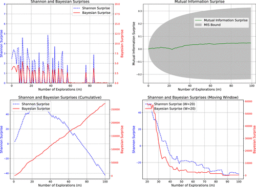
4.1.1. Scenario 1: Standard Exploration.
New data are randomly sampled from , expanding the domain while adhering to the same underlying response function in Equation (11). As the sampling region broadens, the input distribution evolves, which in turn alters the joint distribution and the observed functional relationship . Notably, this observed mapping may differ from the true system mapping in sparsely explored regions, where it is effectively inferred through extrapolation rather than direct observation.
This setting exemplifies a well-regulated autonomous system as defined in Definition 1: Although the joint distribution and the observed mapping evolve over time, the underlying input-output relationship, and thus the mutual information , remains stable.
Expected behavior: Because the system is well regulated, a meaningful surprise measure should not react to exploration-driven distributional shifts. In particular, variations in and the induced changes in should not be interpreted as unexpected events. Accordingly, we do not expect MIS to be violated.
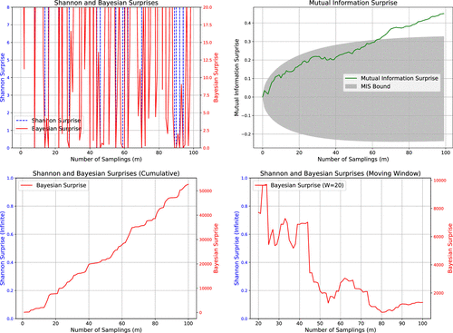
As shown in Figure 1, MIS evolves steadily within its expected bounds, reflecting stable learning despite continuous changes in the observed data distribution. In contrast, the single-instance Shannon and Bayesian surprises fluctuate erratically, frequently producing spikes that lack clear interpretability. Their cumulative and rolling variants, although smooth, tend to exhibit largely monotonic trends that offer little actionable insight for decision making. Notably, the cumulative Shannon surprise shows a pivot around 25 sampling steps, which can be attributed to increased coverage of the sampling space: As the model becomes more familiar with the environment, familiar observations begin to dominate and outweigh unseen observations in new samples.
4.1.2. Scenario 2: Overexploitation.
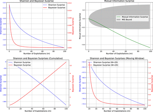
In this scenario, the system repeatedly samples a previously seen point from , specifically observing the pair 100 times. This simulates stagnation.
Expected behavior: Surprise should diminish as no new information is gained. This mirrors the stagnation case in Section 3.3, and we expect MIS to violate its lower bound.
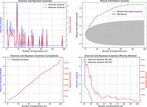
Figure 2 shows that MIS falls below its lower bound, clearly signaling a lack of knowledge gain. Although single-instance Shannon and Bayesian surprises also exhibit a downward trend, they lack a principled lower threshold, limiting their ability to reliably detect such behavior. As noted in Zamiri-Jafarian and Plataniotis (2022) and Ahmed et al. (2025), both Shannon and Bayesian surprises are inherently one-sided measures, which further constrains their interpretability. Similar patterns are observed for their multi-instance variants, with one notable exception: Cumulative Bayesian surprise increasingly labels the exploitation behavior as more surprising over time, whereas rolling Bayesian measures deem it progressively less surprising. Nevertheless, due to its KL divergence formulation, Bayesian surprise lacks a clear probabilistic threshold, rendering this trend difficult to translate into actionable signals.
4.1.3. Scenario 3: Noisy Exploration.
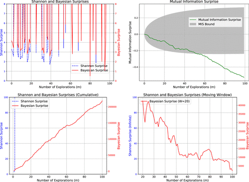
We perform standard exploration over but apply random corruption to the outputs , replacing each with a uniformly random digit between zero and nine. This simulates exploration without informative feedback.
Expected behavior: Despite novel inputs, the system should register confusion if understanding fails to improve. This mirrors the noise-increase case in Section 3.3, and we expect MIS to violate its lower bound.
Figure 3 confirms this pattern: MIS drops below its expected range, accurately signaling knowledge loss. In contrast, Shannon and Bayesian surprises again exhibit erratic behavior without consistent trends. Meanwhile, the multi-instance Shannon surprise diverges to infinity, and the cumulative and rolling variants of Bayesian surprise display contradictory monotonic patterns, further limiting their interpretability and practical usefulness.
4.1.4. Scenario 4: Aggressive Exploration.
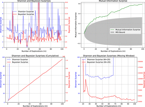
This scenario enforces strict exploration over , where each new sample is far from all observed points (i.e., outside the neighborhood range).
Expected behavior: Aggressive exploration without verification can lead to overconfidence. This mirrors the aggressive exploration case in Section 3.3, and we expect MIS to exceed its upper bound.
Figure 4 shows MIS exceeding its upper bound, consistent with the expected behavior under pure exploration. In contrast, the single-instance Shannon and Bayesian surprises again fluctuate unpredictably. The multi-instance Shannon surprise diverges to infinite values, whereas the cumulative and rolling versions of Bayesian surprise once more exhibit contradictory monotonic trends, limiting their interpretability.
4.1.5. Scenario 5: Noise Decrease.
To simulate noise reduction, we begin with 100 initial observations from , paired with a randomly assigned output . New samples are drawn from the same x range but the new y is produced using the deterministic modulus function in Equation (11).
Expected behavior: Reduced noise implies stronger input-output dependency, and we thus expect MIS to exceed its upper bound.
Figure 5 confirms this: MIS grows beyond its bound. Shannon and Bayesian surprises show similar behaviors to the prior scenarios.
4.1.6. Scenario 6: Discovery of New Output Values.
We modify the function in the unexplored region () to , introducing a different behavior while keeping the original function unchanged in [0, 30].
Expected behavior: A competent surprise measure should register this new structure as a meaningful discovery. This mirrors the novel discovery case in Section 3.3, and we expect MIS to exceed its upper bound.
Figure 6 shows MIS sharply exceeding its expected trajectory, signaling successful identification of a structural shift. Shannon and Bayesian surprises again fail to provide consistent or interpretable responses.
4.1.7. Summary.
Across all scenarios, MIS reliably indicates whether the system is genuinely learning, stagnating, or encountering degradation. It responds to the structure and value of observations, more than just novelty. In contrast, single-instance Shannon and Bayesian surprises often react to superficial fluctuations and display numerical instability, and multi-instance Shannon and Bayesian surprises often exhibit simple and even contradictory (cumulative versus rolling) monotone behaviors. Furthermore, the MIS progression bound remains consistent and interpretable across all scenarios, whereas Shannon and Bayesian surprises lack a universal scale or threshold, as reflected by their inconsistent magnitudes across Figures 1–6. This inconsistency limits their effectiveness as a reliable trigger. Overall, this simulation study demonstrates MIS not only as a novel metric for quantifying surprise, but also as a more trustworthy indicator of learning dynamics—making it a promising tool for autonomous system monitoring.
Table 2 summarizes the differences between MIS and the Shannon and Bayesian family of surprises.
|
Table 2. Perspective Differences Among Shannon Family Surprises, Bayesian Family Surprises, and MIS
| Surprise | Single instance focused | Capture transient changes | Aware of learning progression | Parametric predictive modeling |
|---|---|---|---|---|
| Shannon Family | ✓ | ✗ | ✗ | ✗ |
| Bayesian Family | ✓ | ✗ | ✗ | ✓ |
| MIS | ✗ | ✓ | ✓ | ✗ |
4.2. Pollution Estimation: A Case Study
To demonstrate the practical utility of our proposed MIS reaction policy, we apply it to a real-time pollution map estimation scenario. We evaluate the impact of integrating the MIS reaction policy on system performance in a dynamic, nonstationary environment. Specifically, we compare two approaches: a selection of baseline sampling strategies and the same strategies governed by our MIS reaction policy.
4.2.1. Data Set: Dynamic Pollution Maps.
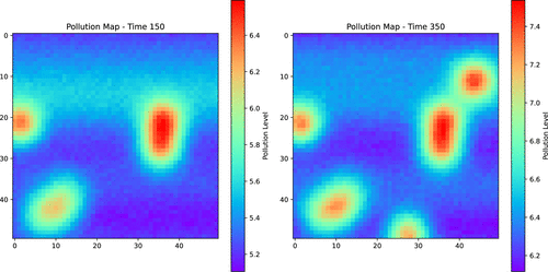
We utilize a synthetic pollution simulation data set comprising 450 time frames, each representing a pollution grid. Initially, the environment contains three pollution sources, each emitting high pollution at a fixed level. The rest of the field exhibits moderate and random pollution values. Over time, the pollution levels across the entire field evolve due to natural diffusion, decay, and wind effects. Moreover, every 50 frames, a new pollution source is added to the field at a random location. These new sources elevate the overall pollution levels and alter the input-output relationship between the spatial coordinates and the pollution intensity. Figure 7 displays a snippet of the pollution map at two intermediate time points. The simulation details for the dynamic pollution map generation are provided in the Online Appendix.
4.2.2. Sampling Strategies.
As discussed in Section 3.4, the MISRP is designed as a data-stream management mechanism that complements existing exploration-exploitation strategies. To evaluate its effectiveness, we conduct simulations using three well-established sampling strategies: the surprise-reactive (SR) sampling method proposed by Ahmed et al. (2025), implemented with either Shannon or Bayesian surprises; the subtractive clustering/entropy (SC/E) active learning strategy introduced by Cebron and Berthold (2009); and the greedy search/query-by-committee (GS/QBC) active learning strategy used in Islam et al. (2025). In addition, input-output data stream management has long been studied in the concept drift and anomaly detection literature. Accordingly, we compare MISRP against one of the most widely used cumulative drift detection metrics, the cumulative Shannon surprise (CSS) defined in Equation (12). Following standard practices in concept drift detection, once CSS exceeds a predefined threshold (), corresponding to the product likelihood falling below 0.1, previously collected data are discarded. Note that we do not benchmark the cumulative Bayesian surprise because, unlike the Shannon surprise, the KL divergence nature of the Bayesian surprise makes its triggering threshold ill defined, prohibiting the design of a reaction mechanism.
SR: The surprise-reactive sampling method (Ahmed et al. 2025) switches between exploration and exploitation modes based on the observed Shannon or Bayesian surprise. By default, SR operates in an exploration mode guided by the widely used space-filling principle (Joseph 2016), selecting new sampling locations via the min-max objective:
where denotes the set of existing observations. Upon encountering a surprising event (in terms of either the Shannon or Bayesian surprise), SR switches to exploitation mode, performing localized verification sampling within the neighborhood of the surprise-triggering location. This continues either for a fixed number of steps defined by an exploitation limit t, or until an unsurprising event occurs. If exploitation confirms that the surprise is consistent (i.e., persistent surprise until reaching the exploitation threshold), all corresponding observations are accepted and incorporated into the pollution map estimation. Conversely, if an unsurprising event arises before the threshold is reached, the surprising observations are deemed anomalous and discarded. For the Shannon surprise, we set the triggering threshold at 1.3, corresponding to a likelihood of . For the Bayesian surprise, we use the postdictive surprise and adopt the threshold of 0.5, following Ahmed et al. (2025).MISRP: The MISRP modifies SR by dynamically adjusting the exploitation limit t. When increased exploitation is needed, t is incremented by one. For increased exploration, t is decremented by one, with a lower bound of .
SC/E: The subtractive clustering/entropy active learning strategy (Cebron and Berthold 2009) selects the next sampling location by maximizing a custom acquisition function. For an unseen region and a probabilistic predictive function trained on the observed data, the acquisition function is defined as
where is the exploitation parameter, with a default value of 0.5, and denotes the entropy of the predictive distribution at . A larger value of emphasizes sampling at locations with high predictive uncertainty near previously seen points, promoting exploitation. A smaller value favors sampling at representative locations in the unseen region, promoting exploration (Cebron and Berthold 2009).MISRP: The MISRP modifies SC/E by adjusting the exploitation parameter . For increased exploitation, is increased by 0.1, up to a maximum of 1. For increased exploration, is decreased by 0.1, with a minimum of 0.
GS/QBC: The greedy search/query by committee active learning strategy (Islam et al. 2025) uses a different acquisition function. Given the set of seen observations and a model committee composed of multiple predictive models trained on these data, the acquisition function is defined as
(13)
MISRP: The MISRP regulates the balance between exploration and exploitation in GS/QBC in the same manner as in SC/E, by adjusting the parameter .
4.2.3. Experimental Setup.
The estimation process is initialized with 10 observed locations uniformly sampled across the pollution field. Each time frame collects 10 new samples according to the chosen sampling strategy, representing the operation of 10 mobile pollution sensors. The pollution field is estimated using a Gaussian process regressor with a Matérn kernel () and a noise prior of , consistently applied across all strategies. The model predicts pollution levels at specified spatial locations and is updated using both current and historical data, with a maximum of 200 observations retained to reduce computational cost.
For the GS/QBC strategy, the model committee additionally includes regressors with a Matérn kernel and a Gaussian kernel with bandwidth 0.1, both using a noise prior of . These two additional models are used solely for calculating disagreement in Equation (13) and are not employed in pollution map estimation.
The Shannon and Bayesian surprises are computed following the procedure described in Section 4.1. For MIS calculations, we discretize the range of pollution values observed in the data into 100 bins to estimate entropy, and we set the triggering probability at .
In process forking scenarios, two separate pollution map estimates, and , are produced for subprocesses and , respectively. The final pollution map estimate is formed as a weighted combination:
4.2.4. Simulation Results.
We assess performance using the mean squared error (MSE) between predicted and true pollution maps at each time step. Because of the dynamic nature of the pollution field, estimation errors exhibit substantial fluctuation. To smooth these variations, we compute a 20-frame moving average of the MSE for both vanilla and MISRP-governed strategies. The results are shown in Figure 8.
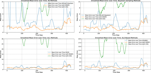
Notes. (Top left) SR with Shannon surprise. (Top right) SR with Bayesian surprise. (Bottom left) SC/E. (Bottom right) GS/QBC.
Across all comparisons, the baseline strategies display considerable volatility. In contrast, MISRP-governed counterparts produce smoother and consistently lower error curves, highlighting the stabilizing effect of MIS through its ability to facilitate adaptive responses in dynamic environments. CSS on the other hand, is constantly triggered, leaving very few observations for estimation, thus resulting in much higher estimation error and even higher volatility than the baseline strategies.
Table 3 presents the average estimation errors and their corresponding standard errors. The standard error is measured across 10 Monte Carlo simulations and 450 frames. Across all sampling strategies, incorporating the MIS reaction policy yields a substantial reduction in both mean estimation error and variability. Improvements in estimation error (compared with baseline strategies) range from to , whereas reductions in standard error range from to . On the other hand, CSS shows considerable performance degradation even compared with baseline strategies, highlighting the potential negative impact of traditional concept drift detection policy in this inherently dynamic process. The quantitative results in Table 3 highlight the impact of MISRP on learning performance, demonstrating substantial improvements in estimation accuracy and stability through data stream control.
|
Table 3. Comparison of Pollution Map Estimation Errors: Baseline vs. MISRP vs. CSS
| Sampling strategy | Estimation error (baseline) | Estimation error (CSS) | Estimation error (MISRP) | Mean improvement (over baseline) | Standard error improvement (over baseline) |
|---|---|---|---|---|---|
| SR with Shannon | |||||
| SR with Bayesian | |||||
| SC/E | |||||
| GS/QBC |
Note. Bold entries indicate the best performance.
To further illustrate the advantage of MISRP, we increase the per-frame sampling budget and the initial number of observed locations of the baseline strategies from 10 to 25, and expand the total memory buffer from 200 to 500, in order to assess whether baseline strategies can match the performance of MISRP-governed approaches. Table 4 compares the estimation error of MISRP-governed strategies (maintaining the original sampling budget of 10) against the enhanced baseline strategies. Even with a 2.5× increase in sampling budget, the baseline strategies remain significantly outperformed by their MISRP-governed counterparts.
|
Table 4. Error Comparison Under Extended Sampling for Baseline Strategies
| Sampling strategy | Estimation error (MISRP-governed, budget 10) | Estimation error (Baseline, budget 25) |
|---|---|---|
| SR with Shannon | 6.23 | |
| SR with Bayesian | 2.72 | |
| SC/E | 1.89 | |
| GS/QBC | 2.00 |
Note. Bold entries indicate the best performance.
Thus far, we demonstrated that governing basic sampling strategies with MISRP can substantially enhance learning performance in dynamic environments. To provide a clearer view of how MISRP operates over time, we conduct an additional simulation examining its actions throughout the process.
In this experiment, we simulate a two-phase pollution map evolution governed by the same PDE used in earlier simulation. During the first phase (time 0–250), three pollution sources emit high levels of pollutants, and the map evolves under diffusion, decay, and wind effects. At time step 250, the emission sources are removed, and the decay factor is reduced to 1/20th of its original value. The system then continues evolving for an additional 50 steps.
When the pollution sources exist and are emitting (the dynamic phase, time 0–250), the underlying process is a nonstationary process in which we expect frequent MIS triggering. When the pollution sources are gone (the stationary phase, time 251–300), the pollutants in the area will eventually diffuse to a stationary existence, during which time MIS is expected to stop being triggered.
Figure 9 shows the estimation error progression with action overlays under surprise-reactive sampling based on Shannon surprise. Recall from Section 3.4 that there are two actions employed in MISRP governance: sampling adjustments and process forking. These two actions are marked as vertical lines and shaded regions in the plot, respectively. For clarity, we present the 20-frame moving average of estimation error, whereas the nonsmooth version is provided in the Online Appendix. Actions are displayed 20 steps in advance, corresponding to their first observable effect on the smoothed error trajectory.
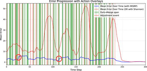
Several key observations emerge from the figure. First, both sampling adjustments and process forking occur frequently during the dynamic phase as expected, highlighting the effectiveness of MISRP’s action design in maintaining low estimation error. Second, sudden spikes in estimation error (circled) under MISRP governance are almost always followed by corrective actions that prevent further error growth, resulting in nonsmooth error progressions after intervention. By contrast, the baseline sampling strategy allows estimation error to rise unchecked. Then, once the system enters the stationary phase, MISRP ceases intervention, aligning with the intuition that a balanced sampling strategy in a well-regulated system should not trigger MIS.
5. Conclusion
We started the paper by presenting a vivid picture of the recent race toward autonomous systems. We argued that, although the bodies of various autonomous system have advanced visibly, over the past decade, the brains of these autonomous systems still miss a critical element, which is how to define and react to surprises. Unlike classical surprise measures that characterize statistical irregularities, we reimagine the concept of surprise as a mechanism for fostering understanding. We further define a new surprise metric based on mutual information and reframe surprise as a reflection of learning progression grounded in mutual information growth.
We developed a formal test sequence to monitor deviations in the estimated mutual information and introduced a reaction policy, MISRP, that transforms surprise into actionable system behavior. Through a synthetic case study and a pollution map estimation task, we demonstrated that MIS governance offers clear advantages over conventional sampling strategies. Our results show improved stability, better responsiveness to environmental drift, and significant reductions in estimation error. These findings affirm MIS as a robust and adaptive supervisory signal for autonomous systems.
Looking forward, this work opens several promising directions for future research. A natural next step is the development of a continuous space formulation of mutual information surprise, enabling its application in large complex systems. Another direction involves designing a specialized reaction policy—one that incorporates a sampling strategy tailored directly to the structure and signals of MIS, rather than relying on existing sampling strategies. This could enhance efficiency and responsiveness in highly dynamic or resource-constrained systems. Moreover, pairing MIS with physical probing capability for specific physical systems could unlock the true potential of MIS, as MIS provides new perspectives in system characterization compared with traditional measures.
References
- (2025) Toward futuristic autonomous experimentation—A surprise-reacting sequential experiment policy. IEEE Trans. Automation Sci. Engrg. 22:7912–7926.Google Scholar
- (2020)
Anomaly detection at scale: The case for deep distributional time series models . Proc. Internat. Conf. Service-Oriented Comput. (Springer, Berlin, Heidelberg), 97–109.Google Scholar - (2018)
Clustering and unsupervised anomaly detection with l-2 normalized deep auto-encoder representations . Proc. Internat. Joint Conf. Neural Networks (IEEE, Piscataway, NJ), 1–6.Google Scholar - (2002) A computational theory of surprise. Blaum M, Farrell PG, eds. Proc. Workshop Honoring Prof. Bob Mceliece on His 60th Birthday: Inform., Coding and Math. (Springer, Berlin, Heidelberg), 1–25.Google Scholar
- (2013) Novelty or surprise? Frontiers Psych. 4:907.Google Scholar
- (2022) From concept drift to model degradation: An overview on performance-aware drift detectors. Knowledge Based Systems 245:108632.Google Scholar
- (2009) Discriminative learning under covariate shift. J. Machine Learn. Res. 10(9):2137–2155.Google Scholar
- (2022) Anomaly detection in autonomous driving: A survey. Proc. IEEE/CVF Conf. Comput. Vision Pattern Recognition (IEEE, Piscataway, NJ), 4487–4498.Google Scholar
- (2010) Exploration vs. exploitation in active learning: A Bayesian approach. Proc. Internat. Joint Conf. Neural Networks (IEEE, Piscataway, NJ), 1–7.Google Scholar
- (2020) A mobile robotic chemist. Nature 583:237–241.Google Scholar
- (2020) Anomaly detection for autonomous guided vehicles using Bayesian surprise. Proc. IEEE/RSJ Internat. Conf. Intelligent Robots Systems (IEEE, Piscataway, NJ), 8148–8153.Google Scholar
- (2009) Active learning for object classification: From exploration to exploitation. Data Mining Knowledge Discovery 18:283–299.Google Scholar
- (2009) Generalization errors and learning curves for regression with multi-task Gaussian processes. Proc. 23rd Adv. Neural Inform. Processing Systems (ACM, New York), 279–287.Google Scholar
- (2020) Efficient closed-loop maximization of carbon nanotube growth rate using Bayesian optimization. Sci. Rep. 10:9040.Google Scholar
- (2015) Active hypothesis testing for anomaly detection. IEEE Trans. Inform. Theory 61(3):1432–1450.Google Scholar
- (1999) Elements of Information Theory (John Wiley & Sons, New York).Google Scholar
- (2024) Autonomous mobile robots for exploratory synthetic chemistry. Nature 635:890–897.Google Scholar
- (1984) Present position and potential developments: Some personal views statistical theory the prequential approach. J. Roy. Statist. Soc.: Ser. A (General) 147(2):278–290.Google Scholar
- (2023) Measuring surprise in the wild. Preprint, submitted May 12, https://arxiv.org/abs/2305.07733.Google Scholar
- (2013) Mutual information-based feature selection for multilabel classification. Neurocomputing 122:148–155.Google Scholar
- (2018) Balancing new against old information: The role of puzzlement surprise in learning. Neural Comput. 30(1):34–83.Google Scholar
- (2006) The permutation test for feature selection by mutual information. Proc. 14th Eur. Sympos. Artificial Neural Networks (ESANN, Bruges, Belgium), 239–244.Google Scholar
- (2015) Active inference and epistemic value. Cognitive Neurosci. 6(4):187–214.Google Scholar
- (2020) Mahalanobis distance based adversarial network for anomaly detection. Proc. IEEE Internat. Conf. Acoustics, Speech and Signal Processing (IEEE, Piscataway, NJ), 3192–3196.Google Scholar
- (2025) Dynamic exploration–exploitation trade-off in active learning regression with Bayesian hierarchical modeling. IISE Trans. 57(4):393–407.Google Scholar
- (2009) Bayesian surprise attracts human attention. Vision Res. 49(10):1295–1306.Google Scholar
- (2022) Autonomous experimentation systems and benefit of surprise-based Bayesian optimization. Proc. Internat. Sympos. Flexible Automation (ASME, Yokohama, Japan), 1–7.Google Scholar
- (2016) Space-filling designs for computer experiments: A review. Quality Engrg. 28(1):28–35.Google Scholar
- (2023) Null hypothesis test for anomaly detection. Phys. Lett. B 840:137836.Google Scholar
- (2015) A computational analysis of the neural bases of Bayesian inference. Neuroimage 106:222–237.Google Scholar
- (2020) Repad: Real-time proactive anomaly detection for time series. Proc. Internat. Conf. Advanced Inform. Networking Appl. (Springer), 1291–1302.Google Scholar
- (2023) Towards resilience in industry 5.0: A decentralized autonomous manufacturing paradigm. J. Manufacturing Systems 71:95–114.Google Scholar
- (2011) Towards fully autonomous driving: Systems and algorithms. Proc. IEEE Intelligent Vehicles Sympos (IEEE, Piscataway, NJ), 163–168.Google Scholar
- (2021) Learning in volatile environments with the Bayes factor surprise. Neural Comput. 33(2):269–340.Google Scholar
- (2022) Anomaly detection and correction of optimizing autonomous systems with inverse reinforcement learning. IEEE Trans. Cybernetics 53(7):4555–4566.Google Scholar
- (2020) Self-driving laboratory for accelerated discovery of thin-film materials. Sci. Adv. 6(20):eaaz8867.Google Scholar
- (2023) Scaling deep learning for materials discovery. Nature 624:80–85.Google Scholar
- (2022) A taxonomy of surprise definitions. J. Math. Psych. 110:102712.Google Scholar
- (2016) Artificial immune system via Euclidean distance minimization for anomaly detection in bearings. Mechanical Systems Signal Processing 76:380–393.Google Scholar
- (2012) A unifying view on dataset shift in classification. Pattern Recognition 45(1):521–530.Google Scholar
- (2019) Anomaly detection with multiple-hypotheses predictions. Proc. 36th Internat. Conf. Machine Learn., Proceedings of Machine Learning Research, vol. 97 (PMLR, New York), 4800–4809.Google Scholar
- (2016) Autonomy in materials research: A case study in carbon nanotube growth. NPJ Comput. Material 2:16031.Google Scholar
- (2003) Estimation of entropy and mutual information. Neural Comput. 15(6):1191–1253.Google Scholar
- (2012) An autonomous manufacturing system based on swarm of cognitive agents. J. Manufacturing Systems 31(3):337–348.Google Scholar
- (2021) Human inference in changing environments with temporal structure. Psych. Rev. 128(5):879–912.Google Scholar
- (2024) An augmented surprise-guided sequential learning framework for predicting the melt pool geometry. J. Manufacturing Systems 75:56–77.Google Scholar
- (2021) High-tech defense industries: Developing autonomous intelligent systems. Appl. Sci. 11(11):4920.Google Scholar
- (1993) Alternatives to the median absolute deviation. J. Amer. Statist. Assoc. 88(424):1273–1283.Google Scholar
- (2019) F-anoGAN: Fast unsupervised anomaly detection with generative adversarial networks. Medical Image Anal. 54:30–44.Google Scholar
- (1948) A mathematical theory of communication. Bell System Tech. J. 27(3):379–423.Google Scholar
- (2007) Covariate shift adaptation by importance weighted cross validation. J. Machine Learn. Res. 8(5):985–1005.Google Scholar
- (2023) An autonomous laboratory for the accelerated synthesis of novel materials. Nature 624:86–91.Google Scholar
- (1994) Generalizing the Fano inequality. IEEE Trans. Inform. Theory 40(4):1247–1251.Google Scholar
- (2013) Online anomaly detection for hard disk drives based on Mahalanobis distance. IEEE Trans. Reliability 62(1):136–145.Google Scholar
- (2014) A survey of distance and similarity measures used within network intrusion anomaly detection. IEEE Comm. Surveys Tutorials 17(1):70–91.Google Scholar
- (2020) A survey of autonomous driving: Common practices and emerging technologies. IEEE Access 8:58443–58469.Google Scholar
- (2022) A Bayesian surprise approach in designing cognitive radar for autonomous driving. Entropy 24(5):672.Google Scholar
- (2023) Concept drift monitoring and diagnostics of supervised learning models via score vectors. Technometrics 65(2):137–149.Google Scholar
- (2016) Continuous anomaly detection in satellite image time series based on z-scores of season-trend model residuals. Proc. IEEE Internat. Geosci. Remote Sensing Sympos. (IEEE, Piscataway, NJ), 3410–3413.Google Scholar
- (2016)
An overview of concept drift applications . Big Data Analysis: New Algorithms New Society 16: 91–114.Google Scholar

