


Arcflow Formulations and Constraint Generation Frameworks for the Two Bar Charts Packing Problem
Abstract
We consider the two bar charts packing problem (2-BCPP), a recent combinatorial optimization problem whose aim is to pack a set of one-dimensional items into the minimum number of bins. As opposed to the well-known bin packing problem, pairs of items are grouped to form bar charts, and a solution is only feasible if the first and second items of every bar chart are packed in consecutive bins. After providing a complete picture of the connections between the 2-BCPP and other relevant packing problems, we show how we can use these connections to derive valid lower and upper bounds for the problem. We then introduce two new integer linear programming (ILP) models to solve the 2-BCPP based on a nontrivial extension of the arcflow formulation. Even though both models involve an exponential number of constraints, we show that they can be solved within a constraint generation framework. We then empirically evaluate the performance of our bounds and exact approaches against an ILP model from the literature and demonstrate the effectiveness of our techniques on both benchmarks inspired by the literature and new classes of instances that are specifically designed to be hard to solve. The outcomes of our experiments are important for the packing community because they indicate that arcflow formulations can be used to solve targeted packing problems with precedence constraints and also that some of these formulations can be solved with constraint generation.
History: Accepted by Andrea Lodi, Area Editor for Design & Analysis of Algorithms–Discrete.
Supplemental Material: The online supplement is available at https://doi.org/10.1287/ijoc.2022.1256.
1. Introduction
Given a set of weighted items and an unlimited number of identical capacitated bins, the bin packing problem (BPP) requires packing all the items into the minimum number of bins. The BPP was introduced several decades ago by Kantorovich (1960) and quickly became one of the most studied combinatorial optimization problems. Indeed, its relatively simple structure made it the perfect playground for the research community to develop and test the most effective solution methods, including branch-and-bound algorithms (Martello and Toth 1990), metaheuristics (Falkenauer 1996), branch-and-price algorithms (Vance 1998), pseudo-polynomial formulations (Valério de Carvalho 1999), constraint programming (Shaw 2004), and reinforcement learning (Cai et al. 2019). Besides theoretical motivations, the BPP is also studied for its applications in the cutting industry (Stadtler 1990) and for its key role when solving more complex combinatorial optimization problems such as the vehicle routing problem (Lysgaard et al. 2004) and the two-dimensional BPP (Côté et al. 2021).
Along the years, many extensions of the BPP were introduced. We mention in particular (i) the BPP with conflicts (Muritiba et al. 2010) in which pairs of items cannot be packed in the same bin, (ii) the contiguous BPP (Martello et al. 2003) in which pairs of identical items must be packed in consecutive bins, and (iii) the vector packing problem (Brandão and Pedroso 2016) in which the item weights and bin capacities are multidimensional vectors and a capacity constraint is imposed on every dimension.
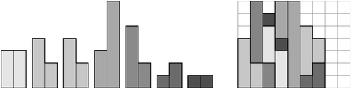
Erzin et al. (2021b) introduces one of the latest BPP extensions, which is known as the bar charts packing problem (BCPP). In the BCPP, we are given a set of ordered lists of weighted items (the bar charts) that must be packed using the minimum number of identical capacitated bins. Besides the usual capacity constraints, the BCPP also requires the items of a given bar chart to be packed in consecutive bins. The BCPP originates from a class of project scheduling problems in which one must determine the starting date (the bin) of a set of projects (the bar charts) so that the total makespan (the number of bins used) is minimized. Every project runs for a certain number of periods (one item in the bar chart corresponds to one period) and consumes a given amount of resource that may vary from one period to the other (the weights of the items in the bar chart). The total amount of resource available per period (the bin capacity) is limited, and once a project is started, it cannot be interrupted (contiguity constraints). In this paper, we are interested in the special case of the problem in which every bar chart is composed of exactly two items: the 2-BCPP. We show in Figure 1 a 2-BCPP instance (on the left part) together with a feasible packing that uses seven bins (on the right part).
Even though the 2-BCPP has a limited set of practical applications, it is still an interesting problem to study because it lies at the intersection of several well-known BPP extensions. It is, therefore, reasonable to assume that some of the most effective techniques aimed at solving these extensions can be adapted to solve the 2-BCPP. However, the available literature on the topic is mostly dedicated to approximation algorithms and their worst case performance ratio (Erzin et al. 2021a, b, c), whereas lower bounding procedures and exact approaches have not been thoroughly investigated.
1.1. Our Contribution
We provide an overview of the most relevant packing problems and cluster these problems into three classes , and . We show that
Every problem is a relaxation of the 2-BCPP, and thus, algorithms aimed at solving pl can also be used to derive valid lower bounds for our problem.
The 2-BCPP is a relaxation of every problem , and thus, algorithms aimed at solving pu can also be used to derive valid upper bounds for our problem.
The 2-BCPP is a special case of every member , and thus, algorithms aimed at solving pe can also be used to solve our problem, but the current state-of-the-art approaches are not well-suited for large-sized 2-BCPP instances.
We then introduce Eulerian-flow and link-flow, two new integer linear programming (ILP) models based on the well-known arcflow formulation introduced by Valério de Carvalho (1999) for the BPP. As both models use a pseudo-polynomial number of variables and an exponential number of constraints, we propose a constraint generation framework to solve each of these models to optimality.
Subsequently, we empirically evaluate the bounding procedures, the newly introduced decomposition approaches, and two methods proposed by Erzin et al. (2021b) (an ILP model and a heuristic) on a large set of random instances, and we identify instance features for which the tested approaches are particularly effective. For example, the ILP model of Erzin et al. (2021b) works very well when the maximum item weight is below a 10th of the bin capacity, whereas Eulerian-flow and link-flow are several orders of magnitude faster otherwise. We also design two new classes of hard instances for the 2-BCPP: TRIPLETS, in which the main difficulty is to find an optimal solution (i.e., find the right upper bound), and DONUTS, in which the main difficulty is to prove that the incumbent solution is optimal (i.e., find the right lower bound).
Besides making significant progress in the 2-BCPP field, the ideas we introduce are also relevant for arcflow formulations in general. In particular, to the best of our knowledge, it is the first time that an arcflow model is proposed for a BPP with a form of precedence constraints, indicating that similar approaches can be used for a larger set of packing problems. It is also the first time that an arcflow model is solved through constraint generation. This could lead to promising developments in decomposition approaches in which the master problem is a BPP (see e.g., the recent work of Côté et al. 2021 to solve the two-dimensional BPP). Indeed, arcflow formulations can now be considered to solve the master problem instead of the frequently used textbook (or “Kantorovich”) ILP model.
1.2. Related Work
The 2-BCPP is formally introduced by Erzin et al. (2021b). The authors propose several approximation algorithms with proven worst case performance ratios and compare the results obtained by their approaches to those obtained when solving a descriptive ILP model with the commercial solver CPLEX. They empirically show that the solver is more effective for instances with up to 100 bar charts, whereas the heuristics display better empirical performance otherwise. The ILP model considered by Erzin et al. (2021b) uses one variable per combination of bar chart and bin and is a direct extension of the textbook BPP model. Later on, Erzin et al. (2021a) perform additional experiments in which they use 2-BCPP instances with known optimal solutions to compute more accurate optimality gaps for the tested approaches. In a subsequent work, Erzin et al. (2021c) propose two additional approximation algorithms for special versions of the 2-BCPP and derive the associated worst case performance ratios. They study the case in which every bar chart contains at least one item with weight above half of the bin capacity and the case in which, in addition to that condition, the first item of every bar chart is at least as large as the second item.
Even though the 2-BCPP literature is relatively scarce, there are a few papers focusing on closely related packing problems that are particularly relevant for our study. In the following, we provide an overview of related problems together with a brief literature review and group them into three classes: (i) , the problems that are relaxations of the 2-BCPP; (ii) , the problems for which the 2-BCPP is a relaxation; and (iii) , the problems for which the 2-BCPP is a special case.
1.2.1. Problem Class .
Every packing problem that is a valid relaxation of the 2-BCPP belongs to . In other words, transforming a 2-BCPP instance I into an instance of problem and solving to optimality provides a valid lower bound for I. If we remove the constraints forcing the items of a given bar chart to be packed in consecutive bins, we obtain the BPP. The version of the BPP in which duplicate items are merged into a unique item with integer demand is called the cutting stock problem (CSP). A survey on heuristics and approximation algorithms for the BPP and the CSP is proposed by Coffman et al. (2013), whereas a survey focusing on exact approaches and mathematical models is presented by Delorme et al. (2016). Among the most effective approaches proposed in the literature, we mention branch-and-price algorithms (see Pessoa et al. 2020, Wei et al. 2020b) and pseudo-polynomial formulations (see Valério de Carvalho 1999, Brandão and Pedroso 2016, Delorme and Iori 2020). If we additionally forbid the two items of any bar chart to be packed in the same bin, we obtain the BPP with conflicts. Branch-and-price algorithms (see Sadykov and Vanderbeck 2013) and pseudo-polynomial formulations (see Brandão and Pedroso 2016) are also shown to be effective approaches for solving the BPP with conflicts. Finally, if we force the first item of a given bar chart to always be packed “before” the second item (i.e., in a bin with a lower index), we obtain the BPP with precedence constraints. So far, this problem is mostly tackled by branch-and-bound algorithms (see Dell’Amico et al. 2012, Pereira 2016) and branch-and-price algorithms (see Letelier et al. 2022).
1.2.2. Problem Class .
Every packing problem for which the 2-BCPP is a valid relaxation belongs to . In other words, transforming a 2-BCPP instance I into an instance of problem and solving to optimality provides a valid upper bound for I. If we force the first item of every bar chart to be packed in a bin with an odd index (i.e., if the first item of every bar chart can only be packed with other first items), we obtain the two-dimensional vector packing problem (2D-VPP). This problem is extensively studied in the literature and can be efficiently solved through tailored branch-and-price algorithms (see Wei et al. 2020a) and pseudo-polynomial formulations (see Brandão and Pedroso 2016). If, instead, we merge the two items of every bar chart into a two-dimensional item (i.e., if we force the bottom left corner of the two items in a given bar chart to have the same y-coordinate), we obtain a version of the strip packing problem in which the items can either be rectangles or “L-shaped” hexagons. Algorithms aimed at solving the classic strip packing problem (e.g., the Benders’ decomposition approaches from Côté et al. 2014, Delorme et al. 2017) can be extended to also take into account L-shaped hexagons.
1.2.3. Problem Class .
Every packing problem for which the 2-BCPP is a special case belongs to . In other words, transforming a 2-BCPP instance I into an instance of problem and solving to optimality provides an optimal solution for I. The 2-BCPP can be seen as a special case of the contiguous BPP, which is introduced by Martello et al. (2003) as a relaxation of the strip packing problem (SPP). In that relaxation, every two-dimensional item is cut into unit-height slices, and the objective is to find a packing that uses the minimum number of bins such that the slices originating from the same item are packed into contiguous bins. Even though the items involved in a contiguity constraint have the same weight in the SPP relaxation, one can also consider a version of the contiguous BPP in which this is not the case. In the literature, the contiguous BPP is tackled with ad hoc branch-and-bound algorithms (see Martello et al. 2003) and ILP models solved through commercial solvers (see Côté et al. 2014, Delorme et al. 2017). These ILP models can easily be extended to the 2-BCPP, but Erzin et al. (2021b) show that the resulting approaches are only able to solve small-sized instances to optimality.
The 2-BCPP is also a special case of the BPP with time lags recently introduced by Letelier et al. (2022). In that extension, two items involved in a time lag constraint have a minimum and a maximum time lag, which is defined as the difference between the index of the bins in which the two items are packed. In the version studied by Letelier et al. (2022), the minimum and maximum time lags can vary from one pair of items to the other and are not necessarily bounded. For example, one pair of items can be constrained to have a time lag in the range , whereas another pair can be constrained to have a time lag in the range . The 2-BCPP is, thus, a special case of the BPP with time lags in which every pair of items in a given bar chart is forced to have a time lag in the range . Letelier et al. (2022) propose two ILP models for the BPP with time lags: one that can be seen as an extension of the model proposed by Erzin et al. (2021b) and one that uses an exponential number of variables where each variable decides whether a given pattern is used in a bin with a given index. The latter model is solved with a branch-and-price algorithm and can handle instances with up to a few hundred items. Even though these approaches can also be used to solve the 2-BCPP, we do not expect them to work very well in practice because they need one set of variables per bin index, which quickly becomes impractical for large-sized instances. In this paper, we introduce two new ILP models that make use of the special structure of the 2-BCPP to avoid the necessity to take the bin index into account.
1.3. Layout
The remainder of this paper is structured as follows. In Section 2, we formally define the 2-BCPP, and we discuss the ILP model proposed by Erzin et al. (2021b). In Section 3, we briefly introduce existing arcflow formulations for the CSP and the 2D-VPP and outline how valid lower and upper bounds for the 2-BCPP can be obtained by solving these models. In Section 4, we introduce two new ILP models for our problem. Both of these models are based on the arcflow formulation, have an exponential number of constraints, and can be solved within a constraint generation framework. In Section 5, we present two innovative ways to construct difficult instances for the problem, and we report the findings of a large number of computational experiments. Finally, conclusions are drawn in Section 6.
2. Problem Definition
In the 2-BCPP, we are given an unlimited number of bins with capacity c and a set of n bar charts, each of them composed of two bars (or items—the terms are interchangeable) that must be packed in consecutive bins: the first bar whose weight is denoted by and the second bar whose weight is denoted by . We call the weight vector of bar chart i. For feasibility purposes, we assume that for every bar chart . We also assume that and c are strictly positive integers and that every bar chart has an integer demand qi. Note that, in the original 2-BCPP definition from Erzin et al. (2021b), every bar chart had demand one and bar weights were positive real numbers. However, an instance of such a problem can be transformed to fit our definition by merging duplicate bar charts, computing the associated demands, and multiplying the bar weights and the capacity by a suitable coefficient.
Given a 2-BCPP solution, we say that bar chart i is packed into bin j if the first item of bar chart i is packed into bin j (and, thus, if the second item of bar chart i is packed into bin j + 1). In addition, we say that a solution (or a packing) is feasible if the demand, the contiguity, and the capacity constraints are satisfied. We call z the length of a feasible packing, which is defined as the number of bins in the solution containing at least one item. For a feasible solution of length z, it is assumed that at least one item is packed in every bin . If this is not the case, one can simply delete the empty intermediate bins and shift the solution. Finally, we say that a feasible packing with length is optimal if there exists no solution with length z such that .
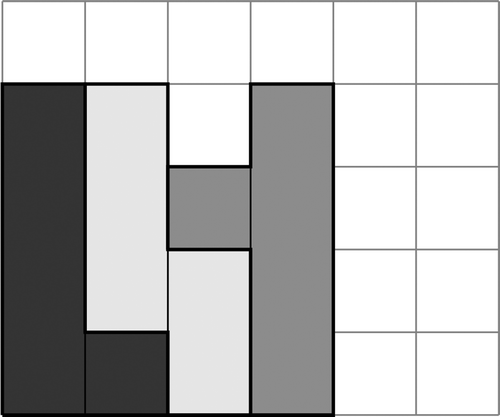
Let us consider the following 2-BCPP instance with n = 3, , and c = 5. An optimal packing is shown in Figure 2 in which the first bar chart is packed in bin 1 (i.e., its first and second items are packed in bins 1 and 2, respectively), the second bar chart is packed in bin 2, and the third bar chart is packed in bin 3. This solution has length as it uses four bins.
Let us consider a valid upper bound K on the minimum number of bins required to pack all the bar charts. A trivial value for K is . By introducing binary decision variables yj that take value one if bin j is opened and zero otherwise and integer decision variables xij that indicate the number of times bar chart i is packed into bin j , the 2-BCPP can be modeled as follows (Erzin et al. 2021b):
The objective function (1) minimizes the number of bins used, whereas Constraints (2) make sure that the bar chart demands are satisfied. Constraints (3)–(5) ensure that the sum of the item weights contained in a given bin never exceeds the bin capacity while also preventing any item to be packed in a closed bin (i.e., a bin whose corresponding yj variable is equal to zero). Finally, symmetry-breaking Constraints (6) make sure that the bins are opened from lowest to highest index (i.e., without intermediate empty bins) and Constraints (7) and (8) limit the variable domains. Model (1)–(8) uses O(nK) variables and constraints, which means that, for reasonably small n and K values, the model size should not be a problem. Yet we show in our computational experiments that instances with as few as 50 bar charts cannot be solved after one hour of computing time by a commercial ILP solver, which motivates the introduction of better formulations.
3. Arcflow-Based Lower and Upper Bounding Procedures
For many packing problems, researchers show that arcflow formulations provide much better results on average than “Kantorovich-like” models (see Delorme et al. 2016, Martinovic and Scheithauer 2016, Dell’Amico et al. 2019). The name “arcflow” originates from the fact that the variables in the model represent flows on individual arcs in a directed graph (see de Lima et al. 2022 for a recent survey on the topic). Arcflow formulations are known to have a very tight LP-relaxation, but this comes at the cost of not being polynomial in the input size. Indeed, both the number of variables and constraints involved in such models are usually polynomial in the capacity, whereas the latter is coded as bits in the input, which is why arcflow formulations are said to be pseudo-polynomial. There is a growing interest in the research community for arcflow formulations as (i) they are usually easy to implement as they do not involve advanced optimization techniques and (ii) they result in models that can often be solved to optimality with a state-of-the-art ILP solver, especially for instances with a reasonable capacity. In summary, arcflow models are seen as a good compromise between simplicity and efficiency.
Typically, an approach using an arcflow model is composed of three phases: (i) the graph-construction phase, in which the instance I of the original problem is transformed into an instance of a graph problem; (ii) the solving phase, in which the instance is solved (e.g., with an ILP solver); and (iii) the mapping phase, in which the solution of instance is mapped into a solution of instance I. In the following, we briefly introduce arcflow formulations for the CSP and 2D-VPP and explain how they can be used to derive valid lower and upper bounds for the 2-BCPP.
3.1. Arcflow-Based Lower Bounding Procedure
The idea behind the arcflow formulation for the CSP is introduced by Wolsey (1977) and popularized by Valério de Carvalho (1999). The CSP is transformed into a graph problem in which the objective is to minimize the flow going from a source node to a target node under demand and flow conservation constraints. In this section, n denotes the number of items in a CSP instance, wi is the weight of item i , and qi is the demand of the item.
In the graph-construction phase, we consider a graph , where vertex set and arc set for . Note that symmetry-reduction techniques can be used to reduce the size of V and A (see Valério de Carvalho 1999, Côté and Iori 2018).
In the solving phase, by introducing integer decision variables fde that indicate the number of times arc is selected, the arcflow model for the CSP can be defined as follows:
The objective function (9) minimizes the flow going from zero to c. Constraints (10) ensure that z units of flow both leave node 0 and enter node c, and enforce flow conservation in the other nodes. Constraints (11) make sure that the demand is satisfied, whereas Constraints (12) limit the variable domains.
In the mapping phase, a flow decomposition algorithm is used on the optimal solution of Model (9)–(12) to obtain a set of paths with unitary flow corresponding to an optimal CSP solution.
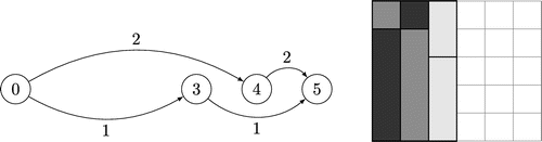
(Resumed). By splitting every bar chart in the 2-BCPP instance, we obtain a CSP instance in which , and c = 5. The optimal arcflow solution is depicted on the left part of Figure 3 and uses three bins: two bins containing an item with weight four and an item with weight one each and one bin containing an item with weight three and an item with weight two. Therefore, a valid lower bound for the original 2-BCPP instance is three. A graphic representation of the solution is shown on the right part of Figure 3.
3.2. Arcflow-Based Upper Bounding Procedure
The arcflow formulation for the 2D-VPP can be attributed to Brandão and Pedroso (2016), who extend the CSP version of the model to take into account additional dimensions. The 2D-VPP is again transformed into a graph problem in which the objective is to minimize the flow leaving a source node under demand and (a form of) flow conservation constraints. In this section, n designs the number of items in a 2D-VPP instance, (c1, c2) is the capacity of the bin, is the weight vector of two-dimensional item i , and qi is the demand of the item.
In the graph-construction phase, we consider a graph , where vertex set and arc set for . Note that symmetry-reduction techniques can also be used to reduce the size of V and A (see Brandão and Pedroso 2016). As it is relevant for the models introduced in the next section, we provide in Algorithm 1 in Section A of the online supplement a pseudo-code to construct graph G with a reduced vertex set V and a reduced arc set A.
In the solving phase, by introducing integer decision variables that indicate the number of times arc is selected, the arcflow model for the 2D-VPP can be defined as follows:
The objective function (13) minimizes the flow going out of node (0, 0). Constraints (14) ensure that the flow entering any node (v1, v2) that is not (0, 0) is never below the flow leaving that node. Constraints (15) make sure that the demand is satisfied, whereas Constraints (16) limit the variable domains.
In the mapping phase, a flow decomposition algorithm is used on the optimal solution of Model (13)–(16) to obtain a set of paths with unitary flow corresponding to an optimal 2D-VPP solution.
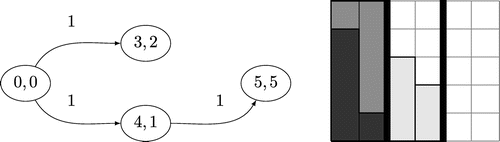
(Resumed). After converting the 2-BCPP instance, we obtain a 2D-VPP instance in which n = 3, , and . The optimal arcflow solution is depicted on the left part of Figure 4 and uses two bins: the first one containing items 1 and 3 and the second one containing item 2. Therefore, a valid upper bound for the original 2-BCPP instance is four as one bin in the 2D-VPP corresponds to two bins in the 2-BCPP. A graphic representation of the solution is shown on the right part of Figure 4.
4. New Arcflow Formulations for the 2-BCPP
Even if the arcflow formulation was originally proposed for the CSP, it has been successfully extended to many other relevant packing problems in the last two decades (see Macedo et al. 2010, Nesello et al. 2018, Delorme et al. 2021). In this section, we first introduce Eulerian-flow, a nontrivial arcflow extension for the 2-BCPP in which a feasible solution is represented by a single cycle in a graph (a Eulerian cycle). We observe that, whereas forcing the arcs selected in a solution to form cycles is relatively easy, making sure that these cycles are all connected (i.e., that there are no subtours) is much harder and can only be achieved by using an exponential number of constraints. As the model size quickly becomes too large to be solved by an ILP solver, we propose a constraint generation framework that only adds the subtour elimination constraints that are necessary to find an optimal solution. We then introduce link-flow, a model inspired by Eulerian-flow in which the number of variables is dramatically reduced at the cost of an extra set of constraints.
4.1. Eulerian-Flow
Our first model builds upon the arcflow formulation for the 2D-VPP described in the previous section in which a feasible packing is represented as a set of paths starting from node (0, 0). In that formulation, one can easily modify the arc set definition to incorporate feedback arcs for every to represent the end of a bin and updating flow conservation constraints (14) to
A feasible solution f now consists of a set of arcs that can be split into a number of cycles in which each cycle contains node (0, 0). Let us define the directed multigraph , also called the solution graph hereafter, in which Vf contains the set of vertices visited in solution f and Af contains copies of arc for every . According to Euler’s theorem (developed to solve the Königsberg bridge problem in 1736), a directed graph contains a Eulerian cycle if and only if (i) the in-degree of any vertex is equal to its out-degree and (ii) the graph is strongly connected. Solution graph Gf contains a Eulerian cycle as condition (i) is satisfied thanks to the updated flow conservation constraints (17), and condition (ii) is satisfied because the arcs in Af can be split into a set of cycles such that node (0, 0) is included in every cycle.
This updated formulation is not yet suitable for the 2-BCPP as it fills the bins by pairs, which means that it does not allow the first item of a bar chart to be packed with the second item of another bar chart. To correct this issue, we introduce transition arcs for every to represent the end of a 2-BCPP bin. Intuitively, one can see a transition arc as half of a feedback arc. In fact, using two successive transition arcs and is the same as using one feedback arc . We point out that, after introducing transition arcs, the arcs in Af can still be split into a set of cycles, but node (0, 0) is not necessarily included in each of these cycles anymore. This means that an additional set of constraints is required to make sure that the solution graph Gf is strongly connected (and, thus, that it contains a Eulerian cycle).
In the graph-construction phase, we consider a graph , where vertex set and arc set for . As the number of vertices and arcs grows quickly with c, we detail in the following how graph G can be constructed with a reduced vertex set V and a reduced arc set A. Note that, to avoid any confusion, we temporarily use different notation for the initial graph , the intermediate graph , and the final graph .
Order the bar charts (e.g., from the largest bar chart to the smallest).
Construct graph following Algorithm 1 in Online Section A.
Save in set Vh every distinct v2 value () such that for some v1.
Construct graph following a modified version of Algorithm 1 in which set V is initialized to Vh instead of and create and .
For every vertex , add transition arc to .
We point out that it is not necessary to update set Vh after the fourth step because every arc in has, by construction, its counterpart in , where . In fact, we can use this fact to generate and more efficiently by duplicating and “shifting” the first dimension of both the tail and the head of every arc by the values in Vh as described in Algorithm 2 in Online Section A. In the next phases, we refer to graph as the final graph built in this phase.
In the solving phase, for the sake of compactness, we now sometimes refer to an arc as a instead of . For every vertex , we also define index sets (respectively, ) as the set of arcs leaving (entering) vertex (v1, v2). For every , we denote by Ai the set of arcs representing the packing of a bar chart of type i (i.e., the set of arcs such that ). We call the set of bar chart arcs. We also denote by A0 the set of transition arcs. By introducing integer decision variables fa that indicate the number of times arc is selected, the Eulerian-flow model can then be defined as follows:
The objective function (18) minimizes the number of transition arcs used (i.e., the length of the packing). Constraints (19) ensure flow conservation, whereas Constraint (20) makes sure that there is at least one unit of flow leaving node (0, 0). Furthermore, Constraints (21) enforce demand satisfaction, and Constraints (22) eliminate subtours so that the solution graph Gf is strongly connected. More specifically, big-M constraints (22) ensure that, for every potential subtour (i.e., every subset of nodes that does not contain (0, 0)), there can only be a flow circulating in the subtour (i.e., in an arc whose tail and head are both in ) if there is also a flow leaving the subtour (i.e., passing through an arc whose tail is in and whose head is not in ). A suitable big-M value for Constraints (22) is as at most units of flow circulate in bar chart arcs and at most K units of flow circulate in transition arcs in total (we recall that K is an upper bound on the minimum number of bins). Note that we can decrease big-M values by making them constraint-specific. In that case, for the constraint associated with a given subset of nodes , we can remove the qi values of the bar charts for which there is no arc with both tail and head in . Model (18)–(23) uses variables and constraints.
In the mapping phase, after an optimal solution f is found for Model (18)–(23), we create the solution graph Gf and we find a Eulerian cycle in the graph starting in node (0, 0). Once such a cycle is obtained, we reconstruct a 2-BCPP solution by looping over every arc a in the Eulerian cycle and either inserting the bar chart associated with a into bin j if a is an item arc or incrementing j if a is a transition arc (j is initialized to one).
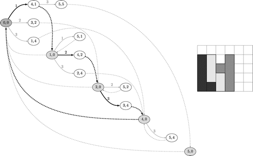
(Resumed). We solve the same 2-BCPP instance with n = 3, , and c = 5. The graph obtained after the graph-construction phase is depicted on the left part of Figure 5. Solid lines are bar chart arcs (the number on top of the arc is the bar chart index), and dashed lines are transition arcs. The solution obtained after the solving phase (e.g., given by an ILP solver) results in the flow f that is printed in bold and black on the left part of Figure 5 (every arc in f carries one unit of flow). To transform f into a valid 2-BCPP solution through the mapping phase, we identify Eulerian cycle , we initialize the bin index to one, and we start looping over every arc in the cycle. We pack bar chart 1 in bin 1 (i.e., its first item is packed in bin 1, and its second item is packed in bin 2), and then, we increment the bin index because the second arc is a transition arc. Then, we pack bar chart 2 in bin 2, we increment again the bin index, we pack bar chart 3 in bin 3, and we finish by incrementing the bin index twice. A graphic representation of the 2-BCPP solution is shown on the right part of Figure 5 and uses four bins.
Note that, for this instance, an optimal solution to Eulerian-flow without subtour elimination constraints has objective value three and is composed of two cycles: and . This solution satisfies flow conservation and demand constraints and has at least one unit of flow leaving node (0, 0). However, it cannot be mapped into a valid 2-BCPP solution as its associated solution graph does not contain a Eulerian cycle.
4.2. Constraint Generation Framework
A common way to solve ILP models that involve an exponential number of constraints is to use a constraint generation framework. The key idea behind constraint generation is to solve the formulation with a subset of constraints (e.g., with an ILP solver) and check if the returned solution is feasible for the initial problem (i.e., if the solution found also satisfies the constraints that were not included in ). If this is the case, then the solution is optimal. Otherwise, it means that at least one of the constraints not considered in the reduced model is important and needs to be added to . The process is iterated until an optimal solution is found. Note that constraint generation is very well-known in the routing community (see the work of Pferschy and Staněk 2017 on constraint generation for the traveling salesman problem).
A flowchart of our constraint generation framework is presented in Figure 6. After the graph-construction phase in which graph is generated, we solve the Eulerian-flow model without subtour elimination constraints to obtain a solution f. We then create the solution graph Gf, split the arcs of Af into the minimum number of disjoint cycles, and store the ones that do not contain node (0, 0) in . If , then f contains one or more subtours, and thus, cannot be mapped into a feasible 2-BCPP solution. As a result, a subtour elimination constraint is added to forbidding each of the subtours, and Eulerian-flow is solved once more with the updated subset . If , the algorithm stops as f can be mapped into a feasible 2-BCPP solution.

(Resumed). After solving the Eulerian-flow model without subtour elimination constraints, one can obtain a solution f containing subtour . Such a solution can be prevented from being generated again during the solving phase by adding subtour elimination constraint to (22).
We point out that, in state-of-the-art ILP solvers, constraint generation frameworks are usually implemented within callbacks (a set of functions created by the user that is called during the enumeration tree). In our callback implementation, every integer solution found by the solver is tested for subtours. If at least one subtour is found, relevant constraints are added to the solver, and the solution is, therefore, rejected. If no subtour is found, the solution becomes the new incumbent and the upper bound is, therefore, updated. In both cases, the solver continues its enumeration tree until the lower and upper bounds match.
4.3. Link-Flow
Even though reduction techniques are applied in the graph-construction phase of Eulerian-flow, preliminary tests show that the model size grows quickly as n and c increase even when the constraint generation framework is used. This is mainly because of the fourth step of the graph-construction phase in which the initial arc set is duplicated up to c – 1 times to allow any (ordered) combination of bar chart arcs to follow a transition arc. The key idea behind link-flow is to move the transition arc from the beginning of a bin to the end so that every bin now always starts from node (0, 0) and ends with a transition arc. Whereas the idea appears to be relatively simple and effective (as the duplication phase is no longer needed), its implementation is not necessarily trivial as we now need to make sure that the transition arcs “connect” to each other so that the bins form a feasible 2-BCPP solution. Intuitively, transition arcs can be seen as a set of pieces of a puzzle, and the subset we select needs to form a circle.
For the sake of clarity, we describe the link-flow model using two distinct graphs G1 and G2 (even though we will observe in the solving phase that building G2 is not strictly necessary). The primary graph G1 contains item arcs and link arcs (the counterpart of transition arcs in link-flow), whereas the secondary graph G2 contains link and loss arcs. Constraints in G1 make sure that the bins created are feasible and item requirements are satisfied. Constraints in G2 make sure that link arcs (and, thus, bins) can be combined together to form a feasible 2-BCPP solution (possibly with the help of loss arcs). This is done by ensuring that the secondary solution graph contains a Eulerian cycle. Supplementary constraints ensure that the link arcs selected in G1 and in G2 are the same.
In the graph-construction phase, the primary graph is initially constructed as the arcflow graph for the 2D-VPP (see Section 3.2 and Algorithm 1 in Online Section A). Link arcs are then added to A1 for every node . The secondary graph has vertex set and arc set in which the third index separates the link arcs (identified by “lk”) from the loss arcs (identified by “ls”).
In the solving phase, for every primary vertex , we still use as the set of primary arcs leaving (v1, v2) and as the set of primary arcs entering (v1, v2). Analogously, we define index sets and for every secondary vertex as the set of secondary arcs leaving and entering v. For every , we denote by the set of primary arcs representing the packing of a bar chart of type i. We call the set of bar chart arcs, and we denote by the set of link arcs in G1. By introducing integer decision variables () that indicate the number of times primary (secondary) arc () is selected, the link-flow model can then be defined as follows:
The objective function (24) minimizes the length of the packing. Constraints (25) and (26) enforce flow conservation in the primary and secondary graphs, whereas Constraint (27) makes sure that at least one unit of flow leaves secondary vertex 0. Furthermore, Constraints (28) ensure that the link arcs selected in G1 are the same as the link arcs selected in G2, Constraints (29) enforce demand satisfaction, and Constraints (30) eliminate subtours so that the solution graph is strongly connected. A suitable big-M value for Constraints (30) is K + Kc as at most K link arcs are selected in G1 (and, thus, in G2) and at most c loss arcs are required in G2 per link arc. Note that we can decrease big-M values by making them constraint-specific. In that case, for the constraint associated with a given subset of nodes , we can use the actual number of loss arcs having both tail and head in instead of the upper bound c. Model (24)–(32) uses variables and constraints. Note that we can reduce the model size even further by replacing variables associated with secondary link arcs by their counterpart in the primary graph and by removing Constraints (28). We can also use the constraint generation framework introduced previously to handle subtour elimination Constraints (30).
In the mapping phase, after an optimal solution is found for Model (24)–(32), we use a flow-decomposition algorithm to obtain a set of cycles with unitary flow in the primary graph. Each of these cycles corresponds to a bin, and we now need to order these bins. To do so, in the secondary graph, we create solution graph , and we find a Eulerian cycle starting from node 0. Note that is constructed as described in Eulerian-flow: , where contains the set of secondary vertices visited in solution f and contains copies of arc (d, e, l) for every . After initializing j to one, we reconstruct a 2-BCPP solution by looping over every arc a in the Eulerian cycle and inserting in bin j either one unit of loss space if a is a loss arc or the bar charts of the cycle that includes the counterpart of a in the primary graph otherwise. Index j is incremented every time a is a link arc.
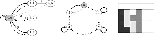
(Resumed). Consider again the running example. The primary and secondary graphs obtained after the graph-construction phase are depicted on the left and middle parts of Figure 7, respectively. In the primary graph, solid lines are bar chart arcs (the number on top of the arc is the bar chart index) and dashed lines are link arcs. In the secondary graph, solid lines are link arcs and dashed lines are loss arcs. Note that, as no secondary link arc starts or ends in three, loss arcs and are merged into . The solution obtained after the solving phase (e.g., given by an ILP solver) results in the flow that is printed in bold and black in the two graphs (every arc in f1 and f2 carries one unit of flow). To transform f into a valid 2-BCPP through the mapping phase, we first determine the cycles in the primary graph: , and . We then identify Eulerian cycle in the secondary graph. We pack one unit of loss space in bin 1 together with bar chart 1 as secondary link arc (1, 1) is associated with primary link arc . We increment the bin index and pack one unit of loss space in bin 2 together with bar chart 2 as secondary link arc (2, 2) is associated with primary link arc . We increment the bin index and pack two units of loss space in bin 3 together with bar chart 3 as secondary link arc (4, 4) is associated with primary link arc . We increment the bin index and pack one unit of loss space in bin 4. Finally, we increment the bin index and complete the Eulerian cycle with secondary link arc (5, 0), which is associated with primary link arc . A graphic representation of the 2-BCPP solution is shown on the right part of Figure 7 and uses four bins.
Note that, for this instance, an optimal solution to link-flow without subtour elimination constraints has objective value three and is composed of cycles and in the primary graph and and in the secondary graph. This solution satisfies flow conservation and demand constraints and has at least one unit of flow leaving secondary node 0. However, it cannot be mapped into a valid 2-BCPP solution as its associated solution graph does not contain a Eulerian cycle. By using the constraint generation framework, one can prevent such a solution from being generated again by adding subtour elimination constraint to (30).
5. Computational Experiments
We empirically evaluate the performance of each of the proposed approaches, namely,
CSP, the arcflow Model (9)–(12) described in Section 3.1 to obtain a lower bound.
EUL-REL, the Eulerian-flow Model (18)–(23) without subtour elimination Constraints (22) described in Section 4.1 to obtain a lower bound.
LINK-REL, the link-flow Model (24)–(32) without subtour elimination Constraints (30) described in Section 4.3 to obtain a lower bound.
2DV, the arcflow Model (13)–(16) described in Section 3.2 to obtain an upper bound.
ERZIN, Model (1)–(8) described in Section 2 introduced by Erzin et al. (2021b).
EUL-FLOW, the Eulerian-flow Model (18)–(23) in which subtour elimination constraints are added through the constraint generation framework described in Section 4.2.
LINK-FLOW, the link-flow Model (24)–(32) in which subtour elimination constraints are added through the constraint generation framework described in Section 4.2.
For comparative purposes, we also reimplement the best performing heuristic according to the experiments of Erzin et al. (2021b), GA_LO. It is a greedy approach that fills the bins one at a time by iteratively adding the bar chart with the largest first item among those fitting in the remaining space. When no bar chart can be packed into the current bin j, because either the first bar does not fit into bin j or the second bar does not fit into bin j + 1, then GA_LO closes bin j and starts filling bin j + 1. Our algorithms are all coded in C++ and can be downloaded from https://github.com/mdelorme2/Two_Bar_Charts_Packing_Problem. The experiments were run on an Intel(R) Core(TM) i7-4700MQ, 2.40 GHz with 8 GB of memory, running under Ubuntu 20.04.4 LTS, and Gurobi 9.5.0 was used to solve the ILP models. A single core was used for the tests (i.e., parameter Threads was set to one), the barrier algorithm was used to solve the root nodes of the ILP models (i.e., parameter Method was set to two), and callbacks were used for the constraint generation (and, thus, parameter LazyConstraints was set to one). In every instance, an upper bound K on the minimum number of bins required to pack the bar charts was obtained with a trivial first fit decreasing approach. For every run, a time limit of 3,600 seconds was imposed. We tested our approaches on six newly generated data sets with integer item weights and bin capacities, namely,
U-GEN, in which bar charts contain (a combination of) small, medium, and big items.
U-SMA, in which bar charts only contain small items.
U-MED, in which bar charts contain at least one medium item.
U-BIG, in which bar charts contain at least one big item.
TRIPLETS, in which an integer solution where every bin is entirely filled exists.
DONUTS, in which the bound derived from EUL-REL and LINK-REL is exactly one bin away from the optimal solution value.
Our data sets can be downloaded from https://github.com/mdelorme2/Two_Bar_Charts_Packing_Problem. For each data set, we first describe the instance-generation process and its motivation. We then empirically evaluate the performance of each of the aforementioned approaches, including an overview of the model size and quality of the LP relaxation.
5.1. Data Set Generation and Experiments on U-GEN, U-SMA, U-MED, and U-BIG
5.1.1. Data Set Generation.
In data sets U-GEN and U-SMA, the item weights of every bar chart are uniformly distributed in specific ranges: in U-GEN and in U-SMA. In data sets U-MED and U-BIG, the weight of one item of every bar chart (randomly selected between the first and second items) is uniformly distributed in , whereas the weight of the other item is uniformly distributed in in U-MED and in U-BIG. For each data set, we consider three distinct bin capacities and various numbers of bar charts (named Ω thereafter).
For c = 50, we tried .
For c = 100, we tried .
For c = 500, we tried .
For each of the 17 combinations, we generated 10 instances resulting in 170 instances in total per data set. To create an instance, we simply generated the desired Ω bar charts according to the specified distribution, and we merged the identical ones to obtain values n and qi .
5.1.2. Data Set Motivation.
Data sets similar to U-GEN and U-BIG were used in the experiments of Erzin et al. (2021a) on a standardized version of the 2-BCPP in which the bin capacity was always equal to one and the item weights were real numbers with up to eight digits after the decimal point. We decided to recreate these two data sets in order to have more flexibility over the capacity and the total number of bar charts. We also mention that there were some inconsistencies in the instance files we downloaded from the web link shared in Erzin et al. (2021a),1 which is another motivation for generating new data sets. As far as U-MED and U-SMA are concerned, the former was created to be a more difficult version of U-BIG, whereas the latter was designed to outline the main weaknesses of our new flow formulation approaches.
5.1.3. Experiments.
Our first set of experiments aims at empirically evaluating three different rules for ordering the bar charts and creating the graphs in Eulerian-flow and link-flow. Rule “FID” sorts the bar charts according to the first item weight (the second item weight is used to break the ties), rule “SID” sorts the bar charts according to the second item weight (the first item weight is used to break the ties), and “MID” sorts the bar charts according to the sum of the first and second item weights (ties are broken randomly). In all three cases, we sorted the values in nonincreasing order as it is the most common choice in arcflow formulations to reduce the model size (see Valério de Carvalho 1999). We report in Table 1 the results obtained by EUL-FLOW and LINK-FLOW with each of the three ordering rules. The first two columns identify the approach and the ordering rule used. The three following columns give some indicators of the performance of each method: the number of optimal solutions found, average CPU time over all runs (including the ones terminated by the time limit), and the average number of cuts added in the constraint generation part. Note that instances terminated because of memory issues were counted as unsolved within the time limit. The three last columns report some details about the model size: average number of variables, constraints, and nonzero elements.
|

Table 1. Comparison of the Ordering Rules for Eulerian-Flow and Link-Flow on U-GEN Instances
| Values | Model size | ||||||
|---|---|---|---|---|---|---|---|
| Approach | Ordering rule | #opt | Time | Number of cuts | Number of variables | Number of constraints | Number of nonzeros |
| EUL-FLOW | FID | 162 | 405.6 | 1.6 | 339,657 | 12,752 | 1,007,726 |
| SID | 164 | 425.1 | 1.9 | 347,832 | 12,752 | 1,032,252 | |
| MID | 163 | 390.7 | 1.8 | 336,686 | 12,752 | 998,812 | |
| LINK-FLOW | FID | 170 | 102.4 | 0.1 | 239,274 | 3,967 | 721,545 |
| SID | 169 | 123.1 | 0.1 | 240,376 | 3,967 | 724,852 | |
| MID | 170 | 99.9 | 0.1 | 226,136 | 3,967 | 682,131 | |
From the table, we observe that shorter average computing times are obtained when using ordering rule MID. This can be explained by the fact that the models generated with MID are slightly smaller compared with those generated with FID and SID. We point out that, even if the research community tends to agree that there is a strong correlation between smaller models and better computing performance (all other things being equal), there are some random components within ILP solvers that could explain why EUL-FLOW solves more instances to optimality with SID than it does with MID. Nevertheless, as the model size is the main drawback of arcflow formulations, we decided to use ordering rule MID in the rest of our experiments.
We show in Table 2 the results obtained by each of the tested approaches on the 17 combinations for data set U-GEN. The first two columns identify the combination, whereas the third column reports the average optimal solution value computed over the 10 instances of the combination. The remaining columns give some indicators of the performance of each method. For the bounding procedures (i.e., CSP, EUL-REL, LINK-REL, 2DV, and GA_LO), column “diff” indicates the average difference between the bound obtained by the approach and the optimal solution value. Columns “#opt,” “time,” and “#cuts” report the number of optimal solutions found, the average CPU time over all runs (including the ones terminated by the time limit), and the average number of cuts added in the constraint generation part, respectively. For EUL-REL and LINK-REL, an instance is considered to be solved to optimality if the solution found by the solver was optimal and contained no subtours. Finally, column “abs gap” shows the average absolute gap obtained by the exact approaches (i.e., the average difference between the upper and lower bound found by the solver). When an approach obtains particularly bad results for intermediate combinations e.g., ERZIN for combination (50,100), we decided not to try larger combinations and filled the associated rows with sign “-”. When Gurobi was not able to compute the continuous relaxation before the time limit e.g., EUR-REL for combination (500,100), near-zero lower bound values were reported by the solver. In order to avoid abnormally large and hardly interpretable average absolute gaps in the table, we replaced those by “NI” (standing for “not interpretable”).
|
Table 2. Results of the Tested Approaches for U-GEN Instances
| CSP | EUL-REL | LINK-REL | ERZIN | EUL-FLOW | LINK-FLOW | 2DV | GA_LO | |||||||||||||||
|---|---|---|---|---|---|---|---|---|---|---|---|---|---|---|---|---|---|---|---|---|---|---|
| c | Ω | Avg. opt. value | diff | # opt | time | diff | # opt | time | diff | # opt | time | abs gap | # opt | time | abs gap | # cuts | # opt | time | abs gap | # cuts | diff | diff |
| 50 | 10 | 11.1 | 0.2 | 2 | 0 | 0 | 8 | 0 | 0 | 10 | 0 | 0 | 10 | 0 | 0 | 3.7 | 10 | 0 | 0 | 0.2 | 3 | 0.7 |
| 50 | 53.5 | 0.6 | 9 | 0 | 0 | 10 | 0 | 0 | 1 | 3,244 | 2.5 | 10 | 1 | 0 | 1.6 | 10 | 0 | 0 | 0.1 | 8 | 1.8 | |
| 100 | 107.3 | 0.4 | 8 | 2 | 0 | 10 | 1 | 0 | 0 | 3,600 | 6.1 | 10 | 2 | 0 | 0.4 | 10 | 1 | 0 | 0 | 16 | 2.9 | |
| 500 | 518.6 | 0 | 10 | 33 | 0 | 10 | 10 | 0 | — | — | — | 10 | 36 | 0 | 0 | 10 | 11 | 0 | 0 | 46 | 7.1 | |
| 1,000 | 1,038.2 | 0 | 10 | 88 | 0 | 10 | 21 | 0 | — | — | — | 10 | 88 | 0 | 0 | 10 | 22 | 0 | 0 | 77 | 10.3 | |
| 5,000 | 5,127.0 | 0 | 10 | 426 | 0 | 10 | 234 | 0 | — | — | — | 10 | 287 | 0 | 0 | 10 | 243 | 0 | 0 | 217 | 21.4 | |
| 10,000 | 10,235.1 | 0 | 10 | 452 | 0 | 10 | 240 | 0 | — | — | — | 10 | 421 | 0 | 0 | 10 | 263 | 0 | 0 | 367 | 22.6 | |
| 50,000 | 51,063.9 | 0 | 10 | 577 | 0 | 10 | 240 | 0 | — | — | — | 10 | 314 | 0 | 0 | 10 | 373 | 0 | 0 | 1,378 | 61.4 | |
| 100,000 | 102,104.9 | 0 | 10 | 344 | 0 | 10 | 184 | 0 | — | — | — | 10 | 294 | 0 | 0 | 10 | 164 | 0 | 0 | 2,473 | 120.7 | |
| 100 | 10 | 11.6 | 0.2 | 5 | 0 | 0 | 9 | 0 | 0 | 10 | 0 | 0 | 10 | 0 | 0 | 3.8 | 10 | 0 | 0 | 0 | 3 | 0.5 |
| 50 | 53.7 | 0.3 | 2 | 4 | 0 | 9 | 0 | 0 | 0 | 3,600 | 2.8 | 10 | 5 | 0 | 1.5 | 10 | 0 | 0 | 0 | 12 | 2.3 | |
| 100 | 105.6 | 0.3 | 4 | 13 | 0 | 7 | 1 | 0 | 1 | 3,281 | 5.7 | 10 | 21 | 0 | 2.2 | 10 | 1 | 0 | 0.1 | 15 | 3.9 | |
| 500 | 510.8 | 0.1 | 10 | 535 | 0 | 10 | 128 | 0 | — | — | — | 10 | 493 | 0 | 0 | 10 | 117 | 0 | 0 | 44 | 6.9 | |
| 1,000 | 1,018.2 | 0 | 10 | 1,963 | 0 | 10 | 601 | 0 | — | — | — | 10 | 2,100 | 0 | 0 | 10 | 502 | 0 | 0 | 66 | 12.9 | |
| 500 | 10 | 12.4 | 0.6 | 4 | 0 | 0.1 | 9 | 0 | 0.1 | 10 | 0 | 0 | 10 | 0 | 0 | 3.0 | 10 | 0 | 0 | 0.3 | 3 | 0.4 |
| 50 | 53.3 | 0 | 1 | 13 | 0 | 8 | 0 | 0 | 1 | 3,241 | 3.0 | 10 | 13 | 0 | 9.3 | 10 | 0 | 0 | 0.3 | 9 | 1.8 | |
| 100 | 104.2 | 0.5 | 0 | 2,744 | NI | 10 | 3 | 0 | 0 | 3,600 | 6.2 | 3 | 2,823 | NI | 1.9 | 10 | 2 | 0 | 0.1 | 17 | 3.4 | |
The results in the table show that
The lower bound derived from CSP is very good, especially when the total number of bar charts increases. We mention that the average time required to solve CSP was less than five seconds for every combination.
The lower bounds derived from EUL-REL and LINK-REL are almost always equal to the optimal solution value, but the associated models take a long time to solve (sometimes even longer than their counterpart EUL-FLOW and LINK-FLOW). The solutions found by both approaches are often free of subtours, especially for large Ω values. We also note that LINK-REL is faster than EUL-REL on average and solves more instances to optimality.
Exact approach ERZIN is not able to solve instances with as few as 50 bar charts, confirming the results reported by Erzin et al. (2021b). Further analysis (see Table 8 in Online Section B) shows that such bad performance can be attributed to the model size (as K increases with Ω) and to the poor quality of the LP-relaxation bound (as large bar charts can conveniently be broken in an LP solution to reduce the required number of bins).
Exact approach EUL-FLOW is particularly effective as it can solve all but seven instances in the data set. LINK-FLOW is even better as it requires less computing time on average and can solve every instance. Further analysis (see Online Table 8) shows that these better results mostly come from smaller model sizes (e.g., EUL-FLOW required 1,022,159 variables on average for instances with 1,000 bar charts and capacity 100 versus 515,538 for LINK-FLOW). We also note that more cuts are required when there are fewer bar charts for both approaches. This makes sense as subtours are more likely to happen when fewer arcs are selected in the solution. It is also interesting to notice that LINK-FLOW requires less cuts on average than EUL-FLOW. This also makes sense as subtours are more likely to happen in the graph of EUL-FLOW than in the secondary graph of LINK-FLOW because the former has up to nodes, whereas the latter has c + 1 nodes at most.
Even though the upper bound derived from GA_LO is often several bins away from the optimal solution value, it is usually better than the one derived from 2DV, and is much faster to compute (less than 0.1 second for GA_LO versus up to 100 seconds on average for 2DV).
We show in Table 3 the results obtained by each of the tested approaches on data set U-SMA and report the most noticeable changes with respect to U-GEN hereafter. We observe that ERZIN is now able to solve instances with up to 5,000 bar charts and is barely impacted by the bin capacity. Further analysis (see Online Table 9) shows that this change in performance can be attributed to the decrease in the model size (as bar charts are smaller, K now increases at a slower pace with Ω and the number of distinct bar charts n decreases) and to the increase in the quality of the LP-relaxation bound (as breaking small bar charts is less likely to reduce the required number of bins). We also notice that the flow formulations now struggle to solve instances with more than 50 bar charts when the bin capacity is above 100. Further analysis (see Online Table 9) shows that such a decrease in performance can be attributed to the increase in the model size driven by smaller bar charts. We also observe that for c = 100, it is easier for EUL-FLOW to solve instances with 500 or 1,000 bar charts than it is to solve instances with 50 or 100 bar charts. This can be explained by the fact that integer solutions found for instances containing many bar charts are less likely to contain subtours (all other things being equal). For example, 15 cuts on average were added by EUL-FLOW for instances with 50 bar charts, whereas only 0.4 cuts on average were added for instances with 1,000 bar charts. It is also interesting to see that EUL-REL now solves more instances than EUL-FLOW. This can be explained by the fact that certain Gurobi-specific reductions and transformations are incompatible with lazy constraints and are, therefore, activated in EUL-REL but not in EUL-FLOW. Another observation is that EUL-FLOW now solves more instances than LINK-FLOW. A possible explanation could be that, even though EUL-FLOW requires more variables on average than LINK-FLOW (see Online Table 9), its structure makes it easier for Gurobi heuristics to find good quality solutions. It is also worth noticing that the upper bounds derived from 2DV are now very close to the optimal solution values even though they still take a significant amount of time to compute (e.g., more than 1,200 seconds on average for combination (100, 100)). As GA_LO clearly underperforms on this data set, we investigated further and discovered that, when solving a U-SMA instance, the algorithm tends to start by (efficiently) packing many nonincreasing bar charts together in the first bins (bar chart i is said to be nonincreasing if and increasing otherwise), but it struggles later on when it has to pack the increasing items together. Note that alternative strategies developed by Erzin et al. (2021b) (such as “left packing” and “right packing”) could be better suited for U-SMA instances but were not tested as they are not in the scope of our study.
|
Table 3. Results of the Tested Approaches for U-SMA Instances
| CSP | EUL-REL | LINK-REL | ERZIN | EUL-FLOW | LINK-FLOW | 2DV | GA_LO | |||||||||||||||
|---|---|---|---|---|---|---|---|---|---|---|---|---|---|---|---|---|---|---|---|---|---|---|
| c | Ω | Avg. opt. value | diff | # opt | time | diff | # opt | time | diff | # opt | time | abs gap | # opt | time | abs gap | # cuts | # opt | time | abs gap | # cuts | diff | diff |
| 50 | 10 | 2.0 | 0.2 | 10 | 0 | 0 | 10 | 0 | 0 | 10 | 0 | 0 | 10 | 0 | 0 | 0.6 | 10 | 0 | 0 | 0.1 | 0 | 0 |
| 50 | 6.4 | 0 | 0 | 14 | 0 | 0 | 13 | 0 | 10 | 0 | 0 | 10 | 959 | 0 | 183.0 | 10 | 508 | 0 | 42.0 | 1.2 | 0.9 | |
| 100 | 12.2 | 0 | 2 | 13 | 0 | 3 | 12 | 0 | 10 | 0 | 0 | 10 | 224 | 0 | 61.0 | 10 | 154 | 0 | 9.6 | 0.8 | 0.9 | |
| 500 | 61.1 | 0 | 3 | 11 | 0 | 3 | 12 | 0 | 10 | 1 | 0 | 10 | 41 | 0 | 11.9 | 10 | 19 | 0 | 2.4 | 1.5 | 4.0 | |
| 1,000 | 120.7 | 0 | 2 | 13 | 0 | 7 | 17 | 0 | 10 | 9 | 0 | 10 | 69 | 0 | 11.7 | 10 | 58 | 0 | 2.3 | 1.5 | 10.7 | |
| 5,000 | 601.1 | 0 | 2 | 32 | 0 | 9 | 6 | 0 | 10 | 500 | 0 | 10 | 64 | 0 | 8.7 | 10 | 7 | 0 | 0.4 | 2.3 | 67.1 | |
| 10,000 | 1,199.7 | 0 | 2 | 52 | 0 | 9 | 5 | 0 | 6 | 2,695 | 0.7 | 10 | 30 | 0 | 8.3 | 10 | 5 | 0 | 0.1 | 2.9 | 136.0 | |
| 50,000 | 5,999.2 | 0 | 2 | 19 | 0 | 9 | 9 | 0 | 0 | 3,600 | 91.9 | 10 | 55 | 0 | 9.1 | 10 | 70 | 0 | 0 | 7.4 | 687.1 | |
| 100,000 | 11,995.3 | 0 | 4 | 104 | 0 | 5 | 20 | 0 | 0 | 3,600 | 227.0 | 10 | 215 | 0 | 8.3 | 10 | 54 | 0 | 0.7 | 6.1 | 1,371.2 | |
| 100 | 10 | 2.0 | 0.3 | 10 | 1 | 0 | 10 | 0 | 0 | 10 | 0 | 0 | 10 | 1 | 0 | 0.4 | 10 | 0 | 0 | 0 | 0 | 0 |
| 50 | 6.0 | 0 | 0 | 2,898 | 0 | 0 | 1,895 | 0 | 10 | 0 | 0 | 1 | 3,462 | 2.9 | 15.0 | 1 | 3,455 | 2.5 | 13.5 | 0.4 | 0.2 | |
| 100 | 11.4 | 0 | 2 | 3,474 | 0 | 0 | 2,869 | 0 | 10 | 0 | 0 | 0 | 3,600 | 3.4 | 4.3 | 0 | 3,600 | 5.4 | 7.9 | 0.6 | 0.9 | |
| 500 | 55.3 | 0 | 7 | 1,605 | 0 | 0 | 3,600 | 0 | 10 | 8 | 0 | 4 | 2,401 | 1.1 | 2.0 | 0 | 3,600 | 2.0 | 4.3 | 2.5 | 4.6 | |
| 1,000 | 110.3 | 0 | 7 | 2,606 | 0 | 0 | 3,600 | 0 | 10 | 74 | 0 | 7 | 2,728 | 0.3 | 0.4 | 0 | 3,600 | 2.8 | 0.9 | 4.9 | 10.8 | |
| 500 | 10 | 2.0 | 0.5 | 10 | 44 | 0 | 10 | 0 | 0 | 10 | 0 | 0 | 10 | 46 | 0 | 0.9 | 10 | 0 | 0 | 0 | 0 | 0 |
| 50 | 5.6 | 0 | 0 | 3,600 | NI | 0 | 3,,600 | NI | 10 | 0 | 0 | 0 | 3,600 | NI | 0 | 0 | 3,600 | NI | 0 | NI | 0.7 | |
| 100 | 10.7 | 0 | 0 | 3,600 | NI | 0 | 3600 | NI | 10 | 0 | 0 | 0 | 3,600 | NI | 0 | 0 | 3,600 | NI | 0 | NI | 0.5 | |
Finally, we report in Table 4 the results obtained by each of the tested approaches on data sets U-MED and U-BIG. We observe that the comments made for U-GEN are also valid for U-MED and U-BIG: (i) the lower bounds derived from CSP are very good for U-MED (less than one bin away from the optimal solution on average) and slightly less good for U-BIG (between 0 and 35 bins away from the optimal solution), (ii) the lower bounds derived from EUL-REL and LINK-REL are almost always equal to the optimal solution value and are often free of subtours but they can be long to compute, (iii) ERZIN struggles to solve instances with more than 50 bar charts because of its model size and the poor quality of its LP-relaxation bound (see Online Table 10), (iv) EUL-FLOW and LINK-FLOW can solve every tested instance with LINK-FLOW being slightly faster on average than EUL-FLOW because of its reduced model size, and (v) the upper bounds derived from GA_LO are much better than the ones derived from 2DV.
|
Table 4. Results of the Tested Approaches for U-MED (Top) and U-BIG (Bottom) Instances
| CSP | EUL-REL | LINK-REL | ERZIN | EUL-FLOW | LINK-FLOW | 2DV | GA_LO | |||||||||||||||
|---|---|---|---|---|---|---|---|---|---|---|---|---|---|---|---|---|---|---|---|---|---|---|
| c | Ω | Avg. opt. value | diff | # opt | time | diff | # opt | time | diff | # opt | time | abs gap | # opt | time | abs gap | # cuts | # opt | time | abs gap | # cuts | diff | diff |
| 50 | 10 | 13.4 | 0.3 | 6 | 0 | 0 | 9 | 0 | 0 | 10 | 0 | 0 | 10 | 0 | 0 | 2.0 | 10 | 0 | 0 | 0.1 | 4 | 0.5 |
| 50 | 61.7 | 0.6 | 5 | 0 | 0 | 8 | 0 | 0 | 0 | 3,600 | 4.3 | 10 | 0 | 0 | 3.0 | 10 | 0 | 0 | 0.1 | 14 | 1.8 | |
| 100 | 120.7 | 0.1 | 5 | 1 | 0 | 10 | 0 | 0 | 0 | 3,600 | 9.3 | 10 | 0 | 0 | 1.3 | 10 | 0 | 0 | 0 | 19 | 2.8 | |
| 500 | 605.5 | 0.1 | 10 | 7 | 0 | 10 | 2 | 0 | 0 | 3,600 | 73.7 | 10 | 5 | 0 | 0 | 10 | 2 | 0 | 0 | 76 | 4.6 | |
| 1,000 | 1,201.0 | 0 | 10 | 24 | 0 | 10 | 6 | 0 | 0 | 3,600 | 184.0 | 10 | 23 | 0 | 0 | 10 | 5 | 0 | 0 | 144 | 8.6 | |
| 5,000 | 5,928.2 | 0 | 10 | 125 | 0 | 10 | 44 | 0 | — | — | — | 10 | 104 | 0 | 0 | 10 | 38 | 0 | 0 | 605 | 18.0 | |
| 10,000 | 11,841.4 | 0 | 10 | 119 | 0 | 10 | 95 | 0 | — | — | — | 10 | 70 | 0 | 0 | 10 | 78 | 0 | 0 | 1,123 | 48.3 | |
| 50,000 | 59,094.4 | 0 | 10 | 149 | 0 | 10 | 209 | 0 | — | — | — | 10 | 81 | 0 | 0 | 10 | 475 | 0 | 0 | 5,200 | 65.7 | |
| 100,000 | 118,176.5 | 0 | 10 | 100 | 0 | 10 | 58 | 0 | — | — | — | 10 | 74 | 0 | 0 | 10 | 49 | 0 | 0 | 10,221 | 135.4 | |
| 100 | 10 | 13.4 | 0.5 | 6 | 0 | 0 | 10 | 0 | 0 | 10 | 0 | 0 | 10 | 0 | 0 | 3.7 | 10 | 0 | 0 | 0 | 2 | 0.4 |
| 50 | 59.7 | 0.5 | 2 | 0 | 0 | 9 | 0 | 0 | 0 | 3,600 | 4.4 | 10 | 0 | 0 | 6.0 | 10 | 0 | 0 | 0.1 | 12 | 1.9 | |
| 100 | 118.5 | 0.1 | 5 | 1 | 0 | 10 | 0 | 0 | 0 | 3,600 | 9.2 | 10 | 2 | 0 | 3.5 | 10 | 0 | 0 | 0 | 19 | 2.3 | |
| 500 | 595.2 | 0.2 | 9 | 88 | 0 | 10 | 8 | 0 | 0 | 3,600 | 69.5 | 10 | 78 | 0 | 0.1 | 10 | 6 | 0 | 0 | 77 | 7.1 | |
| 1,000 | 1,190.4 | 0 | 10 | 357 | 0 | 10 | 41 | 0 | 0 | 3,600 | 122.3 | 10 | 290 | 0 | 0 | 10 | 36 | 0 | 0 | 140 | 11.3 | |
| 500 | 10 | 13.0 | 0.7 | 2 | 0 | 0.3 | 7 | 0 | 0.3 | 10 | 0 | 0 | 10 | 0 | 0 | 2.0 | 10 | 0 | 0 | 0.3 | 3 | 0.4 |
| 50 | 61.8 | 0.6 | 3 | 0 | 0 | 10 | 0 | 0 | 0 | 3,600 | 3.8 | 10 | 0 | 0 | 0 | 10 | 0 | 0 | 0.1 | 13 | 1.5 | |
| 100 | 124.0 | 0.4 | 6 | 2 | 0 | 9 | 0 | 0 | 0 | 3,600 | 11.5 | 10 | 2 | 0 | 0 | 10 | 0 | 0 | 0 | 21 | 3.0 | |
| 50 | 10 | 15.7 | 0.1 | 7 | 0 | 0 | 10 | 0 | 0 | 10 | 0 | 0 | 10 | 0 | 0 | 1.6 | 10 | 0 | 0 | 0 | 3 | 0.2 |
| 50 | 76.2 | 0.1 | 3 | 0 | 0 | 10 | 0 | 0 | 8 | 722 | 0.2 | 10 | 0 | 0 | 4.4 | 10 | 0 | 0 | 0 | 11 | 0.4 | |
| 100 | 151.6 | 0.5 | 6 | 0 | 0 | 10 | 0 | 0 | 3 | 2,652 | 15.9 | 10 | 0 | 0 | 0.8 | 10 | 0 | 0 | 0 | 17 | 0.6 | |
| 500 | 758.4 | 1.6 | 10 | 1 | 0 | 10 | 0 | 0 | 0 | 3,600 | 126.9 | 10 | 1 | 0 | 0 | 10 | 0 | 0 | 0 | 54 | 0.7 | |
| 1,000 | 1,514.1 | 1.2 | 10 | 1 | 0 | 10 | 0 | 0 | 0 | 3,600 | 307.5 | 10 | 1 | 0 | 0 | 10 | 0 | 0 | 0 | 90 | 0.5 | |
| 5,000 | 7,544.3 | 4.2 | 10 | 6 | 0 | 10 | 4 | 0 | — | — | — | 10 | 5 | 0 | 0 | 10 | 3 | 0 | 0 | 266 | 0.2 | |
| 10,000 | 15,135.5 | 6.8 | 10 | 7 | 0 | 10 | 5 | 0 | — | — | — | 10 | 6 | 0 | 0 | 10 | 5 | 0 | 0 | 489 | 0.7 | |
| 50,000 | 75,520.5 | 12.2 | 10 | 6 | 0 | 10 | 5 | 0 | — | — | — | 10 | 5 | 0 | 0 | 10 | 4 | 0 | 0 | 1,880 | 0.4 | |
| 100,000 | 150,971.3 | 17.8 | 10 | 5 | 0 | 10 | 5 | 0 | — | — | — | 10 | 5 | 0 | 0 | 10 | 5 | 0 | 0 | 3,534 | 0.5 | |
| 100 | 10 | 14.9 | 0.1 | 6 | 0 | 0 | 10 | 0 | 0 | 10 | 0 | 0 | 10 | 0 | 0 | 1.5 | 10 | 0 | 0 | 0 | 4 | 0.6 |
| 50 | 78.1 | 0.6 | 3 | 0 | 0 | 10 | 0 | 0 | 5 | 1,801 | 0.7 | 10 | 0 | 0 | 5.9 | 10 | 0 | 0 | 0 | 10 | 0.4 | |
| 100 | 146.5 | 0.2 | 3 | 0 | 0 | 10 | 0 | 0 | 6 | 1,656 | 8.1 | 10 | 0 | 0 | 4.4 | 10 | 0 | 0 | 0 | 21 | 0.7 | |
| 500 | 754.2 | 0.9 | 9 | 2 | 0 | 10 | 0 | 0 | 0 | 3,600 | 131.4 | 10 | 2 | 0 | 0 | 10 | 0 | 0 | 0 | 51 | 0.6 | |
| 1,000 | 1,510.9 | 1.4 | 10 | 6 | 0 | 10 | 1 | 0 | 0 | 3,600 | 288.8 | 10 | 5 | 0 | 0 | 10 | 1 | 0 | 0 | 75 | 0.8 | |
| 500 | 10 | 15.7 | 0.2 | 4 | 0 | 0.1 | 9 | 0 | 0.1 | 10 | 0 | 0 | 10 | 0 | 0 | 1.7 | 10 | 0 | 0 | 0.1 | 3 | 0.3 |
| 50 | 75.3 | 0.3 | 2 | 0 | 0 | 10 | 0 | 0 | 8 | 723 | 0.3 | 10 | 0 | 0 | 0 | 10 | 0 | 0 | 0 | 10 | 0.4 | |
| 100 | 152.3 | 0.6 | 0 | 0 | 0 | 10 | 0 | 0 | 5 | 2,015 | 10.4 | 10 | 0 | 0 | 0 | 10 | 0 | 0 | 0 | 16 | 0.4 | |
5.2. Data Set Generation and Experiments on TRIPLETS and DONUTS
5.2.1. Data Set Generation.
In data set TRIPLETS, the item weights of every bar chart are distributed in the range in such a way that every bin contains exactly three items in an optimal solution except the first and last bins that contain two items instead. To create a TRIPLETS instance with optimal value (in which is an even number), we loop over and we generate the bar charts that are packed in bin j in an optimal solution. Throughout the process, we update the remaining capacity of bins j and j + 1 (denoted by κj and ) to be equal to the bin capacity minus the sum of the item weights already assigned to bins j and j + 1. If j is odd, we create two bar charts. For the first bar chart, the first item is in the range and the second item is in the range . For the second bar chart, the first item is equal to κj and the second item is in the range . If j is even, we create one bar chart. Its first item is equal to κj, and its second item is in the range . For the special case in which j = 1, the first items of the two generated bar charts have weight . For the special case in which , the second items of the two generated bar charts have weight .
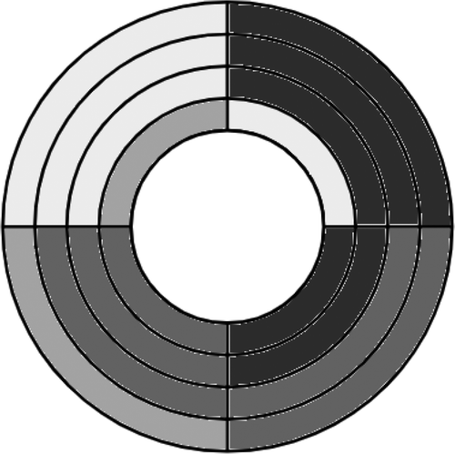
DONUTS instances are composed of two subsets of bar charts. The first subset S1 requires bins (an even number) to be filled and is generated as a TRIPLETS instance. The second subset S2 requires bins (an even number) to be filled if subtours are allowed and bins otherwise and is called a donut. We show in Figure 8 an illustrative example of a donut composed of n = 4 bar charts with , and c = 4. We observe that the optimal 2-BCPP solution for this instance requires five bins but that a solution using four bins can be reached if it is allowed to pack the first item of bar chart 4 in bin 4 (top left in the figure) and the second item in bin 1 (top right in the figure) or, in other words, if Eulerian-flow subtour is not forbidden. In data set DONUTS, subset S2 is generated as a TRIPLETS instance except for j = 1 and . For j = 1, the first item of the first bar chart is in the range , whereas the first item of the second bar chart is in the range . For , the second item of the first bar chart is in the range , whereas the second item of the second bar chart is in the range . An additional bar chart with weights is added to the subset to complete the donut. Note that in order to make sure that a DONUTS instance requires an extra bin when subtours are forbidden, we need to generate the bar charts in S2 so that they cannot be mixed with the bar charts in S1 to build a feasible 2-BCPP solution using bins. We also point out that subset S2 alone is not a valid DONUTS instance because the solution using bins does not contain node (0, 0) (secondary node 0), whereas having a flow going out of (0, 0) (0) is a constraint in EUL-FLOW (LINK-FLOW).
For data set TRIPLETS, we consider three bin capacities and four values for the number of bins (which corresponds to bar charts, respectively). For each of the 12 combinations, we generate 10 instances resulting in 120 instances in total. For data set DONUTS, we considered the same three bin capacities and four values for the number of bins in the first subset . We considered two options for (the number of bins in the second subset): 2 and . We also evaluated the impact of adding three donuts per instance instead of one (i.e., generating three distinct subsets S2). For each of the combinations, we generate 10 instances resulting in 480 instances in total.
5.2.2. Data Set Motivation.
Data set TRIPLETS originates from the well-known “triplets” data set introduced by Falkenauer (1996) for the BPP. These instances are shown to be difficult to solve in practice because there are very few optimal solutions, meaning that a lot of exploration is needed in order to find one of these optimal solutions. Data set DONUTS originates from the “ANI” instances introduced by Delorme et al. (2016) for the BPP. These instances are shown to be difficult to solve in practice because the optimal solution is one bin away from the lower bound derived from the LP relaxation of the existing models, meaning that a lot of exploration is needed in order to prove that a solution with value equal to the lower bound does not exist.
5.2.3. Experiments.
We display in Table 5 the results obtained by each of the tested approaches on data set TRIPLETS.
|
Table 5. Results of the Tested Approaches for TRIPLETS Instances
| CSP | EUL-REL | LINK-REL | ERZIN | EUL-FLOW | LINK-FLOW | 2DV | GA_LO | |||||||||||||||
|---|---|---|---|---|---|---|---|---|---|---|---|---|---|---|---|---|---|---|---|---|---|---|
| c | Avg. opt. value | diff | # opt | time | diff | # opt | time | diff | # opt | time | abs gap | # opt | time | abs gap | # cuts | # opt | time | abs gap | # cuts | diff | diff | |
| 80 | 20 | 20 | 0 | 9 | 0 | 0 | 6 | 0 | 0 | 8 | 1,804 | 0.2 | 10 | 0 | 0 | 2.3 | 10 | 0 | 0 | 0.9 | 3 | 4 |
| 50 | 50 | 0 | 4 | 3 | 0 | 4 | 2 | 0 | 0 | 3,600 | 2.0 | 9 | 366 | 0.1 | 382.6 | 10 | 3 | 0 | 3.6 | 4 | 9 | |
| 100 | 100 | 0 | 5 | 4 | 0 | 5 | 4 | 0 | 0 | 3,600 | 4.0 | 10 | 13 | 0 | 7.8 | 10 | 12 | 0 | 3.3 | 8 | 18 | |
| 250 | 250 | 0 | 6 | 15 | 0 | 7 | 73 | 0 | 0 | 3,600 | 9.4 | 10 | 13 | 0 | 3.2 | 10 | 77 | 0 | 0.6 | 19 | 43 | |
| 240 | 20 | 20 | 0 | 10 | 0 | 0 | 10 | 0 | 0 | 10 | 235 | 0 | 10 | 0 | 0 | 0.9 | 10 | 0 | 0 | 0 | 3 | 4 |
| 50 | 50 | 0 | 2 | 58 | 0 | 0 | 52 | 0 | 0 | 3,600 | 2.0 | 10 | 102 | 0 | 6.4 | 10 | 240 | 0 | 7.7 | 5 | 9 | |
| 100 | 100 | 0 | 5 | 152 | 0 | 4 | 289 | 0 | 0 | 3,600 | 3.8 | 9 | 516 | 0.1 | 101.9 | 8 | 1,019 | 0.2 | 6.4 | 8 | 19 | |
| 250 | 250 | 0 | 5 | 731 | 0 | 3 | 734 | 0 | 0 | 3,600 | 10.7 | 9 | 1,775 | 0.1 | 10.6 | 9 | 1,262 | 0.2 | 3.8 | 18 | 43 | |
| 400 | 20 | 20 | 0 | 10 | 0 | 0 | 10 | 0 | 0 | 9 | 383 | 0.1 | 10 | 0 | 0 | 0.3 | 10 | 0 | 0 | 0.2 | 3 | 4 |
| 50 | 50 | 0 | 9 | 21 | 0 | 10 | 15 | 0 | 0 | 3,600 | 2.1 | 10 | 31 | 0 | 7.8 | 10 | 13 | 0 | 0.2 | 5 | 10 | |
| 100 | 100 | 0 | 0 | 3,300 | 0 | 0 | 3,600 | 0 | 0 | 3,600 | 3.9 | 1 | 3,475 | 0.9 | 4.7 | 0 | 3,600 | 1.0 | 0.9 | 8 | 19 | |
| 250 | 250 | 0 | 1 | 3,583 | 0 | 0 | 3,600 | 0 | 0 | 3,600 | 11.2 | 0 | 3,600 | 1.3 | 2.8 | 1 | 3,561 | 0.9 | 3 | 20 | 46 | |
We observe that the lower bounds derived from CSP, EUL-REL, and LINK-REL are always equal to the optimal solution value, which does not come as a surprise as every TRIPLETS instance has an optimal solution that does not contain any loss space. Regarding upper bounding procedures, we notice that GA_LO does not perform particularly well. This can be explained by the remarkable structure of TRIPLETS instances in which a bin becomes unusable as soon as it is filled above the threshold , which is a property that GA_LO does not take into account. ERZIN is only able to solve instances with to optimality (i.e., with 29 bar charts). Further analysis available in Online Table 11 shows that such bad performance can be attributed to neither the model size (which is comparable to the size of EUL-FLOW and LINK-FLOW) nor the quality of the LP-relaxation bound (which is always equal to the optimal solution value). A possible explanation could be that the solutions obtained after solving a node in the branch-and-bound tree are rarely integer and these solutions do not allow Gurobi heuristics to find good quality upper bounds. EUL-FLOW and LINK-FLOW are able to solve most instances except the largest ones (when c = 400 and or ). Neither approach is clearly better than the other. As previously mentioned, a reason could be that EUL-FLOW structure makes it easier for Gurobi heuristics to find good quality solutions even though LINK-FLOW models are smaller. Finally, we note that the number of cuts required by EUL-FLOW varies a lot (between 0 and 3,702) compared with the number of cuts required by LINK-FLOW (between 0 and 38).
We show in Table 6 the results obtained by each of the tested approaches on data set DONUTS grouped by the bin capacity c and the number of bins in the first subset . The lower bounds derived from CSP, EUL-REL, and LINK-REL are now always one bin away from the optimal solution value, which is expected as DONUTS instances were made with that purpose. We note that GA_LO is still outperformed by 2DV (as far as upper bound quality is concerned) and that ERZIN still displays poor performance compared with the other models. LINK-FLOW is able to solve all but 15 instances and is clearly better than EUL-FLOW. This is due to smaller models (see Online Table 12) and a reduced number of required cuts. Further analysis is reported in Table 7 in which the results for the data set are grouped by number of donuts (column “# don”) and number of bins per donut (column “”).
|
Table 6. Results of the Tested Approaches for DONUTS Instances Grouped by c and
| CSP | EUL-REL | LINK-REL | ERZIN | EUL-FLOW | LINK-FLOW | 2DV | GA_LO | |||||||||||||||
|---|---|---|---|---|---|---|---|---|---|---|---|---|---|---|---|---|---|---|---|---|---|---|
| c | Avg. opt. value | diff | # opt | time | diff | # opt | time | diff | # opt | time | abs gap | # opt | time | abs gap | # cuts | # opt | time | abs gap | # cuts | diff | diff | |
| 80 | 20 | 27 | 1 | 0 | 0 | 1 | 0 | 0 | 1 | 6 | 3,259 | 0.9 | 40 | 0 | 0 | 15.2 | 40 | 0 | 0 | 3.4 | 1 | 3 |
| 50 | 63 | 1 | 0 | 0 | 1 | 0 | 0 | 1 | 0 | 3,600 | 2.1 | 37 | 374 | 0.1 | 3,210.4 | 40 | 0 | 0 | 3.3 | 4 | 9 | |
| 100 | 123 | 1 | 0 | 0 | 1 | 0 | 0 | 1 | 0 | 3,600 | 3.7 | 40 | 24 | 0 | 1,236.3 | 40 | 1 | 0 | 1.9 | 7 | 17 | |
| 250 | 303 | 1 | 0 | 0 | 1 | 0 | 0 | 1 | 0 | 3,600 | 8.4 | 39 | 149 | 0 | 3,409.8 | 40 | 1 | 0 | 1.7 | 18 | 44 | |
| 240 | 20 | 27 | 1 | 0 | 0 | 1 | 0 | 0 | 1 | 0 | 3,600 | 1.1 | 40 | 2 | 0 | 7.1 | 40 | 0 | 0 | 2.8 | 2 | 4 |
| 50 | 63 | 1 | 0 | 4 | 1 | 0 | 3 | 1 | 0 | 3,600 | 2.6 | 31 | 817 | 0.2 | 1,812.9 | 40 | 7 | 0 | 24.7 | 5 | 10 | |
| 100 | 123 | 1 | 0 | 13 | 1 | 0 | 9 | 1 | 0 | 3,600 | 5.0 | 30 | 911 | 0.2 | 1,635.5 | 40 | 34 | 0 | 5.1 | 8 | 20 | |
| 250 | 303 | 1 | 0 | 52 | 1 | 0 | 41 | 1 | 0 | 3,600 | 13.5 | 20 | 1,810 | 0.6 | 2,914.2 | 39 | 337 | 0 | 3.5 | 20 | 51 | |
| 400 | 20 | 27 | 1 | 0 | 1 | 1 | 0 | 0 | 1 | 2 | 3,520 | 1.1 | 40 | 2 | 0 | 6.3 | 40 | 0 | 0 | 2.1 | 2 | 4 |
| 50 | 63 | 1 | 0 | 11 | 1 | 0 | 7 | 1 | 0 | 3,600 | 2.6 | 39 | 125 | 0 | 16.1 | 40 | 11 | 0 | 6.2 | 4 | 10 | |
| 100 | 123 | 1 | 0 | 93 | 1 | 0 | 47 | 1 | 0 | 3,600 | 5.2 | 30 | 968 | 0.2 | 936.3 | 36 | 522 | 0.1 | 78.9 | 9 | 21 | |
| 250 | 303 | 1 | 0 | 391 | 1 | 0 | 267 | 1 | 0 | 3,600 | 17.0 | 20 | 1,849 | 0.6 | 1,227.6 | 30 | 1,511 | 0.3 | 114.5 | 21 | 52 | |
|
Table 7. Results of the Tested Approaches for DONUTS Instances Grouped by the Number of Donuts and
| CSP | EUL-REL | LINK-REL | ERZIN | EUL-FLOW | LINK-FLOW | 2DV | GA_LO | |||||||||||||||
|---|---|---|---|---|---|---|---|---|---|---|---|---|---|---|---|---|---|---|---|---|---|---|
| # don | Avg. opt. value | diff | # opt | time | diff | # opt | time | diff | # opt | time | abs gap | # opt | time | abs gap | # cuts | # opt | time | abs gap | # cuts | diff | diff | |
| 1 | 2 | 108 | 1 | 0 | 5 | 1 | 0 | 10 | 1 | 8 | 3,460 | 3.4 | 120 | 13 | 0 | 2,379.3 | 120 | 52 | 0 | 38.8 | 7 | 17 |
| 1 | 0.2 | 127 | 1 | 0 | 46 | 1 | 0 | 32 | 1 | 0 | 3,600 | 5.0 | 99 | 670 | 0.2 | 2.8 | 111 | 314 | 0.1 | 2.4 | 9 | 20 |
| 3 | 2 | 112 | 1 | 0 | 9 | 1 | 0 | 12 | 1 | 0 | 3,600 | 3.9 | 120 | 19 | 0 | 3,088.9 | 120 | 61 | 0 | 38.1 | 7 | 18 |
| 3 | 0.2 | 169 | 1 | 0 | 129 | 1 | 0 | 69 | 1 | 0 | 3,600 | 8.8 | 67 | 1,641 | 0.4 | 4.9 | 114 | 382 | 0 | 3.4 | 10 | 26 |
We observe that instances with large donuts (when ) are much harder to solve than instances with small donuts (when ). This can be explained by two reasons: (i) instances with large donuts contain more bar charts and, thus, result in larger models, and (ii) instances with large donuts require more cuts to be solved to optimality than instances with small donuts, especially for EUL-FLOW. We also notice that instances with three donuts require more time to be solved on average than instances with one donut.
6. Conclusions and Future Research
We study the 2-BCPP, a combinatorial optimization problem introduced recently by Erzin et al. (2021b) that is particularly interesting as it lies at the intersection of many well-known packing problems. We start by clustering relevant packing problems into three groups (those that are 2-BCPP relaxations, those for which the 2-BCPP is a relaxation, and those for which the 2-BCPP is a special case) and showing how solving these problems can provide a lower bound, an upper bound, or an optimal solution to the 2-BCPP. We then introduce two new ILP models based on the arcflow formulation in which a 2-BCPP solution is represented as one or several cycles in a graph in which nodes are partial bin fillings: Eulerian-flow and link-flow. The former model represents a solution as a single Eulerian cycle, whereas the latter model represents a solution as a set of cycles that complete each other. Even though both models require an exponential number of subtour elimination constraints, we show that these constraints can initially be omitted and added on the fly within a constraint generation framework. We create six data sets to test our approaches: four inspired by the 2-BCPP literature in which the bar chart weights are uniformly distributed and two inspired by the bin packing literature that were designed to be very hard to solve because either the upper bound is difficult to reach or the lower bound is difficult to raise. Even though we empirically show that our new algorithms clearly obtain better performance than the only exact approach proposed in the literature, we also identify instance features for which our methods did not perform very well because of a very large number of variables and constraints involved. Such features are (i) a large bin capacity and (ii) a large number of distinct small bar charts. Overall, we show that our exact approaches can easily solve instances with up to 1,000 bar charts when the bin capacity is limited to 100 and instances with up to 100 bar charts when the bin capacity is limited to 500, which is a huge improvement with respect to the literature. We also show that the performance of the existing 2-BCPP model does not depend on the same instance features as our new models (K and n for the former, c and n for the latter).
Even though our exact approaches obtain state-of-the-art results for the 2-BCPP, we should keep in mind that the problem does not have many practical applications because of the constraint limiting the number of items in a bar chart to two. Nevertheless, it is the first time (to the best of our knowledge) that an arcflow model is proposed for a bin packing problem with a form of precedence constraints, which indicates that our approaches can be extended to solve other packing problems with precedence constraints. It is also the first time that an arcflow model is solved within a constraint generation framework. This means that such formulations can be used in decomposition approaches in which the master problem is a packing problem (e.g., the Benders’ decomposition approach of Côté et al. 2021 for the two-dimensional bin packing problem) instead of Kantorovich-like models that are known to have a very poor LP-relaxation value. As far as the generalization of our approaches to the n-BCPP is concerned, it would be interesting to see the computational behavior of Eulerian-flow and link-flow extensions for the 3-BCPP. We expect them to work well for small bin capacities (up to 100 if the instance is composed of few bar charts or up to 50 otherwise). It would also be interesting to study similar extensions for the 4-BCPP and 5-BCPP. There, we expect that the full graph cannot be generated anymore and alternative strategies are required. A first option could be to only add the arcs that are likely to be selected in an optimal solution (e.g., by using rules of thumb or machine learning techniques), which would result in a matheuristic. A second option could be to generate the arcs with column generation and embed the approach in a branch-and-price algorithm.
We thank the two anonymous reviewers for their valuable comments that helped to improve the presentation of this paper.
1 Indeed, link https://disk.yandex.ru/d/U-EK0n4Z_HEAeQ states that the solution found by CPLEX for the first instance of “class N = 10” is 10, whereas all our models indicate that the optimal solution is 12.
References
- (2016) Bin packing and related problems: General arc-flow formulation with graph compression. Comput. Oper. Res. 69:56–67.Crossref, Google Scholar
- (2019) Reinforcement learning driven heuristic optimization. Preprint, submitted June 16, https://arxiv.org/abs/1906.06639.Google Scholar
- (2013)
Bin packing approximation algorithms: Survey and classification . Pardalos P, Du DZ, Graham R, eds. Handbook of Combinatorial Optimization (Springer, New York).Crossref, Google Scholar - (2018) The meet-in-the-middle principle for cutting and packing problems. INFORMS J. Comput. 30(4):646–661.Link, Google Scholar
- (2014) Combinatorial Benders’ cuts for the strip packing problem. Oper. Res. 62(3):643–661.Link, Google Scholar
- (2021) Combinatorial Benders decomposition for the two-dimensional bin packing problem. INFORMS J. Comput. 33(3):963–978.Link, Google Scholar
- (2022) Arc flow formulations based on dynamic programming: Theoretical foundations and applications. Eur. J. Oper. Res. 296(1):3–21.Crossref, Google Scholar
- (2012) The bin packing problem with precedence constraints. Oper. Res. 60(6):1491–1504.Link, Google Scholar
- (2019) Mathematical models and decomposition methods for the multiple knapsack problem. Eur. J. Oper. Res. 274(3):886–899.Crossref, Google Scholar
- (2020) Enhanced pseudo-polynomial formulations for bin packing and cutting stock problems. INFORMS J. Comput. 32(1):101–119.Link, Google Scholar
- (2016) Bin packing and cutting stock problems: Mathematical models and exact algorithms. Eur. J. Oper. Res. 255(1):1–20.Crossref, Google Scholar
- (2017) Logic based Benders’ decomposition for orthogonal stock cutting problems. Comput. Oper. Res. 78:290–298.Crossref, Google Scholar
- (2021) Solution methods for scheduling problems with sequence-dependent deterioration and maintenance events. Eur. J. Oper. Res. 295(3):823–837.Crossref, Google Scholar
- (2021a) A posteriori analysis of the algorithms for two-bar charts packing problem. Olenev NN, Evtushenko YG, Malkova V, Jacimovic M, Khachay M, eds. Advances in Optimization and Applications, vol. 1514, Communications in Computer and Information Science Series (Springer, Cham, Switzerland), 201–216.Google Scholar
- (2021b) Two-bar charts packing problem. Optim. Lett. 15(6):1955–1971.Crossref, Google Scholar
- (2021c) A 3/2-approximation for big two-bar charts packing. J. Combin. Optim. 42(1):71–84.Crossref, Google Scholar
- (1996) A hybrid grouping genetic algorithm for bin packing. J. Heuristics 2(1):5–30.Crossref, Google Scholar
- (1960) Mathematical methods of organizing and planning production. Management Sci. 6(4):366–422.Link, Google Scholar
- (2022) Bin packing problem with time lags. INFORMS J. Comput. 34(4):2249–2270.Link, Google Scholar
- (2004) A new branch-and-cut algorithm for the capacitated vehicle routing problem. Math. Programming 100(2):423–445.Crossref, Google Scholar
- (2010) Arc-flow model for the two-dimensional guillotine cutting stock problem. Comput. Oper. Res. 37(6):991–1001.Crossref, Google Scholar
- (1990) Knapsack Problems: Algorithms and Computer Implementations (John Wiley & Sons, Chichester, UK).Google Scholar
- (2003) An exact approach to the strip-packing problem. INFORMS J. Comput. 15(3):310–319.Link, Google Scholar
- (2016) Integer linear programming models for the skiving stock problem. Eur. J. Oper. Res. 251(2):356–368.Crossref, Google Scholar
- (2010) Algorithms for the bin packing problem with conflicts. INFORMS J. Comput. 22(3):401–415.Link, Google Scholar
- (2018) Mathematical models and decomposition algorithms for makespan minimization in plastic rolls production. J. Oper. Res. Soc. 69(3):326–339.Crossref, Google Scholar
- (2016) Procedures for the bin packing problem with precedence constraints. Eur. J. Oper. Res. 250(3):794–806.Crossref, Google Scholar
- (2020) A generic exact solver for vehicle routing and related problems. Math. Programming 183(1):483–523.Crossref, Google Scholar
- (2017) Generating subtour elimination constraints for the TSP from pure integer solutions. Central Eur. J. Oper. Res. 25(1):231–260.Crossref, Google Scholar
- (2013) Bin packing with conflicts: A generic branch-and-price algorithm. INFORMS J. Comput. 25(2):244–255.Link, Google Scholar
- (2004)
A constraint for bin packing . Wallace M, ed. Principles and Practice of Constraint Programming—CP 2004, Lecture Notes in Computer Science, vol. 3258 (Springer, Berlin, Heidelberg), 648–662.Crossref, Google Scholar - (1990) A one-dimensional cutting stock problem in the aluminium industry and its solution. Eur. J. Oper. Res. 44(2):209–223.Crossref, Google Scholar
- (1999) Exact solution of bin-packing problems using column generation and branch-and-bound. Ann. Oper. Res. 86:629–659.Crossref, Google Scholar
- (1998) Branch-and-price algorithms for the one-dimensional cutting stock problem. Comput. Optim. Appl. 9(3):211–228.Crossref, Google Scholar
- (2020a) A branch-and-price algorithm for the two-dimensional vector packing problem. Eur. J. Oper. Res. 281(1):25–35.Crossref, Google Scholar
- (2020b) A new branch-and-price-and-cut algorithm for one-dimensional bin-packing problems. INFORMS J. Comput. 32(2):428–443.Link, Google Scholar
- (1977) Valid inequalities, covering problems and discrete dynamic programs. Hammer PL, Johnson EL, Korte BH, Nemhauser GL, eds. Studies in Integer Programming, vol. 1, Annals of Discrete Mathematics (Elsevier), 527–538.Google Scholar

