Learning-Based Online Optimization for Autonomous Mobility-on-Demand Fleet Control
Abstract
Autonomous mobility-on-demand systems are a viable alternative to mitigate many transportation-related externalities in cities, such as rising vehicle volumes in urban areas and transportation-related pollution. However, the success of these systems heavily depends on efficient and effective fleet control strategies. In this context, we study online control algorithms for autonomous mobility-on-demand systems and develop a novel hybrid combinatorial optimization-enriched machine learning pipeline which learns online dispatching and rebalancing policies from optimal full-information solutions. We test our hybrid pipeline on large-scale real-world scenarios with different vehicle fleet sizes and various request densities. We show that our pipeline outperforms greedy and model-predictive control approaches with respect to various key performance indicators (KPIs), for example, by up to 17.1% and on average by 6.3% in terms of realized profit, and on average by 4.7% in terms of satisfied customers.
History: Accepted by Andrea Lodi, Area Editor for Design & Analysis of Algorithms–Discrete.
Funding: This work was supported by Deutsche Forschungsgemeinschaft [Grant 449261765].
Supplemental Material: The software that supports the findings of this study is available within the paper and its Supplemental Information (https://pubsonline.informs.org/doi/suppl/10.1287/ijoc.2024.0637) as well as from the IJOC GitHub software repository (https://github.com/INFORMSJoC/2024.0637). The complete IJOC Software and Data Repository is available at https://informsjoc.github.io/.
1. Introduction
Growing urbanization leads to rising traffic volumes in urban areas and challenges the sustainability and economic efficiency of today’s urban transportation systems. In fact, transportation systems’ externalities, such as congestion and local emissions, can significantly damage public health and pose a growing threat to our environment (Levy et al. 2010, Schrank et al. 2019). Moreover, private cars currently require considerable space for parking and driving in urban areas.
Recent progress in autonomous driving and 5G technology has led to crucial advances toward enabling autonomous mobility-on-demand (AMoD) systems (White 2020), which can contribute to mitigating many of the aforementioned challenges in the coming years. An AMoD system consists of a centrally controlled fleet of self-driving vehicles serving on-demand ride requests (Pavone 2015). To manage the fleet, a central controller dispatches ride requests to vehicles in order to transport customers between their origin and destination. The central controller may further relocate idle vehicles to better match future demand, for example, in high-demand areas. An AMoD system has many advantages over current conventional ride-hailing systems. Among others, it permits centralized control and therefore enables system-optimal dispatching decisions. Moreover, it allows for a high utilization of vehicles which results from rebalancing actions. However, the utilization of an AMoD system depends on its efficient operation, that is, system-optimal online dispatching and rebalancing of the vehicle fleet. Designing such an efficient control algorithm for AMoD systems faces two major challenges. First, the underlying planning problem is an online control problem; that is, the central controller must take dispatching and rebalancing decisions under uncertainty without knowing future ride requests. Second, the scalability of the control mechanism for large-scale applications can be computationally challenging as dozens of thousands of requests will need to be satisfied every hour in densely populated areas.
Against this background, we develop a novel family of scalable online control policies that receive an online AMoD system state as input and return dispatching and rebalancing actions for the AMoD fleet. Specifically, we encode these online control policies via a hybrid combinatorial optimization (CO)-enriched machine learning (ML) pipeline. The rationale of this hybrid CO-enriched ML pipeline is to transform the online AMoD system state into a combinatorial dispatching problem, and to learn the parameterization of this dispatching problem from optimal full-information solutions, based on historical data. As a result, the solution of the dispatching problem imitates optimal full-information solutions and leads to anticipative online dispatching and rebalancing actions.
1.1. Related Work
Our work contributes to two different research streams. From an application perspective, it connects to vehicle routing and dispatching problems for AMoD systems. From a methodological perspective, it connects to the field of CO-enriched ML. In this section, we first review related works in the field of AMoD systems and refer to Vidal et al. (2020) for a general overview of vehicle routing problems. Second, we review related works at the intersection of ML and CO, and refer to Bengio et al. (2021) and Kotary et al. (2021) for a general overview.
1.1.1. AMoD Systems.
AMoD systems have been studied from a system perspective and from an operational perspective. Studies that focused on the system perspective investigated offline problem settings with full information on all ride requests, addressing research questions related to strategic decision making and mesoscopic analyses, and are only loosely related to our work. Therefore, we exclude these from our review and refer to Zardini et al. (2022) for a general overview.
This study relates to the operational perspective, specifically to online systems with ride requests entering the system sequentially over time. To solve such an online dispatching problem, classical CO approaches which leverage the combinatorial structure of the problem, as well as ML approaches which learn to account for the uncertain appearance of future ride requests, exist. In the context of classical CO, Bertsimas et al. (2019) introduced an online reoptimization algorithm, which iteratively optimizes the dispatching of available vehicles to new ride requests when they enter the system in a rolling horizon fashion. Other works focused explicitly on relocating unassigned vehicles to areas of high future demand to reduce waiting times for future ride requests (Pavone et al. 2012, Zhang and Pavone 2016, Iglesias et al. 2018, Liu and Samaranayake 2022). As the efficiency of dispatching and rebalancing depends on future ride requests, model-predictive control (Alonso-Mora et al. 2017) and stochastic model-predictive control algorithms (Tsao et al. 2018) have been developed to incorporate information about future ride requests. A complementary stream of research studied similar problems from a deep reinforcement learning (DRL) perspective, explicitly focusing on rebalancing (Gammelli et al. 2021, Jiao et al. 2021, Liang et al. 2022, Skordilis et al. 2022) or nonmyopic (anticipative) dispatching (Xu et al. 2018, Li et al. 2019, Tang et al. 2019, Zhou et al. 2019, Sadeghi Eshkevari et al. 2022, Enders et al. 2023).
As can be seen, nonmyopic dispatching and rebalancing for AMoD systems have recently been vividly studied. Existing approaches either follow a DRL paradigm to account for uncertain system dynamics or focus on classical optimization-based (control) approaches that are often extended by a sequential prediction component. However, a truly integrated approach that aims to combine learning and optimization to leverage the advantages of both concepts simultaneously has not been studied so far.
1.1.2. Combinatorial Optimization-Enriched Machine Learning.
In many applications, combinatorial decisions are subject to uncertainty. In this context, various approaches that enrich CO by ML components to account for uncertainty have recently been studied. For example, Donti et al. (2017) proposed an end-to-end learning approach for probabilistic models in the course of stochastic optimization, and Elmachtoub and Grigas (2022) introduced a loss to learn a prediction model for travel times by utilizing the structure of the underlying vehicle routing problem. Closest to our paradigm are approaches which we can generally refer to as CO-enriched ML pipelines (cf. Dalle et al. 2022). In particular, these approaches revolve around the concept of structured learning (SL), a supervised learning methodology with a combinatorial solution space (cf. Nowozin and Lampert 2011), which can be used to enrich CO algorithms with a prediction component. Parmentier (2021) used SL to parameterize a computationally tractable surrogate problem such that its solution approximates the solution of a hard combinatorial problem. Using this concept, Parmentier and T’Kindt (2023) solved a single-machine scheduling problem with release dates by transforming it into a computationally tractable scheduling problem without release dates.
These recent works point toward the efficiency of CO-enriched ML when determining approximate solutions for hard-to-solve combinatorial problems. However, it remains an open question whether CO-enriched ML can also successfully be used to derive efficient online control policies, especially in the realm of AMoD systems.
1.2. Contributions
In this paper, we introduce a new family of scalable online control policies for large-scale online dispatching and rebalancing of AMoD systems. To reach this goal, we close the research gaps outlined above by introducing a novel family of online control policies, encoded via a hybrid CO-enriched ML pipeline. In a nutshell, this hybrid CO-enriched ML pipeline receives an AMoD system state, transforms it into a combinatorial dispatching problem, parameterizes the dispatching problem by utilizing SL, and solves it to return online dispatching and rebalancing actions. The main rationale of this hybrid CO-enriched ML pipeline is to learn the parameterization of the dispatching problem from optimal full-information solutions for historical data, in such a way that the resulting policy imitates fully informed dispatching and rebalancing actions.
The contribution of our work is several-fold. First, we present a novel CO-enriched ML pipeline, amenable to derive online control policies, and tailor it to online dispatching and rebalancing for AMoD systems. Second, to establish this pipeline, we show how to solve the underlying CO problem, namely, a dispatching and rebalancing problem, in polynomial time. Third, we show how to learn a parameterization for the underlying CO problem based on optimal full-information solutions from historical data using an SL approach. Fourth, we derive two online control policies, namely, a sample-based (SB) approach and a cell-based (CB) approach, both utilizing our hybrid CO-enriched ML pipeline. Fifth, we present a numerical study based on real-world data to benchmark the encoded policies against a greedy policy and a sampling-based receding horizon approach (cf. Alonso-Mora et al. 2017).
Our results show that our learning-based policies outperform a greedy policy with respect to realized profit by up to 17.1% and by 6.3% on average. Moreover, our learning-based policies robustly perform better than a greedy policy across various scenarios, whereas a sampling-based policy oftentimes performs worse than the greedy policy. In general, a sampling-based policy shows an inferior performance compared with our learning-based policies, even in the scenarios where it improves upon the greedy policy. Finally, we show that our learning-based policies yield a good trade-off between anticorrelated key performance indicators (KPIs); for example, when maximizing the total profit or the number of served customers, we still obtain a lower distance driven per vehicle compared with policies that show worse performance on the aforementioned quantities.
1.3. Organization
The remainder of this paper is structured as follows. In Section 2, we detail our problem setting. In Section 3, we introduce our hybrid CO-enriched ML pipeline and derive the SL problem to learn an ML predictor which parameterizes the underlying CO problem. We present a real-world case study in Section 4 and its numerical results in Section 5. Section 6 finally concludes the paper.
2. Problem Setting
We study an online vehicle routing problem from the perspective of an AMoD system’s central controller, which steers a homogeneous fleet of self-driving vehicles. The central controller either dispatches vehicles to serve ride requests or rebalances idle vehicles to anticipate future ride requests. Here, a ride request can represent a solitary ride or pooled rides, as we assume decisions on pooling requests to be taken at an upper planning level. Accordingly, each ride request demands a mobility service from an origin to a destination location at a certain point in time. The central controller takes decisions according to a discrete time horizon . We denote the period between the actual decision time t and the subsequent decision time t + 1 as system time period . We consider a set of vehicles that serve requests. Each ride request is a quintuple with a pick-up location or, a drop-off location dr, a start time sr, an arrival time ar, and its reward pr. Here, the start time sr and the arrival time ar are the times when the vehicle reaches the origin or and destination dr of the ride request, respectively. Let denote the driving time of a vehicle between two locations l1 and l2. The start time sr, the arrival time ar, and the driving time are not subject to the time discretization but are from a continuous time range in . If the central controller assigns a ride request to a vehicle, the vehicle has to fulfill this ride request. We refer to a sequence of ride requests that a vehicle fulfills as a trip.
2.1. System State
At any decision time t, the state of a vehicle v is a pair composed of its current location and a sequence of unfinished requests. A request r is unfinished when . The sequence is empty when the vehicle has already fulfilled all assigned requests, which means that the vehicle is idling. Regarding the overall AMoD system state, the state comprises the batch Rt of requests that entered the system between the previous decision time t − 1 and t with , as well as the state of each vehicle . Note that requests with a starting time are known to the central controller at decision time t.
2.2. Feasible Decisions
Given the current state of the system xt, the central controller determines at decision time t which requests to accept and assigns them to vehicles. The central controller can also rebalance a vehicle after the last request in its trip or when it is idling. A feasible decision for vehicle v given its current state is a trip, that is, a sequence of requests . Here, is the updated trip , which includes unfinished requests from that were already assigned to v at previous decision times, and new requests from batch Rt. Additionally, may include a final rebalancing location l. As we solve an online decision-making problem, trip sequences are usually short; that is, they contain no more than one request from previous decision times, a newly assigned request, and possibly a rebalancing location. Still, our definition of a trip permits a significantly longer request sequence, in such a way that we can later on use the online problem statement to also characterize the respective offline full-information planning problem by considering only a single time step that spans the whole planning horizon.
We denote the central controller decision with set yt comprising all vehicle-specific decisions, The central controller’s decision needs to satisfy the following constraints:
Each request in a trip of vehicle v does not belong to a trip of another vehicle , formally . Note that two trips can have the same rebalancing location.
For every pair of successive requests, the respective vehicle can reach the origin of on time after ri, that is, .
If the first request r1 in a trip of vehicle v is new, that is, , then it must be reachable from the current location of the vehicle: .
We denote with the set of feasible operator decisions for system state xt.
2.3. Evolution of the System
Once the central controller dispatches the decision yt from decision time t, the system evolves until t + 1. Each vehicle v drives along its trip. If a vehicle completes its trip before t + 1, it idles. If the vehicle does not reach its rebalancing location l before t + 1, it starts idling at t + 1 and awaits the next operator’s decision. We can therefore deduce from its position at t + 1. The system removes all requests from Rt that were assigned at time t. Furthermore, requests from Rt which remained unassigned at t leave the system. New requests enter the system between t and t + 1.
2.4. Policy
Let denote the set of possible AMoD system states. A (deterministic) policy is a mapping that assigns to any AMoD system state x a decision .
2.5. Objective
Let us denote by the reward made by vehicle v at time t. The reward at time t is therefore
We may adjust the objective by changing the interpretation of ; for example, we can maximize the total profit by accounting for trip-dependent rewards and costs. Alternatively, we can maximize the number of served requests by setting to the number of requests that vehicle v serves at time t. Our objective is to find a policy δ that maximizes the total reward over all vehicle trips at the end of the problem time horizon T,
2.6. Full-Information Upper Bound
To keep the paper concise, we reuse the online problem setting to further define its respective offline full-information counterpart. To do so, we keep the length of the considered time horizon but remove its discretization such that all requests are already in the system at time t = 1. By doing so, we obtain full information of all requests and the solution that we obtain by solving this single (but large) time step equals the solution of the respective offline decision-making problem. Although establishing this equivalence may appear cumbersome at this point, it will allow us to devise one polynomial algorithm that is able to solve both the offline and the online problems in the following section.
2.7. Scope and Limitations of the Model
A few comments on this modeling approach are in order. First, we do not permit late arrivals at pick-up locations. When a request enters the system, the central controller decides to either fulfill or reject this request. This assumption aligns with real-world practice: customers typically can choose between various mobility providers such that an unfulfilled request usually leads to a customer choosing another provider’s service or resubmitting the request a bit later. Consequently, operators aim to take immediate action to provide direct feedback to customers. Notably, it is possible to adapt our setting for delayed pick-ups by including unfulfilled requests in the request batch that enters the system in the next system time period. Second, we assume that ride-pooling decisions occur at an upper planning stage. Analyzing whether a hierarchical or an integrated ride-pooling approach is superior for CO-enriched ML online control of AMoD systems remains an open research question for future work. Third, we consider travel time uncertainty on a lower operational level. We can express time uncertainty on the duration of each ride request which has no impact on the presented model.
3. CO-Enriched ML Pipeline
In this section, we propose a CO-enriched ML pipeline that encodes a dispatching and rebalancing policy δ. This pipeline maps an AMoD system state xt to a feasible dispatching and rebalancing decision yt. The main rationale of our pipeline is to combine an ML component with a CO component such that the ML component informs the CO component. Specifically, we use the ML component to parameterize the problem instance solved by the CO component in such a way that the solution generated via the CO component maps to a performant dispatching and rebalancing decision. We will train the statistical model of the ML component in an end-to-end learning fashion, utilizing an imitation-learning paradigm that utilizes the information from full-information offline solutions computed on historical data.
Establishing such an algorithmic pipeline is anything but trivial and requires several building blocks detailed in the following subsections. In Section 3.1, we first introduce a polynomial algorithm that allows us to solve both the full-information offline problem as well as the online problem used in our CO component. This algorithm encodes some feasibility constraints of the planning problem in a specific graph structure, which is essential for our pipeline. After explaining this fundamental basis, we detail the architecture of our algorithmic pipeline in Section 3.2. We continue in Section 3.3 by introducing two slightly different pipelines that allow for rebalancing actions. Both pipelines require mild modifications to the generation of the problem-specific graph structure and differ with respect to their modeling of rebalancing options. Then, we present in Section 3.4 the mechanism to decode the CO solution into dispatching and rebalancing actions. In Section 3.5, we introduce the ML component. Finally, we elaborate on our learning paradigm in Section 3.6.
3.1. Dispatching Problem
In the following, we introduce a polynomial algorithm that allows us to solve the vehicle-to-request dispatching problem as detailed in Section 2. To ease the exposition of this algorithm, we will for now ignore rebalancing decisions and focus on the full-information problem variant. We will then elaborate on how to incorporate rebalancing decisions for online decision making into this algorithm in Section 3.3.
The main idea of our polynomial algorithm is to encode the feasibility constraints of the underlying dispatching problem in a problem-specific graph structure. This will allow us to obtain a solution to the dispatching problem by solving a shortest-path problem on the respective graph. Specifically, we define a dispatching graph as illustrated in Figure 1(a). We construct our dispatching graph as a weighted and directed graph with a set of vertices V, a set of arcs A, and a vector of weights θ, which comprises a weight θa for each arc . To construct this dispatching graph, we proceed as follows.
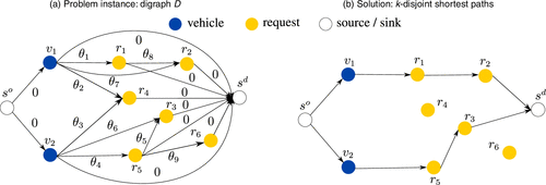
3.1.1. Vertex Set Construction.
The vertex set consists of a vehicle vertex subset, a request vertex subset, a dummy source vertex , and a dummy sink vertex .
Vehicle vertices : For each vehicle in the system, we create a vertex that is related to a specific vehicle and its initial position at the beginning of the time horizon.
Request vertices : For each request that appears in the system during the planning time horizon, we create a vertex that is related to a specific request, its origin-destination pair, and its start time.
3.1.2. Arc Set Construction.
Using the vertex sets as introduced above, we aim to construct the arc set of D such that it encodes the feasibility constraints detailed in Section 2. To do so, we construct A as follows:
We create an arc between two request vertices if Constraint (ii) from Section 2 holds. In this case, we can ensure request-to-request connectivity; that is, the request related to rj can be served after the request related to ri by one and the same vehicle.
We create an arc between a vehicle vertex and a request vertex if Constraint (iii) from Section 2 holds. In this case, we can ensure vehicle-to-request connectivity; that is, when starting at its initial position, the vehicle related to vertex vi can serve the request related to vertex vj.
Finally, we connect the dummy source vertex with each vehicle vertex, and connect all vehicle, request, and artificial vertices to the dummy sink.
Following this vertex and arc construction, we obtain a dispatching graph that represents the constraints detailed in Section 2. We will now continue to explain how a solution to the dispatching problem of Section 2 can be modeled in D to finally show how such a solution can be computed efficiently.
3.1.3. Solution Encoding.
First, we recall that a feasible decision is a set of feasible and disjoint vehicle trips . Next, we observe that our dispatching graph D is acyclic by construction. Then, a path in D that starts at the dummy source vertex and ends at the dummy sink vertex represents a feasible vehicle trip. This trip can unambiguously be associated with a vehicle as its second vertex is always a vehicle vertex.
3.1.4. Algorithm.
To finally devise our algorithm, we assign a weight θa to each arc . We set the weights of arcs that enter the sink or leave the source to zero. Additionally, we set the weights of arcs that enter a request vertex according to the associated negative reward to service this request. We can then find an optimal solution to our vehicle-to-request dispatching problem that maximizes the total reward of the central controller by solving a k-disjoint shortest-paths problem (k-dSPP) on , with k being the number of vehicles of the AMoD fleet. Figure 1(b) illustrates an example of a resulting solution in which each disjoint path defines a trip sequence for a specific vehicle. Recall that the resulting solution is feasible as the disjointness of the paths ensures Constraint (i), whereas Constraints (ii)–(iii) are ensured because of the structure of . The complexity of solving a k-dSPP on is in (cf. Schiffer et al. 2021), such that we obtain a polynomial algorithm to solve the problem of dispatching vehicles to requests.
3.1.5. Discussion.
Although we introduced the polynomial algorithm outlined above for the full-information setting, it can also be applied to solve a respective online decision-making problem. In this case, the only changes that need to be made are (i) limiting the construction of request vertices to requests that are available during the respective system time period, and (ii) associating each vehicle vertex no longer with its initial location but with its respective location upon finishing its last or ongoing trip. Accordingly, the presented algorithm does not only allow us to compute large-scale offline solutions efficiently but further yields an (rebalancing-agnostic) algorithmic skeleton for our online decision-making problem. To finally use this algorithm on our algorithmic pipeline, we will elaborate in Section 3.3 how to integrate rebalancing into the algorithm by modifying the respective dispatching graph.
Three additional comments on our algorithm are in order. First, the resulting solution can contain empty trip sequences that indicate inactive vehicles if this benefits the overall reward maximization. In this case, some paths consist of a vehicle vertex being directly connected to the source and sink vertex. Second, one may change the objective of the central controller by modifying the graph’s weights; for example, to maximize the profit of the central controller, we correct a request’s reward with costs arising for fulfilling this request. Third, one may further speed up the resulting algorithm by deleting connections of D to receive a sparse graph, for example, by connecting only request vertices for which the associated requests are within a certain vicinity. We discuss such a sparsification heuristic in the online supplement (Online Appendix E).
3.2. The Pipeline Architecture
The algorithmic architecture introduced in Section 3.1 can straightforwardly be used in a rolling horizon fashion for online decision making. However, it remains an open question how to avoid purely greedy and enable anticipative decision making in this case. To allow for such anticipative decision making, one needs to (i) find a way to encode anticipative information in the graph’s arc weights θ, and (ii) incorporate rebalancing decisions into the skeleton algorithm from Section 3.1. To overcome obstacle (i), we propose a learning-based pipeline as illustrated in Figure 2 and then elaborate on how to overcome obstacle (ii) in Section 3.3.

Our pipeline is as follows. In general, the input to the hybrid CO-enriched ML pipeline is a system state x. In our specific application (cf. Section 2), we can interpret a system state x as an AMoD system state at time t, , which comprises the current ride request batch Rt and the vehicle states of all vehicles . For ease of notation we neglect in the following the time index t. The pipeline forwards this system state x to the digraph generator layer , which transforms the system state into a digraph D so that a path in the digraph D is a feasible vehicle trip. The second layer, the ML layer, receives the digraph D and uses an ML predictor to predict the respective arc weights θ of digraph D. Accordingly, the ML layer returns a weighted digraph , which we refer to as the CO layer digraph. The third layer, the CO layer, then contains an algorithm that solves a k-dSPP on the weighted CO layer digraph as described in Section 3.1 and returns a solution y. Finally, a decoder transforms the vehicle trips y to a feasible dispatching and rebalancing action α.
The main rationale of this hybrid CO-enriched ML pipeline is to learn the weights θ of the CO layer digraph based on optimal full-information solutions so that the k-dSPP returns a good anticipative dispatching and rebalancing solution .
A major drawback of the so-far-presented CO layer digraph is that it only considers vehicle states for all and the current request batch Rt to take a dispatching action in system time period ). Accordingly, decisions based on this policy are rebalancing-agnostic, and do not consider future ride requests or any possibility to incorporate rebalancing actions. In the remainder of this section, we detail two variants of the CO-enriched ML pipeline that allow for rebalancing in Section 3.3. These two pipelines only differ in their digraph generator layer . We then introduce the decoder in Section 3.4 and the ML predictor in Section 3.5. Finally, we conclude by defining our learning paradigm that allows us to learn the ML predictor in an end-to-end fashion in Section 3.6.
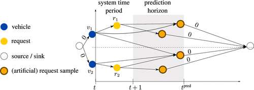
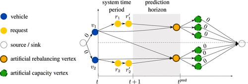
3.3. Rebalancing Actions
We recall that the so-far-introduced CO-enriched ML pipeline is rebalancing-agnostic. To circumvent this issue, we first extend a system state by enlarging its system time period with a prediction horizon , such that the system time period and the prediction horizon form an extended horizon. Second, we extend the vertex set V in the digraph D with artificial rebalancing vertices with . We locate these artificial rebalancing vertices in rebalancing cells.
3.3.1. Rebalancing Cells.
To derive rebalancing cells, we partition the fleet’s operating area into a rectangular grid, divided into equally sized squares, and refer to each square as a rebalancing cell (see Figure 3). Formally, we consider a square area covering the operating area. We can define this square area with the lower left corner point and the upper right corner point of this square: . Then, we partition this square horizontally and vertically into M equal-sized parts, yielding M2 rebalancing cells. We denote the set of rebalancing cells with C and denote one rebalancing cell with ; note . Thus, we can define a rebalancing cell ci with the lower left corner, and the upper right corner: . In this setting, we used squared rebalancing cells, but one can consider different shapes, for example, hexagons or other geographical boundaries, to partition the operating area.
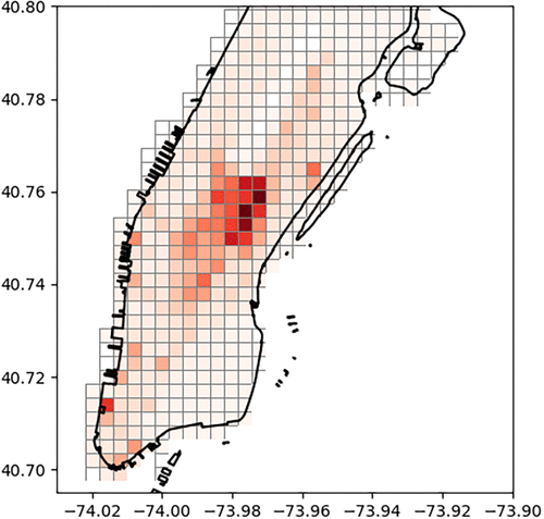
Note. Dark red color reflects a high probability for requests starting from this rebalancing cell.
Having defined rebalancing cells, we now introduce two modeling paradigms to allow for rebalancing actions: the SB paradigm and the CB paradigm. Both paradigms utilize the dispatching digraph and methodology as presented in Section 3.1, but differ in their modification techniques to adapt the digraph D to account for rebalancing. This enables us to solve the dispatching and rebalancing problem with the same approach as presented in Section 3.1. Whereas the SB modeling paradigm is a sampling-based approach that predicts artificial rebalancing vertices from a predefined distribution, the CB modeling paradigm is a model-free approach implicitly learning good rebalancing strategies to the center point of each rebalancing cell.
3.3.2. Sample-Based (SB) Paradigm.
The SB paradigm is a partially model-based approach that samples artificial rebalancing vertices from a request distribution calibrated on historical data and incorporates them into the digraph D as illustrated in Figure 4. Such an approach has proven to yield state-of-the-art results within related online algorithms (cf. Alonso-Mora et al. 2017). To do so, we derive the distribution of requests starting in an origin cell and ending in a destination cell for all cell pairs for a certain time interval I with a frequentist approach: we derive a table indexed by the time interval I, the origin rebalancing cell of a request , and the destination rebalancing cell of a request . Then, considering a time interval I within a week, for example, Monday between 8:00 a.m. and 8:15 a.m., we populate the table with historical requests. Specifically, we count the number of requests starting in an origin cell and ending in a destination cell for each origin-destination cell pair based on historical data for the respective interval I. Based on these observations, we calculate an interval-specific probability of the occurrence of a request with a specific origin-destination pair by dividing the number of observations for the respective origin-destination pair by the total number of requests that entered the system in the respective 15-minute interval I. Here, we define the probability of a request starting in origin cell co and ending in a destination cell cd at time interval I as
To use this distributional information in our SB pipeline, we further aggregate this information with respect to each origin cell by summing up the probabilities for each origin cell over all destination cells. Accordingly, we define the probability of a request starting in origin rebalancing cell co at time interval I as
Then, predicting the number of rebalancing vertices to place in rebalancing cell ci equals . We note that one can easily replace this sampling approach using the rebalancing cells with a more sophisticated predictor. This sophisticated predictor could, for example, directly predict the distribution of future requests. However, as the size of the rebalancing cells is usually rather small, the resulting accuracy increase using a more sophisticated predictor remains limited. We refer to the (SB) policy that results when incorporating the SB paradigm into the CO-enriched ML pipeline with δSB.
A key drawback of the SB paradigm and related sampling benchmarks (e.g., Alonso-Mora et al. 2017) is the dependency on distributional information for future ride requests. To avoid this, we propose a CB paradigm, which aims to extend the digraph with capacity vertices in each rebalancing cell, such that it is possible to learn distributional information when learning the digraph weights. In the following, we first provide the intuition behind the CB pipeline, and then detail each of its components.
3.3.3. Cell-Based (CB) Paradigm.
Instead of approximating rebalancing actions by sampling from historical data, we aim to learn the benefit of each rebalancing action with a model-free approach. To do so, we will include additional vertices and arcs in the digraph whose learnable weights are designed to align with the value of rebalancing one or multiple vehicles to each rebalancing cell. Clearly, the benefit of rebalancing vehicles to a rebalancing cell is not linear in the number of vehicles being sent to it. Hence, we rely on a discretization to model the benefit of each rebalancing vehicle, using multiple parallel arcs, each associated with a unique weight θi.
To embed such a multiarc representation, we still employ the k-dSPP on digraph D as introduced in Section 3.1, but solve an arc-disjoint instead of a node-disjoint k-dSPP. We add rebalancing vertices as schematically shown in Figure 5: we place one rebalancing vertex per rebalancing cell. The weights on the ingoing arcs to this rebalancing vertex represent the costs of a vehicle rebalancing to the respective cell. Then, we connect a rebalancing vertex with several artificial capacity vertices from and associate each arc pointing from a rebalancing vertex to an artificial capacity vertex i with a weight θi. We can interpret the weights to the artificial capacity vertices of the same rebalancing cell as the piecewise constant cost of each further vehicle rebalancing to the same rebalancing cell. By learning the weights on the ingoing arcs to the artificial capacity vertices, we implicitly learn the added cost of each further vehicle rebalancing into this rebalancing cell. Note that learning these weights also allows us to regulate the number of vehicles rebalancing to the same rebalancing cell.
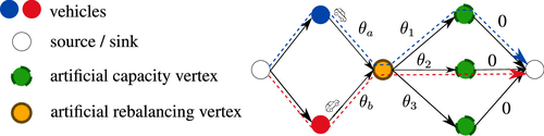
Notes. In an arc-disjoint k-dSPP, two vehicles rebalance to the same rebalancing cell. Both vehicles traverse the rebalancing vertex but a different capacity vertex, incurring respective costs of θ1 and θ2.
We use the technique described above to extend our digraph as shown in Figure 6: we add one rebalancing action as an artificial rebalancing vertex for each rebalancing cell and connect it to a set of artificial capacity vertices from . We refer to the digraph with artificial vertices as the extended digraph. Following this pipeline requires us to rethink our k-dSPP approach as we face the following conflict: in the created graph structure, multiple paths need to share a rebalancing vertex to learn the value of multiple rebalancing actions to the same location correctly. On the other hand, we still require paths to be vertex-disjoint with respect to request vertices to ensure dedicated request-to-vehicle assignments. To resolve this contradiction, we adapt the k-dSPP from finding vertex-disjoint paths to finding arc-disjoint paths, which allows paths to share a rebalancing vertex. To ensure disjoint request vertices between paths, we then split each request vertex into two vertices and introduce an arc with weight zero to connect both vertices. Then we can solve an arc-disjoint k-dSPP on the CO layer digraph. The resulting paths may share rebalancing vertices but are disjunct with respect to request and capacity vertices.
The advantage of the CB pipeline is that it embeds distributional information within the weights of the CO layer digraph and does not require any distributional information about future ride requests. We refer to the CB policy that results when incorporating the CB paradigm into the CO-enriched ML pipeline with δCB.
3.4. Decoder
The decoder receives k-disjoint paths, each representing a vehicle trip, and returns a dispatching and rebalancing action for each vehicle. When a vehicle path goes through r, we dispatch the vehicle to r if r is an actual request, that is, , and we rebalance the vehicle to the location of r if r is an artificial request, that is, .
3.5. ML Layer
We recall that the main rationale of the hybrid CO-enriched ML pipeline is to use an ML predictor to predict the weights of the CO layer digraph, such that solving the k-dSPP yields an anticipative dispatching and rebalancing solution. We predict the weight θa for each arc of the digraph using a generalized linear model, where is a features vector, which depends on arc a and system state x. Here, the system state x can also incorporate historical information. Additionally, we also tested a feedforward neural network (FNN), , as an ML predictor. Note that we detail the features used in the online supplement (Online Appendix D). Intuitively, in the SB pipeline, a weight on an artificial request’s ingoing arc represents the learned reward of rebalancing to the location of the artificial request. In the CB pipeline, the weight θa of each rebalancing vertex’s ingoing arc reflects the reward of a relocation to the respective rebalancing cell, and the weight of each capacity vertex’s ingoing arc reflects the reward of each additional vehicle rebalancing to this cell.
3.6. Structured Learning Methodology
The resulting policies δSB and δCB are clearly sensitive to the weights of the CO layer digraph . To effectively learn these weights θ, we leverage SL; that is, we aim at learning θ in a supervised fashion from past full-information solutions. To do so, we must derive a direct relation between the weights θ and the resulting policy decisions encoded via solution paths y. Therefore, we introduce the following notation: we denote a CO-layer-digraph as xi and embed the set of all feasible solutions in so that is a vector with
Then, we can formulate the CO layer problem, namely, the k-dSPP, as a maximization problem
Here, our goal is to find a θ such that leads to an efficient policy for all xi at our disposal. To do so, we use a learning-by-imitation approach. Practically, we build a training set containing n instances xi of the CO layer problem (6) as well as their solution that we want to imitate. We then formulate the learning problem as
3.6.1. Building the Training Set.
We aim to imitate an optimal full-information bound, which cannot be derived during online decision making because it requires information about future requests. Accordingly, we build a training set from historical data, which allows us to generate a training set based on full-information solutions. Our training set contains a training instance for each system time period of every problem instance at our disposal. We generate as follows: we solve the full-information problem of the respective historical problem instance for the complete problem time horizon. To do so, we modify the CO-enriched ML pipeline. In the digraph generator layer, we generate a digraph with all requests of this full-information problem. In the ML layer, we set the weights of a request’s ingoing arc according to the reward which the central controller receives for fulfilling the respective request. Subsequently, we solve the CO layer problem (6), which retrieves the full-information solution.
From the full-information problem instance, we rebuild the digraph xi of Problem (6) for the system time period of interest and assign the corresponding full-information solution to it. For a detailed elaboration on how we rebuild the digraph xi from a full-information problem instance and how we map the respective full-information solution on the digraph xi, including its rebalancing vertices, we refer to the online supplement (Online Appendix A).
3.6.2. Fenchel-Young Loss.
Given a training point , we want to find a θ such that the solution of Problem (6), namely , equals the optimal solution . It is therefore natural to use as loss the nonoptimality of as a full-information solution
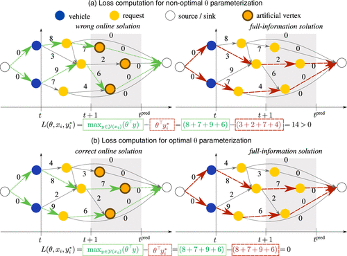
Notes. (a) Loss computation for some nonoptimal θ parameterization, based on the full-information solution (dashed red lines) and the solution computed based on θ (dotted green lines). As can be seen, we obtain a loss greater than zero. (b) Loss computation for optimal θ values, where the computed solution yields the full-information solution and the loss is zero.
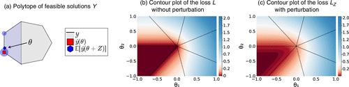
Unfortunately, the learning problem (7) combined with loss (8) contains a trivial solution with θ = 0. In this case, any feasible solution from is an optimal solution of the CO layer problem (6), which results in a random policy. We follow Berthet et al. (2020) and fix this issue by adding a Gaussian perturbation Z to θ, which has a regularizing effect,
Using the Fenchel duality interpretation of Berthet et al. (2020), this loss is equal to the left-hand side of the Fenchel-Young inequality
Figure 8 illustrates the effect of perturbing the loss function L. Intuitively, we consider a linear program with feasible solutions which represent a polytope (Figure 8(a)). The solution of the linear program is a vertex of this polytope (red square). Solving the linear program for various perturbations Z yields a set of solution vertices. The expectation over all solution vertices is in the relative interior of the feasible polytope , making it differentiable (blue hexagon). Now, focus on the loss function L of our learning problem: Figure 8(b) shows the loss value for different θ values. Note that the different cones represent the different vertices of the polytope presented in Figure 8(a). We see that the loss L is zero for many different values of θ, including . In Figure 8(c), we apply a perturbation Z and see that the loss LZ only becomes close to zero in the interior of the lower left cone, which allows deriving meaningful gradients when solving the respective learning problem.
3.6.3. Solving the Learning Problem.
An analysis based on Fenchel-Young convex duality enables us to show that this loss is smooth and convex (cf. Berthet et al. 2020) with the following gradient
For further discussion of smoothness and convexity properties and the gradient derivation, we refer to the online supplement (Online Appendix B).
Considering this gradient, we can minimize the learning problem (7), with loss (9) with respect to θ. As θ is a prediction of the ML predictor , we need to backpropagate the gradient through to learn w. To do so, the predictor must be differentiable. A straightforward differentiable predictor is a linear model
4. Experimental Design
This section details our experimental design by first introducing our real-world case study in Section 4.1 and afterward detailing our benchmark policies in Section 4.2.
4.1. Case Study
Our case study focuses on an online AMoD control problem for the New York City Taxi data set (New York City Taxi & Limousine Commission 2015) from the year 2015. We chose the year 2015 as it is the most recent year with exact recordings of starting and destination locations from ride requests, and restrict the simulation area to Manhattan. We model vehicle movements with exact longitude and latitude values. To avoid a computational overload for on-the-fly computation of driving times, we use a look-up table to retrieve the distance and the time needed to drive from a starting location to a destination location. We base this look-up table on data from Uber Movement for the year 2020 (data retrieved from Uber Movement, © 2022 Uber Technologies, Inc., https://movement.uber.com), which accounts for traffic conditions accordingly. Each location in this look-up table is specified by a rather small square cell of size 200 meters × 200 meters. If the starting and destination locations are in the same cell, we assume a line distance and an average driving speed of 20 kilometers per hour. The rebalancing cells are specified by larger square cells of size 333 meters × 333 meters to represent rebalancing areas.
We only consider weekdays as we assume different travel behavior on weekends, and focus on an AMoD system operating for one hour from 9:00 a.m. till 10:00 a.m. We assume a system time period of one minute such that the central controller can apply dispatching and rebalancing actions every minute. We split data into disjoint sets of training data, validation data, and testing data. The training data and the validation data comprise 5 working days × 1 hour of request data, and the testing data comprise 20 working days × 1 hour of request data. We stop the training after 70 training iterations or a maximum of 70 hours of training time. When discussing results, we report the averaged results over the testing data.
To further speed up the computation times of our k-dSPP algorithm, we apply sparsification techniques to sparsify the CO layer digraph. For a detailed description of this sparsification, we refer to the online supplement (Online Appendix E). For our specific case study, we finally only include an arc in the CO layer digraph if the distance to the next request is below 1.5 kilometers, and if the next request is reachable within 720.0 seconds. These thresholds permit us to significantly sparsen our digraph but have hardly any effect on the solution quality. Note that these thresholds are problem and instance specific and should be recalibrated for other use cases.
We generate different scenarios with varying fleet sizes ranging from 500 to 5,000 vehicles, and scenarios with different ride request densities, ranging from 10% to 100% of the original ride request volume. In each scenario, we optimize over profit and the number of satisfied customers. When we optimize over profit, we take the revenue for fulfilling the request extracted from New York City Taxi & Limousine Commission (2015) minus operational costs of 0.45$ per driven kilometer (Bösch et al. 2018). When we optimize over the number of satisfied customers, we take a revenue of one for fulfilling a ride request minus marginal costs of 0.00001 per driven kilometer, to retrieve a lexicographic objective that maximizes the number of satisfied ride requests but prefers sustainable solutions with fewer kilometers driven over less sustainable solutions. If not specified differently, we assume a base scenario that considers 30% of the original ride request volume and a vehicle fleet size of 2,000 vehicles. Here, we chose a request share of 30% to reflect a typical market share of a ride-hailing fleet (cf. Statista 2021). We then set the vehicle fleet size such that it enables a 100% request fulfillment under an optimal full-information approach. Note that we retrain the learning-based policies for each scenario.
4.1.1. Discussion.
A comment on the setup of this case study is in order. We experience that our CO-enriched ML pipeline leads to very general policies, shown by superior average performance over weekdays, although the request distribution might change from Monday to Friday. In this context, one may argue that demand patterns can change more drastically between different seasons, for example, from winter to summer, or weekday to weekend. For such cases, our analyses are still valid as one can easily either train separate models for drastically different scenarios or add context to the predictor to further enhance its generalizability.
4.2. Benchmark Policies
In our computational studies, we apply the following benchmark policies.
Greedy Policy: The greedy benchmark policy is an online policy that greedily reoptimizes dispatching decisions in a rolling horizon fashion. The greedy policy does not include any rebalancing vertices into the digraph and, instead of learning the weights of arcs in the digraph, sets the weight of a request’s ingoing arc according to its reward. Solving a k-dSPP on this digraph leads to greedy dispatching actions which only incorporate requests that are within the actual system time period.
Sampling Policy: The sampling benchmark policy is an online policy that reoptimizes dispatching and rebalancing decisions in a rolling horizon fashion and samples future requests for the prediction horizon from a request distribution calibrated on historical data. We derive this request distribution via the frequentist approach specified in Section 3.3. We can interpret the sampling policy also as a variant of a CO-enriched ML pipeline with a digraph generator that incorporates sampled ride requests as artificial rebalancing vertices in the digraph. Instead of learning the weights of arcs in the digraph, it sets the weight of a request’s ingoing arc according to its reward. To prefer real requests from the system time period over sampled requests from the prediction horizon, we multiply the reward of sampled ride requests with a discount factor of 0.2 as we received the best results for this factor. We consider a prediction horizon of four minutes as it leads to the best results (see Appendix F in the online supplemental material).
Full-Information Bound (FI): We compute a full-information bound with complete information about all ride requests. Solving the full-information problem optimally constitutes an upper bound for the online problem. To compute the full-information solution, we assume a system time period equal to the problem time horizon , such that all ride requests are available at the system at time t = 1. Accordingly, the digraph at t = 1 comprises all requests of the complete problem time horizon. Therefore, we do not have to predict the arc weights in the digraph but can set the arc weights of an arc equal to the reward for the ingoing request vertex.
SB Policy: The SB policy is an online policy that follows the variant of the CO-enriched ML pipeline presented in Section 3.3. The policy reoptimizes dispatching and rebalancing actions in a rolling horizon fashion. For the SB policy, we consider a prediction horizon of four minutes, as we received the best results for this planning horizon (see Appendix G in the online supplemental material).
CB Policy: The CB policy is an online policy that follows the variant of the CO-enriched ML pipeline presented in Section 3.3. The policy reoptimizes dispatching and rebalancing actions in a rolling horizon fashion. We set the number of capacity vertices for every rebalancing cell to one, as we achieved the best results with this setting. For the CB policy, we consider a prediction horizon of four minutes, as we received the best results for this planning horizon (see Appendix G in the online supplemental material).
5. Results
In the following, we first present the results of the real-world case study for different vehicle fleet sizes and request densities in Section 5.1. We then provide an in-depth structural analysis for the SB and CB policies and compare them with the other benchmark policies with respect to external effects and computational time in Section 5.2.
5.1. Performance Analysis
To analyze the performance of our learning-based policies, we benchmark their performance for various scenarios with varying fleet sizes and request densities as well as for varying objectives, first focusing on profit maximization.
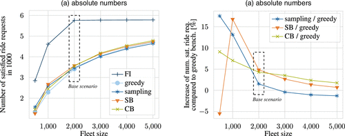
5.1.1. Varying Fleet Size.
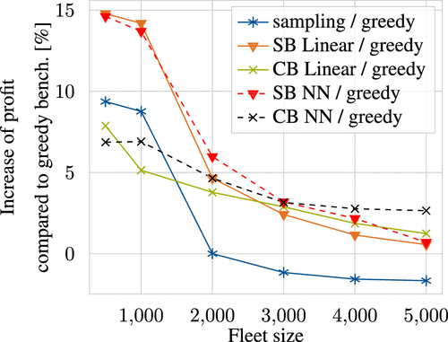
Figure 9 shows the performance of the SB policy and the CB policy compared with the greedy and sampling policies, and with the full-information bound for different fleet sizes when maximizing the profit. Here, the data point with a fleet size of 2,000 vehicles constitutes our base scenario. As can be seen, there is a significant gap between the full-information bound, which remains an upper bound, and all other policies; see Figure 9(a). This gap reduces for increasing or decreasing fleet sizes as in the former case, the assignment of requests to vehicles gets less error sensitive, whereas in the latter case, the objective value of the full-information solution decreases overproportionally because of the reduced solution space. The significant gap between the full-information bound and the online benchmarks derives from the rolling horizon approach: although the full-information policy allows us to find dispatching solutions independent of the time discretization, some dispatching solutions might turn infeasible with time discretization as idling vehicles cannot rebalance to unknown future ride requests.
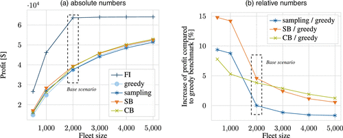
To ease the comparison between all online policies, Figure 9(b) compares both the SB and the CB policies as well as the sampling policy against the greedy policy. In the base scenario, both the SB and CB policies outperform the greedy and the sampling policies: whereas the SB policy improves upon the greedy policy by 4.6%, the CB policy improves upon the greedy policy by 3.8%, and the sampling policy matches the performance of the greedy policy. For increasing fleet sizes, the performance difference between the SB and CB policies decreases. Remarkably, the sampling policy performs even worse than the greedy policy in these cases. This deteriorating performance of the sampling policy results from the following dynamics: for large fleet sizes, the sampling policy leads to unnecessary rebalancing actions that cause additional cost. With increasing fleet size, the vehicle density in the operating area and, accordingly, the probability that a vehicle is close to a future request increase without taking further rebalancing actions. As a consequence the greedy policy yields better assignments for larger fleet sizes but does not incur additional rebalancing costs, which leads to an overall profit that exceeds the one reached when applying the sampling policy. For decreasing fleet sizes, all policies show an increased performance gain compared with the greedy policy as the anticipation and prioritization of profitable requests are even more crucial in this setting. Here, the SB policy still outperforms all other policies but the sampling policy shows a larger improvement compared with the CB policy. These results indicate that the CO-enriched ML pipeline outperforms the sampling benchmark, which is similar to the model-predictive control approach of Alonso-Mora et al. (2017). Note that a recent DRL algorithm only outperforms greedy policies in similar settings by around 2%–5% (cf. Enders et al. 2023).
Both the SB and CB policies robustly improve over the greedy policy, whereas the sampling policy shows a fragile performance, often performing worse than the greedy policy. The SB policy outperforms all other policies with improvements over the greedy policy of up to 14.8%. The CB policy outperforms the sampling policy in most scenarios, although the CB policy does not require distributional information on future ride requests.
5.1.2. Varying Request Density.
Figure 10 extends our performance analysis by showing the performance of all different policies for different request densities when fixing the number of vehicles to 2,000. For scenarios with a higher request density than in our base scenario, the SB policy outperforms all other online policies with average improvements of 13.1% compared with a greedy policy. The sampling policy shows average improvements of 10.3% for increasing request densities. For decreasing request densities, the sampling policy performs even worse than the greedy policy.
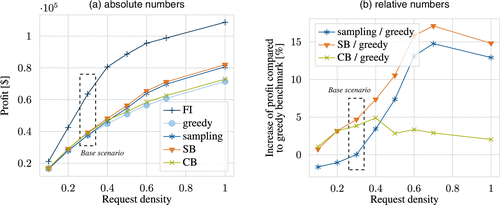
Unsurprisingly, the sampling policy does not perform as well on low request densities as it does on high request densities. Indeed, it relies on a single sampled scenario to take decisions. When there are very few requests, a single scenario can be seen as mostly noise and does not provide accurate information on the distribution of requests. Addressing this issue with a sampling-based approach would require sampling several scenarios, which would lead to a two-stage stochastic formulation. Such a formulation would make the policy much more computationally intensive, and difficult to apply in practice. On the contrary, our CB and SB policies robustly perform better than the greedy policy also for low request densities. This holds even for the SB policy, although it inherits the same weakness as the sampling policy as it samples rebalancing locations. This shows the robustness of our learning-based policies compared with the sampling policy, and further indicates their superiority in terms of solution quality.
The CB and SB policies yield a stable performance and improve upon the greedy policy across all request densities. Contrarily, the sampling policy performs well on high request densities but badly on low request densities.
5.1.3. Maximizing Number of Satisfied Customers.
Figure 11 extends our analysis to a different objective and shows the performance of all policies for a varying fleet size when maximizing the number of satisfied ride requests. As can be seen, our SB policy outperforms all other policies, improving by up to 16.8% compared with a greedy policy for fleet sizes between 1,000 and 5,000 vehicles. Again, we observe that the difference between a greedy policy and our learning-based policies decreases for increasing fleet sizes, whereas the sampling policy performs even worse than a greedy policy in such cases. However, we also observe one outlier: although our SB policy performs worse than the greedy policy in the artificial case of 500 vehicles, the sampling policy outperforms the greedy policy in this case. This is because in this case, the request-to-vehicle ratio is very large such that the pure information about possibly available requests, which we obtain by sampling, suffices to achieve a good algorithmic performance. This is particularly possible because any request—independent of its duration or cost—adds the same contribution to the objective when solely maximizing the number of satisfied requests. Note that we observe a completely opposite behavior as soon as we change the objective toward a request-sensitive target when optimizing the total profit (cf. Figure 9(b)): in this case, the SB policy yields an improvement of 14.8% compared with a greedy policy as the learning allows us to estimate the value of potential future requests.
Our SB policy outperforms all other online policies across different objectives and various scenarios that reflect real-world applications. Our CB policy yields lower improvements than our SB policy, but shows a more robust performance for artificial corner cases.
5.1.4. Conclusion.
Our results show that our learning-based policies outperform a greedy and a sampling policy across varying objectives and scenarios with different fleet sizes and request densities. In particular, our SB policy yields improvements up to 17.1% compared with a greedy policy for scenarios that reflect real-world applications. In these cases, our CB policy improves upon a greedy policy up to 9.1%, whereas a sampling policy shows an unstable performance that sometimes yields improvements, but oftentimes performs even worse than a greedy policy. In artificial corner cases, our SB policy may also perform worse than a greedy policy as it by design inherits some of the structural difficulties of any sampling-based approach. Here, our CB policy still shows a robust performance that improves upon a greedy policy.
To conclude from a technical perspective, one can generally interpret the SB approach as a partially model-based approach because it assumes knowledge of a future request distribution. This distribution is used to sample future requests, enabling rebalancing. In contrast, the CB approach is model-free, as it does not rely on a predefined request distribution for rebalancing. Instead, the CB approach implicitly learns this distribution during training. Intuitively, whereas the SB policy leverages prior information about the request distribution, the CB policy outsources this knowledge to the learning process.
The primary advantage of the SB approach is its superior performance across most scenarios, provided the request distribution is known. This explains the superior performance of the SB approach in our experiments as it has access to the empirical distribution by accessing historical data. Conversely, the CB approach excels in scenarios where no prior knowledge of the request distribution is available. Accordingly, one may observe different results for application cases where the available empirical distribution is noisy or unknown.
5.2. Extended Analysis
In the following, we deepen our analyses of the differences between the proposed benchmark policies. To this end, we analyze structural differences between the different policies and discuss their impact on external effects, as well as their efficiency with respect to computational times.
5.2.1. Structural Policy Properties.
Figure 12 shows the evolution of the vehicle distribution for a representative instance over different points in time for the different benchmark policies. We interpret this evolution of vehicle distributions as an indicator of how the respective benchmark policies differ in their dispatching and rebalancing behavior, and refer to our GitHub repository (Jungel et al. 2025) for an interactive visualization of idling, dispatching, and rebalancing characteristics of all policies. Compared with the full-information bound, the sampling policy leads to a compressed vehicle distribution in the city center, which occurs because of a biased rebalancing behavior that overvalues high-request-density areas over low-request-density areas. This leads to a significant number of vehicles idling in high-request-density areas, which leads to missed requests in mid- to low-density areas and worsens the policy’s performance. The SB policy also shows a vehicle distribution that revolves around the city center and its high-request-density areas, which results from the fact that both policies leverage the identical historical request distribution for sampling future ride requests. However, the SL element allows anticipating better the value of relocations, which leads to vehicle distributions that still revolve around high-request-density areas but distribute a significantly larger share of vehicles to mid- and low-density areas, which yields the performance improvement of our SB policy. The CB policy leads to a slightly more uniform vehicle distribution over the operating area as, by design, it restricts the maximum number of vehicles rebalancing to a rebalancing cell via the number of capacity vertices in each rebalancing cell. With these rebalancing actions, the CB policy yields a performance that is always better than greedy but remains below the performance of the SB policy.
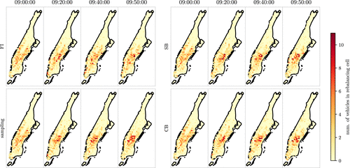
Whereas sample-based policies tend to rebalance too many vehicles to high-request-density areas, CB policies lead to a slightly more distributed rebalancing.
5.2.2. Externalities.
Figure 13 shows the externalities of our online policies compared with a greedy policy for different fleet sizes when optimizing the total profit. Here, we particularly focus on the number of served requests, the average number of kilometers driven per request, and the average number of kilometers driven per vehicle. As can be seen, the increase in the number of served requests is proportional to the profit increase for each policy. Accordingly, the SB policy yields the highest improvement for the number of served customers, and thus contributes to increase customer satisfaction. Remarkably, the SB policy yields a lower increase of average kilometers per request and per vehicle than the sampling policy, while at the same time yielding a higher number of passengers served and a higher profit. This highlights the efficacy of the SB policy, even for key performance indicators that are anticorrelated. We note that the SB policy still yields higher average kilometers driven per request and vehicle than the CB and greedy policies for small fleet sizes. This is because these policies show a significantly lower performance on the anticorrelated key performance indicators, such as the number of satisfied requests and the total profit. For scenarios with large fleet sizes, when the SB and CB policies lead to a similar performance with regard to total profit, also the KPIs for average kilometers driven per request and vehicle are similar.
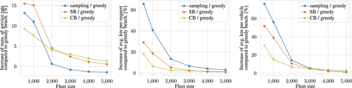
The SB policy yields a good trade-off between anticorrelated key performance indicators and outperforms the sampling policy on both the number of satisfied customers and the total profit as well as on the distance driven per request and vehicle.
5.2.3. Computational Time.
Table 1 presents the average computational time to compute dispatching and rebalancing actions for all benchmark policies. We consider a system time period of one minute for all online policies and do not incorporate the time to construct the digraph. As can be seen, all policies benefit from the polynomial algorithm introduced in Section 3.1. Although the greedy policy shows lower computational times compared with the sampling and learning-based policies, all online policies show computational times below a few seconds, which allow for application in practice when operating an AMoD system with a one-minute system time period. Note that the time to solve the full-information problem equals the time to generate offline data, which are then used to generate training data. The time for retrieving the training data from the offline data is negligible.
|

Table 1. Average Computational Time (Seconds) to Calculate Dispatching and Rebalancing Actions
| Fleet size | ||||||
|---|---|---|---|---|---|---|
| 500 | 1,000 | 2,000 | 3,000 | 4,000 | 5,000 | |
| FI | 2.314 | 4.396 | 10.155 | 14.949 | 27.59 | 28.792 |
| Greedy | 0.012 | 0.05 | 0.208 | 0.485 | 0.863 | 1.384 |
| Sampling | 0.041 | 0.169 | 0.588 | 1.201 | 2.003 | 3.01 |
| SB | 0.069 | 0.179 | 0.576 | 1.186 | 2.025 | 3.038 |
| CB | 0.093 | 0.312 | 0.905 | 1.798 | 2.966 | 4.167 |
5.2.4. Deep Learning ML Layer.
In the previous results, we used a linear predictor in the ML layer to predict the digraph weights θ, according to Equation (12). Instead of using a linear predictor, we can also use a differentiable deep learning predictor of the general form . For learning a deep learning predictor, some adaptions are in order in comparison with learning a linear predictor. First, instead of using the BFGS method, we use a stochastic gradient descent (SGD) method to optimize the learning problem (7). Second, the SGD method updates the weights w for each training instance instead of updating the weights with a mean gradient over all training instances. Third, for deriving a subgradient (11), we add a perturbation Z to θ instead of perturbing the weights w.
Figure 14 shows the performances of the CO-enriched ML pipeline for different vehicle fleet sizes when using an FNN predictor and a linear predictor. We tuned the hyperparameters of the FNN, for example, the learning rate, and the network architecture individually in each scenario. Surprisingly, the CO-enriched ML pipeline including the FNN does not outperform the pipeline including the linear predictor in all scenarios: in scenarios with a small vehicle fleet size, the linear predictor leads to better performance. This is due to an overfitting issue of the FNN on the training data, which we detail in the supplemental material (Online Appendix H). In all other scenarios, the FNN leads to a slightly better performance. Note that we visualize the learning curves of the linear predictor and the deep learning predictor for the SB and CB policies in the supplemental material (Online Appendix I).
The FNN predictor in the ML layer improves the performance of the CO-enriched ML pipeline in most scenarios. However, the CO-enriched ML pipeline including the FNN does not generalize well for all scenarios.
6. Conclusion
In this paper, we introduced a new family of online control policies for dispatching and rebalancing decisions in AMoD fleets. To derive such policies, we presented a novel CO-enriched ML pipeline that learns prescriptive dispatching and rebalancing decisions from full-information solutions. To establish this pipeline for our particular application case, we showed how to solve the underlying CO problem in polynomial time, how to leverage SL to learn a parameterization for the CO problem such that it allows for prescriptive dispatching and rebalancing actions, and how to derive corresponding learning-based control policies.
We presented a profound numerical study based on a real-world case study for Manhattan to show the efficacy of our learning-based policies and benchmark them against a greedy policy and a sampling-based receding horizon approach (cf. Alonso-Mora et al. 2017). Our results show that the sampling policy has an unstable performance and oftentimes performs even worse than the greedy policy. The performance of the sampling policy is in line with the performance of other benchmarks, for example, DRL algorithms, that reach an improvement of up to 5% over myopic policies in similar settings. Our learning-based policies show a significant improvement over such approaches, yielding improvements over a greedy policy of up to 17.1%. Moreover, our learning-based policies are robust and always outperform the greedy policy. Finally, our learning-based policies yield a good trade-off between anticorrelated key performance indicators; for example, when maximizing the total profit or the number of served customers, we still obtain a lower distance driven per vehicle compared with policies that show worse performance on the aforementioned quantities.
The presented CO-enriched ML pipeline paves a promising avenue for future research in the realm of online control policies. In future work, we aim to extend the CO-enriched ML pipeline to account for stochastic travel times using point-based estimators and continuous waiting times.
References
- (2017) Predictive routing for autonomous mobility-on-demand systems with ride-sharing. 2017 IEEE/RSJ Internat. Conf. Intelligent Robots Systems (IROS) (IEEE, New York), 3583–3590.Google Scholar
- (2021) Machine learning for combinatorial optimization: A methodological tour d’horizon. Eur. J. Oper. Res. 290(2):405–421.Crossref, Google Scholar
- (2020) Learning with differentiable perturbed optimizers. Larochelle H, Ranzato M, Hadsell R, Balcan M, Lin H, eds. Advances in Neural Information Processing Systems, vol. 33 (Curran Associates, Inc., Red Hook, NY), 9508–9519.Google Scholar
- (2019) Online vehicle routing: The edge of optimization in large-scale applications. Oper. Res. 67(1):143–162.Link, Google Scholar
- (2018) Cost-based analysis of autonomous mobility services. Transport Policy 64:76–91.Crossref, Google Scholar
- (2022) Learning with combinatorial optimization layers: A probabilistic approach. Preprint, submitted July 27, https://arxiv.org/abs/2207.13513.Google Scholar
- (2017) Task-based end-to-end model learning in stochastic optimization. Guyon I, Von Luxburg U, Bengio S, Wallach H, Fergus R, Vishwanathan S, Garnett R, eds. Advances in Neural Information Processing Systems, vol. 30 (Curran Associates, Inc., Red Hook, NY), 5484–5494.Google Scholar
- (2022) Smart “predict, then optimize.” Management Sci. 68(1):9–26.Link, Google Scholar
- (2023) Hybrid multi-agent deep reinforcement learning for autonomous mobility on demand systems. Matni N, Morari M, Pappas GJ, eds. Proc. 5th Annual Learn. Dynam. Control Conf., Proceedings of Machine Learning Research, vol. 211 (PMLR, New York), 1284–1296.Google Scholar
- (2021) Graph neural network reinforcement learning for autonomous mobility-on-demand systems. 2021 60th IEEE Conf. Decision Control (CDC) (IEEE, New York), 2996–3003.Google Scholar
- (2018) Data-driven model predictive control of autonomous mobility-on-demand systems. 2018 IEEE Internat. Conf. Robotics Automation (ICRA) (IEEE, New York), 6019–6025.Google Scholar
- (2021) Real-world ride-hailing vehicle repositioning using deep reinforcement learning. Transportation Res. Part C Emerging Tech. 130:103289.Crossref, Google Scholar
- (2025) Learning-based online optimization for autonomous mobility-on-demand fleet control. https://doi.org/10.1287/ijoc.2024.0637.cd, https://github.com/INFORMSJoC/2024.0637.Google Scholar
- (2021) End-to-end constrained optimization learning: A survey. Zhou ZH, ed., Proc. 30th Internat. Joint Conf. Artificial Intelligence IJCAI-21 (International Joint Conferences on Artificial Intelligence Organization), 4475–4482.Google Scholar
- (2010) Evaluation of the public health impacts of traffic congestion: A health risk assessment. Environ. Health 9(1):65.Crossref, Google Scholar
- (2019) Efficient ridesharing order dispatching with mean field multi-agent reinforcement learning. World Wide Web Conf. (Association for Computing Machinery, New York), 983–994.Google Scholar
- (2022) An integrated reinforcement learning and centralized programming approach for online taxi dispatching. IEEE Trans. Neural Networks Learn. Systems 33(9):4742–4756.Crossref, Google Scholar
- (2022) Proactive rebalancing and speed-up techniques for on-demand high capacity ridesourcing services. IEEE Trans. Intelligent Transportation Systems 23(2):819–826.Crossref, Google Scholar
New York City Taxi & Limousine Commission (2015) TLC trip record data. https://www1.nyc.gov/site/tlc/about/tlc-trip-record-data.page.Google Scholar- (2011) Structured learning and prediction in computer vision. Foundations Trends Comput. Graphics Vision 6(3–4):185–365.Crossref, Google Scholar
- (2021) Learning to approximate industrial problems by operations research classic problems. Oper. Res. 70(1):606–623.Link, Google Scholar
- (2023) Structured learning based heuristics to solve the single machine scheduling problem with release times and sum of completion times. Eur. J. Oper. Res. 305(3):1032–1041.Crossref, Google Scholar
- (2015)
Autonomous mobility-on-demand systems for future urban mobility . Maurer M, Gerdes J, Lenz B, Winner H, eds. Autonomes Fahren (Springer, Berlin), 399–416.Crossref, Google Scholar - (2012) Robotic load balancing for mobility-on-demand systems. Internat. J. Robotics Res. 31(7):839–854.Crossref, Google Scholar
- (2022) Reinforcement learning in the wild: Scalable RL dispatching algorithm deployed in ridehailing marketplace. KDD ‘22 Proc. 28th ACM SIGKDD Conf. Knowledge Discovery Data Mining (Association for Computing Machinery, New York), 3838–3848.Google Scholar
- (2021) A polynomial-time algorithm for user-based relocation in free-floating car sharing systems. Transportation Res. Part B Methodological 143:65–85.Crossref, Google Scholar
- (2019) 2019 urban mobility report. Technical report, Texas A&M Transportation Institute, College Station.Google Scholar
- (2022) A modular and transferable reinforcement learning framework for the fleet rebalancing problem. IEEE Trans. Intelligent Transportation Systems 23(8):11903–11916.Crossref, Google Scholar
Statista (2021) Market share of the leading ride-hailing companies in the United States from September 2017 to July 2021. https://www.statista.com/statistics/910704/market-share-of-rideshare-companies-united-states/.Google Scholar- (2019) A deep value-network based approach for multi-driver order dispatching. KDD ‘19 Proc. 25th ACM SIGKDD Internat. Conf. Knowledge Discovery Data Mining (Association for Computing Machinery, New York), 1780–1790.Google Scholar
- (2018) Stochastic model predictive control for autonomous mobility on demand. 2018 21st Internat. Conf. Intelligent Transportation Systems (ITSC) (IEEE, New York), 3941–3948.Google Scholar
- (2020) A concise guide to existing and emerging vehicle routing problem variants. Eur. J. Oper. Res. 286(2):401–416.Crossref, Google Scholar
- (2020) Waymo opens driverless robo-taxi service to the public in Phoenix. Reuters (October 8), https://www.reuters.com/article/us-waymo-autonomous-phoenix-idUKKBN26T2Y3.Google Scholar
- (2018) Large-scale order dispatch in on-demand ride-hailing platforms: A learning and planning approach. KDD ‘18 Proc. 24th ACM SIGKDD Internat. Conf. Knowledge Discovery Data Mining (Association for Computing Machinery, New York), 905–913.Google Scholar
- (2022) Analysis and control of autonomous mobility-on-demand systems. Annual Rev. Control Robotics Autonomous Systems 5(1):633–658.Crossref, Google Scholar
- (2016) Control of robotic mobility-on-demand systems: A queueing-theoretical perspective. Internat. J. Robotics Res. 35(1–3):186–203.Crossref, Google Scholar
- (2019) Multi-agent reinforcement learning for order-dispatching via order-vehicle distribution matching. CIKM ‘19 Proc. 28th ACM Internat. Conf. Inform. Knowledge Management (Association for Computing Machinery, New York), 2645–2653.Google Scholar