


Demand Estimation Using Managerial Responses to Automated Price Recommendations
Abstract
We provide a new framework to identify demand elasticities in markets where managers rely on algorithmic recommendations for price setting and apply it to a data set containing bookings for a sample of midsized hotels in Europe. Using nonbinding algorithmic price recommendations and observed delay in price adjustments by decision makers, we demonstrate that a control-function approach, combined with state-of-the-art model-selection techniques, can be used to isolate exogenous price variation and identify demand elasticities across hotel room types and over time. We confirm these elasticity estimates with a difference-in-differences approach that leverages the same delays in price adjustments by decision makers. However, the difference-in-differences estimates are more noisy and only yield consistent estimates if data are pooled across hotels. We then apply our control-function approach to two classic questions in the dynamic pricing literature: the evolution of price elasticity of demand over and the effects of a transitory price change on future demand due to the presence of strategic buyers. Finally, we discuss how our empirical framework can be applied directly to other decision-making situations in which recommendation systems are used.
This paper was accepted by Omar Besbes, revenue management and market analytics.
Funding: D. Garcia acknowledges financial support from the Austrian Science Fund [Single Project “Understanding Consumer Search” FWF-P 30922].
Supplemental Material: The online appendix and data are available at https://doi.org/10.1287/mnsc.2021.4261.
1. Introduction
Revenue management provides a toolkit for sellers to optimally price goods with uncertain demand and fixed capacity. By combining rigorous statistical methods with business applications, the discipline has become a resounding success and is now a standard tool in multiple industries. In the classical framework, firms adjust prices over time in response to the arrival of new consumers with uncertain demand, taking into account the opportunity cost of selling an additional unit (Talluri and van Ryzin 2004, Phillips 2005). In addition to accurate demand forecasting, optimal pricing also requires precise knowledge of the marginal effect a (transitory) price change has on the final quantity sold of a given item. In this paper, we provide a novel approach to causally estimate price elasticities of demand that can be used in static as well as dynamic settings. The estimation approach is particularly well suited for environments that require controlling for a large number of potentially confounding variables. We demonstrate its strength in an application to dynamic hotel room pricing, using a data set that contains all bookings, prices, and algorithmic price recommendations for nine European hotels for a period of 14 months. Our application is directly relevant for revenue management in the hospitality industry, one of the largest sectors in the worldwide economy.1 The approach can also be applied to an array of decision problems that rely on recommendation systems outside our specific application.
Unlike standard ways of estimating demand, our method leverages demand shocks rather than cost shocks. This difference is important, especially in the service and financial sectors, in which demand shocks are frequent, whereas cost shocks are rare and often hard to identify. Consequently, estimating demand is notoriously difficult in these industries. The problem is exacerbated by managers increasing prices in periods of high demand, inducing a positive correlation between prices and sales (Bajari et al. 2015, Athey 2017). In the hotel industry, our main focus, this correlation has been widely documented using market-level and hotel-level data (e.g., Enz and Canina 2010 and Cho et al. 2018). Our approach offers an alternative to cost-shock-based methods in situations where those cost shocks are not available, and it produces plausible negative elasticities when traditional methods fail to do so. It can therefore be used in practice, allowing revenue managers to set prices more accurately, as well as by researchers who require accurate demand elasticities as parameters in their models of competition and industry-level welfare.
Our identification strategy rests on the ability to observe prices adjusting with delay to demand shocks. Intuitively, holding demand constant on its new, postshock level, the difference in sales before and after the price change informs us of the price elasticity of demand. Such variation is abundantly available in industries that rely on price-recommendation systems for pricing decisions (e.g., the accommodation, transportation, car rental, and other inventory-management industries). We show in our application to hotel room pricing that hoteliers follow the algorithmic recommendations very closely, but do so with a delay, thereby generating exactly the type of variation required by our estimation approach.
The above identification strategy suggests a simple difference-in-differences estimator that compares sales in a period after the recommended price change, but before the actual price change has been implemented, to sales in a period following the actual price change. As a first step, we implement this simple method and show, using both real-world and simulated data, that it produces accurate demand estimates when there are enough purchasing events within a short interval around the time of the actual price change. However, the frequency of purchasing events in our sample is relatively low, which leads to noisy estimates. We conclude that the difference-in-differences estimator is only appropriate for pricing homogeneous products that are purchased frequently and in relatively large quantities. In contrast, the estimates are too inaccurate for pricing hotel rooms, whose demand varies by room type, location, and across seasons.
We remedy the low efficiency of the difference-in-differences estimator by applying a high-dimensional control-function approach for causal inference developed recently in the machine-learning literature (Belloni et al. 2014). It allows us to use all of the relative variation on prices and price recommendations and all of the purchasing events while flexibly controlling for a large number of potential omitted variables. This approach provides accurate estimates, even at the level of a single room type for a single season. Furthermore, compared with structurally modeling demand and the response of hotel managers to recommendations, the method is less susceptible to functional misspecification because it allows for a high-dimensional set of competing functional forms. The results from the control-function approach agree with the difference-in-differences results on the pooled data, which makes us also confident in its ability to measure price elasticities accurately at the room-type level. We further demonstrate the robustness and accuracy of the results with simulations even for the case in which the model is misspecified.
Our approach is related to recent attempts to obtain causal inference on managerial decisions in various industries, such as ride-sharing (Cohen et al. 2016, Castillo 2019), staffing (Mani et al. 2015), and loan markets (Costello et al. 2020); each of these papers exploits a specific institutional or technological feature that generates exogenous variation in the implemented policy. In contrast, our estimation approach uses a “behavioral reaction” of managers that can be applied potentially in many other contexts in which decisions are based on algorithmic recommendations. For example, it could be used to estimate the expected marginal value of inventory in retail applications, where an inventory-management system recommends restocking times and quantities to a local store manager (Conlon and Mortimer 2013, Cachon et al. 2019)2; see Section 3.2 for more examples.
In our application, we extend our estimation framework and investigate two aspects of intertemporal demand important for optimal pricing in dynamic settings. First, we estimate how much the demand elasticity for hotel rooms varies over the booking horizon. Note that if the demand elasticity was constant over different booking horizons, then revenue-maximizing prices would tend to decrease as the day of arrival approaches, because the opportunity cost of an unsold room is decreasing over time. Instead, our results reveal that prices are roughly constant, suggesting increasing markups. In particular, the price sensitivity (semielasticity) of consumers is highest for very early bookers and lowest for those buying between 21 and 50 days before the date of stay. Overall, our findings are consistent with the idea that consumers who are more price-sensitive search early on. Our results also corroborate evidence from airline tickets (Williams 2022) and help in reconciling the profile of constant or increasing prices with decreasing opportunity costs.
Second, we measure to what extent hotel customers delay their purchase when facing a higher price. To answer this question, we follow ideas in Li et al. (2014), who estimate strategic consumer behavior in the market for airline tickets and include lagged prices to identify the effect of variation in past prices on current demand.3 We show that past prices have lasting effects on current demand, but these effects vary across hotels. For one of the hotels in our sample, high past prices are likely to discourage searchers, reducing current demand, whereas for another hotel, the pattern is reversed.
In summary, we provide in this paper a new reduced-form regression approach to identify demand elasticities in markets with dynamic demand and a limited access to observable supply shocks. In an application to hotel-room pricing, we then study the variation in demand elasticity as the day of arrival approaches and the impact of strategic consumers on optimal pricing. An advantage of our approach is that it provides, in contrast to other methods, reliable estimates for relatively small sample sizes and circumvents the need for experimental variation (e.g., Moon et al. 2018 and Nambiar et al. 2019) or structural modeling (e.g., Li et al. 2014 and Cho et al. 2018). A key innovation of our approach is that it leverages recommended rates produced by an advanced pricing algorithm and the associated behavioral responses of managers to this kind of information.
1.1. Contribution to the Literature
Our contribution to the literature is twofold. First, we provide a simple, yet powerful, approach to estimate demand leveraging on recommendation data that are very often available to decision makers. The approach combines machine-learning algorithms with modern causal-inference methods (Belloni et al. 2014, Chernozhukov et al. 2015, Belloni et al. 2016). The only paper we are aware of that uses similar ideas for identifying demand is the contemporaneous work by Castillo (2019). We both use a reduced-form approach, isolating short-run price changes, which are arguably uncorrelated with both demand and supply. Castillo (2019) exploits discontinuities in the specific price-setting algorithm of a ride-hailing company to identify customers’ willingness-to-pay. Instead, we use sluggish price adjustment by managers as the source of exogenous variation. The “behavioral response” can be applied in a broad range of settings, from estimating the marginal impact of an additional worker in a retail store to the foregone profits due to stock-outs, as discussed in Section 3.2.
Our second main contribution concerns an application to hotel-room pricing (see Section 5). Extending our estimation approach, we address two questions relevant for optimal dynamic pricing: How does the price sensitivity of demand change over time, and what is the effect of a price change on behavior of forward-looking consumers? To the best of our knowledge, only a handful of papers attempt to estimate demand in dynamic markets. These include Li et al. (2014), Lazarev (2013), and Williams (2022), who study the market for airline tickets; Joo et al. (2020) in the holiday cruise industry; and Li et al. (2018) and Cho et al. (2018), who, like us, focus on dynamic pricing in the hotel industry. Most of them resort to structural modeling to estimate dynamic demand.4
In the first application, we recover time-varying demand elasticities for the biggest hotels in our sample. In a related work, Williams (2022) develops a structural model and identifies the consumer demand elasticity over time, as well as the welfare implications of dynamic pricing, by combining posted prices of airline tickets and flight-availability data from aircraft seat maps. Lazarev (2013) uses a high-frequency data set on airfares to study the welfare effects of dynamic pricing in a structural model, which also allows for individuals to learn about their travel needs by delaying purchases. They both find that earlier consumers are more price-sensitive. An exception is the recent work by Joo et al. (2020), who estimate demand for holiday cruises, using a cost shock for identification, and find that demand becomes more elastic as the departure date approaches.
The second application concerns the role of forward-looking consumers. Whereas the classical dynamic pricing literature assumed that consumers act myopically, there has been a growing interest in the theoretical literature on strategic, or forward-looking, behavior of consumers in dynamic settings. Our empirical results are hence not only of interest for practitioners, but can also inform theoretical work on optimal dynamic pricing.5 To our knowledge, there are very few papers that try to identify the presence of strategic consumers; most of them rely on structural identification using data from the airline industry. In terms of magnitudes, our results are broadly consistent with those of Li et al. (2014) and suggest that, for the biggest hotel in our sample, approximately one-third of consumers are willing to delay their purchasing decisions in the hope of obtaining a better price in the future.
2. Data and Institutional Background
Our data set contains more than 5 million observations of hotel-room pricing information and the corresponding universe of about 60,000 bookings, all aggregated at the daily level. This high-resolution proprietary data set was made available by our corporate sponsor, whose identity is withheld by request. The corporate sponsor is based in Europe and provides a number of revenue-management services, including price recommendations, to a large number of independent hotels. The rate and booking data come from nine different hotels, eight located at resort destinations and one (hotel 6) located in an urban area. Our data contain bookings and prices for each hotel over a period of about 14 months. For each potential arrival date, we observe the flow of bookings, actual rates charged by the hotel, and rates recommended for every room by the revenue-management company. The actual rate can be thought of as an index price set by the hotel. It is modified by prespecified and channel-specific discounts or fees and is then pushed to each channel in which the product is offered. We also include the actual rate in our analysis because both the revenue-management system (RMS) and the hotelier use this variable as the main instrument for price optimization.6 In addition, we observe for each booking the unique customer identifier, date of booking, date of arrival, length of stay, and the total price paid by a customer, as can be seen from Table 1.
|

Table 1. Summary Statistics of Rates and Bookings by Room Category
| Variable | Single | Standard | Superior | Suite |
|---|---|---|---|---|
| Actual rate | 81.56 | 160.53 | 173.94 | 210.61 |
| Actual rate (conditional on booking) | 81.34 | 159.35 | 168.88 | 198.75 |
| Total price per night | 69.79 | 125.97 | 130.27 | 174.38 |
| Recommended rate | 81.25 | 161.08 | 176.20 | 215.05 |
| Bookings per room | 0.31 | 0.36 | 0.33 | 0.26 |
| Duration of stay (days) | 1.92 | 2.25 | 2.70 | 2.77 |
Notes. Mean values are reported by room category. Actual rate is the baseline price charged by the hotel, total price is the final price paid by the customer for one night, recommended rate is the price provided by the pricing algorithm, and booking per room is the mean utilization of capacity, with the number of bookings in the given room category at hotel h at time t and nh the capacity of hotel h in that room category.
For our empirical analysis, we construct an unbalanced panel from the data. We define a product as a combination of an arrival date and a room type in a given hotel . Possible arrival dates span over at least 396 consecutive days for each hotel. Across all hotels, we have 75 room types, which we often aggregate into four larger categories: single, standard, superior, and suite. For each product, we observe daily bookings and recommended and actual rates for all possible booking dates with being the maximum number of days before arrival in our sample for product i. If a customer buys multiple nights at a hotel, she buys, according to our definition of a product, multiple products from this hotel.
2.1. Bookings
In Table 1, we present summary statistics on bookings, actual rates set by the hotelier, and recommended rates from the revenue manager’s pricing algorithm for each room category. Mean daily actual rates vary substantially across room categories, ranging from 82 euros for single rooms to 211 euros for suites. The most popular category is the standard room, both in terms of availability and occupancy. With regards to the duration of stay, approximately 50% of the bookings involve a single night, but the mean length of stay exceeds three nights. Clearly, there is a lot of seasonal variation in the industry, especially at resort destinations. We observe demand peaks in the Winter and Summer holiday seasons and relatively low demand in Spring and Fall.
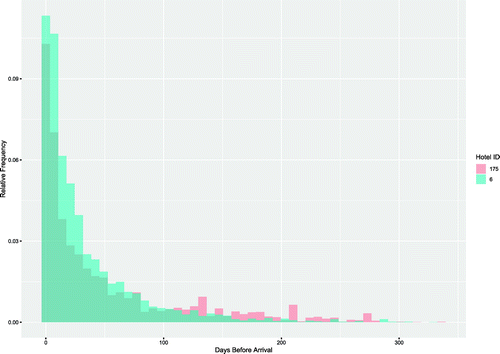
There is substantial dispersion in both the flow of bookings and the actual rates for the same room over time. Figure 1 shows the number of bookings as a function of days before arrival for the two largest hotels (IDs 6 and 175). Most bookings occur within 30 days of arrival, but there is a long right tail in each hotel. Given the booking pattern, it is not surprising that hotels change actual rates more often as the day of arrival approaches.7Table 2 summarizes the distribution of actual rate changes over the booking horizon of a product. Over the complete booking horizon, hoteliers change the actual rate of a product, on average, once a month. Because most bookings and price changes happen close to the arrival date, the median consumer can expect to see a price change every two weeks.8 Conditional on the actual rate changing, the median absolute adjustment amounts to about 8 euros per night.
|
Table 2. Actual Rate Updates over Time
| Room category | Days before arrival | |||
|---|---|---|---|---|
| 100–0 | 50–0 | 30–0 | 14–0 | |
| Single | 0.0251 | 0.0367 | 0.0444 | 0.0553 |
| Standard | 0.0465 | 0.0717 | 0.0918 | 0.1130 |
| Suite | 0.0189 | 0.0262 | 0.0322 | 0.0393 |
| Superior | 0.0347 | 0.0498 | 0.0616 | 0.0769 |
Notes. Fraction of days with an actual rate update by the hotel manager for different intervals of days before arrival. Data include only products for which we observe days before arrival.
2.2. Price Recommendations
A crucial input to our analysis are recommended rates provided by the revenue-management system. We are not aware of any other study that exploits price recommendations provided to managers to estimate demand. The RMS, which produces recommended rates for the hotel manager, works as follows. The revenue-management company offers an RMS service with the objective to maximize the client’s revenue through optimized pricing. It is incentivized to provide the best possible performance because the fee hotels pay for the service is benchmarked against expected revenue increases generated by the service. For price optimization, the revenue-management company has access to all bookings from a hotel on a real-time basis, as well as additional demand-related information, such as local variation in weather conditions, events, public holidays, hotel reputation, competitor prices, etc.
In addition, the revenue manager and the hoteliers are regularly exchanging information about local demand conditions. Clients are trained to transmit private information about local demand shocks to the revenue-management company. The company combines all relevant information and feeds it into their proprietary pricing algorithm to produce a rate recommendation for each product of the hotel.9 The hotelier decides every day whether to log into the system. If she does, she observes the current rate recommendation for each room and then decides which rates to update and by how much.10 After manual confirmation by the hotelier, updated actual rates are pushed from the RMS to the hotel’s property-management system and distribution channels (mostly OTAs).
Although the hotels in our data are typical for their respective regions, with about 50 rooms per hotel, they are relatively small by international standards. Most of them are family run, which means that the manager’s job description includes many responsibilities beyond revenue management. From private communications with the revenue-management company, we learned that managing prices takes only a small fraction of a hotelier’s weekly work schedule. In Section 3.4, we provide a detailed account of the behavioral response of hotel managers to rate recommendations. There, we show that hotel managers follow algorithmic recommendations quite closely, but do so with a delay. This will be an important ingredient of our identification approach.
3. Empirical Framework
A common challenge encountered in market studies is to find sources of exogenous variation in prices that allow us to identify demand. In our setting, the statistical inference problem is further complicated because we are interested in price variation over time for the same physical object. An instrument, therefore, should vary not only across arrival dates (e.g., shocks to capacity), but also across booking dates for a given arrival date, and these shocks should be unanticipated (e.g., news shocks about future costs). We circumvent this problem by leveraging rate recommendations, which allows us to isolate price changes that are plausibly uncorrelated with contemporaneous demand shocks.
3.1. Demand Estimation
In each booking period , with t = 0 representing the date of arrival, the manager at hotel h sets a price for product (e.g., a standard room for March 20) according to
The revenue manager forms recommendations according to
We assume that the number of bookings for a given product i that occur t days before arrival can be written as
(Exogeneity).
(Conditional Independence).
As shown later, we do not need to include the price in the exogeneity assumption because it is determined by the recommendation and observables. The second assumption is guaranteed, for instance, if νhit captures only variations in the availability of the hotelier to make changes in actual rates and local cost shocks, but does not include information about demand shocks. For this to hold, it is sufficient that any information that the hotelier obtains about demand is incorporated in the revenue-management system.12 It then follows that we can directly estimate the parameter ηh from
The last equality holds, because of the two identifying assumptions, the fact that is measurable with respect to and the identical equality , where fh is measurable.
In the empirical implementation of our framework in Section 4, we allow to vary across different room-type-arrival-month combinations, days before arrival t, and also across weekdays, in which hoteliers update rates. The latter variable allows us to pick up manager-specific variation—for example, arising from her schedule at work.13 Finally, notice that ηh in Equation (4) can be interpreted as the marginal impact of the price on the probability that a booking occurs on a given date. It can be thought of as an estimate of the derivative of the residual demand curve of a given product (hotel-room-type-arrival-date combination), which contains information about the responsiveness of consumers to a price change, as well as an implicit conduct parameter measuring market competitiveness. In Online Appendix EC.3, we extend our framework and study heterogeneity in price elasticities by allowing ηh to vary across different dimensions, such as booking weekdays and seasons of arrival (e.g., Puller and Taylor 2012; Semenova et al. 2021).
3.2. Generality of Empirical Framework
The above estimation approach is neither restricted to the particular institutional setting nor the pricing application we study empirically in this paper. It can be adapted to a variety of setups that use recommendation systems, or decision support systems (DSSs), more generally. The fundamental idea is to use plausibly exogenous variation in how recommendations are implemented behaviorally by decision makers to identify the marginal impact of the choice variable (e.g., prices) on the outcome variable (e.g., sales). In the following, we present two examples that fit well in our framework.
3.2.1. Staffing.
A number of papers have estimated the effect an additional worker has on profits by constructing a predictive model of staffing behavior and then exploiting observed departures from it as the exogenous variation in staff levels (e.g., Mani et al. 2015 and Fisher et al. 2020). Although such methods may work well in some cases, it is generally difficult to assess the extent to which the econometrician’s model is misspecified and the observed departures truly exogenous. Nevertheless, many organizations adjust their workforce at different locations based on their own demand predictions. This adjustment is rarely perfect because managerial inattention and worker availability can generate deviations from the ideal level of staff, given the predicted demand. Our framework can be directly applied to identify the marginal effect of an additional worker on sales if the realized number of workers does not perfectly match the firm’s own prediction of the optimal staffing level. To be more specific, let pit denote the staff level at location i at time t, and let the rest of the variables in Equation (1) be as before, with rit denoting the ideal level of staff given the predicted demand. Provided that there is some exogenous variation how the realized level of staff is determined, conditional on the ideal level, one may obtain a causal estimate of the marginal impact of a worker on sales by estimating the analogue of Equation (4).
3.2.2. Inventory Management.
One of the areas in which DSSs have been employed heavily is inventory management (e.g., Shang et al. 2008 and Van Donselaar et al. 2010). As above, let rit denote the restocking recommendation from the DSS and pit its realized flow. Our framework can be used to estimate the marginal effect of an additional stocked unit on sales. Holding excess inventory is costly, and, therefore, the causal impact of stock on revenue is a critical component of optimal inventory management.14 This can be directly identified by using the model described in Equation (4).
Finally, it is also illustrative to consider the limits of our framework. For example, consider a loan officer who has to assess the creditworthiness of a client with the help of a DSS. Suppose a researcher has data on these decisions and wants to estimate the marginal return of funds allocated to credit. In case the officer’s decision differs from the DSS’s recommendation because her decision is based on additional soft information about the client (Liberti and Mian 2008), rather than being a by-product of managerial inattention, then our critical assumption is violated, and our approach cannot be used. For this reason, we provide in Section 3.4 a wealth of evidence suggesting that managerial inattention is the main source of variation in our hotel sample.
3.3. Machine Learning and Model Selection
The recent literature on statistical inference with machine learning has shown that proper model selection can have important effects on estimated demand elasticities (e.g., Chernozhukov et al. 2015, Athey and Imbens 2019, and Dube et al. 2020). Applied to our setting, these insights mean that correctly selecting fh can be highly important for guaranteeing unbiased estimates of ηh. Especially if the revenue manager is not perfectly informed about the hotelier’s objective function, it becomes critical to correctly control for possible confounds. Even conditional on the revenue manager’s recommendations, there may remain demand-related confounds that are correlated with both the price and frequency of bookings. For example, a combination of fixed costs and credit constraints may lead the hotel manager to price more aggressively during the off-season to guarantee enough bookings to remain solvent. Consequently, the relationship between the actual rate and the recommended rate could vary in a way that is correlated with the intensity of demand, violating our identifying assumption.15
Furthermore, the response of the hotel manager to the price recommendation may depend both on its magnitude and its timing. Allowing for flexible controls for weekday-month combinations, the days before arrival, a third-order polynomial of the recommended prices and its interactions with both the weekday and arrival-month dummies already implies more than 500 potential parameters. When the median number of bookings in a hotel is less than 7,500, informative inference on the effect of price on demand while estimating all of these parameters is challenging. We solve this problem by applying the “post-double-selection” method from Belloni et al. (2014) to select the approximately right set of controls that leads to consistent estimates of the price elasticity of demand. We demonstrate in Online Appendix EC.2 that the nuisance parameter problem is indeed binding for simulated data sets comparable to the ones used in our application; in particular, estimates of the price semielasticity of the linear model are shown to be downward-biased.
For the application of the post-double-selection method, and with a slight abuse of notation, let J, with a typical element j, be the index set of possible controls, , that includes a flexible polynomial of the recommended price and its interactions with weekday and month-of-arrival dummies. As a first stage, we use a standard LASSO to estimate
The post-double-selection estimator for hotel h is then given by the least-squares estimator obtained by regressing Qhit on phit and the control terms selected in the previous stages, , with :
The vector γh contains the regularized regression coefficients for the control variables. Belloni et al. (2014) show the consistency and asymptotic normality of this estimator and also demonstrate that the standard errors for the last stage yield asymptotically correct confidence sets. They also provide an algorithm for estimating the penalty loadings for the two LASSOs in the selection stages.16
3.4. Validity of the Identifying Assumptions
In addition to controlling correctly for fh, identification relies on two behavioral assumptions on the relationship between the hotel manager and revenue manager. First, we assume that the price recommendation is a sufficient statistic for the information held by the revenue manager. Second, we assume that the variation in actual rates, conditional on observable product characteristics and recommended rates, is due to factors orthogonal to variation in demand. In addition to the information about the institutional relationship between the revenue manager and hotelier presented in Section 2, we present in this subsection evidence in support of these two identifying assumptions. To do so, we perform a deeper analysis of the recommendation data from the pricing algorithm, as well as the behavior of the hotelier, when making pricing decisions.
The first assumption can be recast as a communication game between the revenue manager and the hotel manager. In this game, the recommendation sent by the revenue manager is the message, and the actual rate is the action of the hotelier. If the incentives of the revenue manager are sufficiently aligned with those of the hotel manager, a truth-telling equilibrium, in which the recommendation is the best predictor for the current demand shock, exists.17 More realistically, however, incentives of the two contracting parties may not be perfectly aligned. In comparison with the hotelier, the revenue manager may, for instance, weigh revenue more heavily than profits and may not face negative consequences from excessive price variation. If this was the case, it would suffice that the revenue manager would suffer an additional reputational or moral cost if she distorted her recommendation excessively (see, e.g., Kartik 2009). This would allow for a monotone signaling equilibrium, and the invertibility assumption would still hold. In Online Appendix EC.2, we report on a simulated model in which recommendations are systematically biased; our estimates remain valid despite the bias.
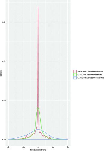
To further evaluate the role of price recommendations in the formation of actual rates, we construct a large LASSO prediction model, which does not include recommended rates, to predict the actual rates. We then compare the residuals from this model (i) to the same LASSO prediction model, which includes recommended rates as a predictor; and (ii) to the raw difference between the actual rates and the recommended rates. The resulting distributions of residuals from the three models are shown in Figure 3. Although observable characteristics clearly help in predicting the actual rate, the recommended rate alone does a much better job than our large LASSO model without recommended rates. The figure also shows that the LASSO predictions improve considerably when the recommended rate is added as a control. This improvement implies that the hotelier finds the revenue manager’s recommendations highly relevant when setting prices. Furthermore, the high frequency at which the price recommendation matches the actual rate demonstrates clearly that a hotel manager often copies the price recommended by the revenue manager perfectly. This strongly indicates that a hotel manager often follows the revenue manager’s advice.18
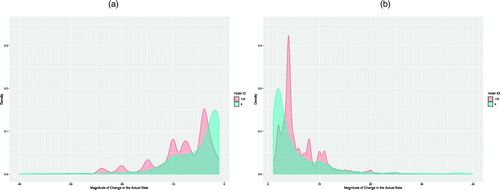
Notes. (a) Price decreases. (b) Price increases.
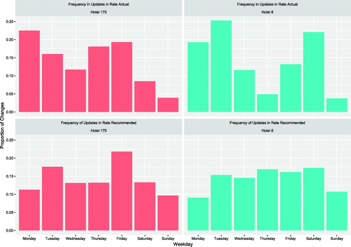
Regarding the second identifying assumption, we show that the residual variation in the difference between actual and recommended rates is unlikely to be related to variation in demand. To do so, we first consider the variation in the frequency of updates on different weekdays in both the actual rate and the recommended one. Figure 4 plots the distribution of rate updates in both the actual rate and the recommended rate for every day of the week in the two biggest hotels in our data (IDs 6 and 175). The distribution of updates in the actual rate has clear gaps that are likely related to the hotel manager’s workflow. For example, the manager of hotel 6 probably works on other things than pricing on Thursdays and Sundays and updates most frequently on Tuesdays and Saturdays. The recommendation updates are much more evenly distributed over the week, and their frequency does not seem to be related to the peaks in the hotelier’s distribution of rate updates. Similar patterns can be seen for all hotels in Table 3.
|
Table 3. Distribution of Actual Rate Updates
| Hotel ID | Monday | Tuesday | Wednesday | Thursday | Friday | Saturday | Sunday |
|---|---|---|---|---|---|---|---|
| 6 | 0.19 | 0.24 | 0.11 | 0.04 | 0.12 | 0.25 | 0.04 |
| 10 | 0.19 | 0.06 | 0.27 | 0.09 | 0.07 | 0.16 | 0.17 |
| 11 | 0.17 | 0.47 | 0.02 | 0.04 | 0.18 | 0.12 | 0.00 |
| 23 | 0.14 | 0.14 | 0.19 | 0.12 | 0.24 | 0.10 | 0.08 |
| 30 | 0.22 | 0.10 | 0.17 | 0.25 | 0.16 | 0.06 | 0.03 |
| 131 | 0.14 | 0.15 | 0.16 | 0.07 | 0.16 | 0.17 | 0.16 |
| 175 | 0.22 | 0.16 | 0.12 | 0.19 | 0.19 | 0.08 | 0.04 |
| 192 | 0.12 | 0.16 | 0.30 | 0.04 | 0.14 | 0.11 | 0.13 |
| 208 | 0.07 | 0.31 | 0.07 | 0.08 | 0.36 | 0.03 | 0.06 |
Notes. Numbers in bold indicate the day with maximal or minimal density of actual rate updates for each hotel. Rate updates for each hotel sum to one; rounding errors may apply. Data include only products for which we observe days before arrival.
Note that updating the prices for all arrival dates within the next two months in the median hotel requires one to manually update 300 different rates. It is, hence, reasonable for a hotel manager to economize on this dimension by concentrating the workload on certain weekdays. Observed updating behavior is also in line with the work schedule and responsibilities of hotel managers in our data given in Section 2 (see also endnote 18).
The timing and magnitude of deviations between the actual and recommended rates, conditional on an update, can be rationalized by standard models of price adjustment (see, e.g., Reis 2006 and Alvarez et al. 2011). In these models, managers have only partial information about demand and incur some observation cost for reassessing the optimal price. Managers trade off the benefits of a more precise price with these observation costs and choose to pay these costs only when the average expected update is sufficiently high. From this, it follows that the realized average update will be roughly independent of time. The posited behavior matches exactly the pattern we see in our data. The scatter plot in Figure 5 shows the magnitude of all rate updates as a function of time since the last update. The locally smooth best predictor of the magnitude of the price update as a function of days since the last update is roughly constant and is the same for price increases and decreases and across different hotels. Similarly, consistent with models with observation costs, the correlation between recommendations and prices is fairly constant over the booking horizon.19
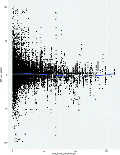
Notes. An observation corresponds to an update in the actual rate. The plotted line is the best locally smooth predictor of the average change as a function of days since last update.
3.4.1. Price-Setting Heuristics of Hotel Managers.
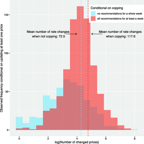
As a final piece of evidence, we show that part of the variation in prices is consistent with satisficing behavior by managers (Simon 1956).20 Hotel managers often resort to behavioral heuristics in room pricing because keeping a large number of prices up to date is a perpetual and daunting task. A particularly common behavior of hotel managers observed in our data is to accept all rate recommendations for a given room in a given week—that is, implement the recommended rate on every single night of the week. With approximately 22,000 such events in our data, they account for 52.2% of all rate updates by hotel managers. It is unlikely that these events are driven by private information of a hotel manager. Indeed, the data show that on days in which we observe a hotel manager “accepting all” recommendations for a room for a given arrival week, we typically also observe dozens of other unrelated rate updates, often for completely different arrival dates. This can be seen in Figure 6, where we plot the total number of actual rate changes (in log scale) on booking days when the hotelier copies all recommendations for at least one whole week and on booking days when none of the arrival weeks fully match the recommendation. It can be seen from Figure 6 that hoteliers adjust considerably more rates on days in which they copy recommendations. This indicates that following algorithmic recommendations is much less costly for the hotelier than coming up with a large number of optimal prices herself. We will present a number of difference-in-difference estimations in Section 4.1, which leverage the timing of these events, to obtain a credible quasiexperimental benchmark for our main specification.
To illustrate the weekly updating pattern of actual rates by hotel managers, we first run a simple regression (see column (1) in Table 4), which predicts changes in actual rates by changes in recommended rates and hotel-room type and arrival-month fixed effects. We group all observations from booking dates that share the same room type and the same arrival week; we refer to these observations as “peer” products. We then regress the residuals from the first regression on the average change in actual rates of other peer products, as well as the average change in prices of nonpeers with the same booking date. One would expect any private information about demand that is not already incorporated in the recommendation in the first stage to be correlated with demand for other products and, hence, induce a strong correlation between the nonpeer prices and the residual from the first stage. According to our results in column (2) in Table 4, a 1-euro increase in the prices of all peer products is associated with a 0.96-euro increase in the price of a given product, whereas a 1-euro increase in the prices of nonpeer products is associated with an increase of only 4 cents in the price of that same product. The adjusted R2 in the residual regression is 0.96. Together, these results imply that almost all of the residual variation in the actual rate is captured by the actual rate for that calendar week and room type. Hence, hotel managers update mostly rates for one calendar week at a time for a given room type, using similar adjustment heuristics for all arrival days in that week. At the same time, spillovers across arrival weeks and room types are marginal at best.
|
Table 4. Hotel Managers’ Updating Behavior and Product Similarity
| Variable | Dependent variable | |
|---|---|---|
| Δactual rate | Residual from column 1 | |
| Δrecommended rate | 0.936 | |
| (0.073) | ||
| Days before arrival | −0.005 | |
| (0.009) | ||
| Mean Δactual rate peers | 0.964 | |
| (0.013) | ||
| Mean Δactual rate nonpeers | 0.036 | |
| (0.013) | ||
| Hotel-room type FE | Yes | — |
| Arrival month FE | Yes | — |
| 0.26 | 0.96 | |
| N | 131,699 | 117,469 |
Notes. All regressions are estimated conditional on a change in the actual rate. A peer of a product is defined as a room in a hotel on a given arrival date that is otherwise identical to the product in question, but has its arrival date within a calendar week from the product being considered. For example, on the booking date January 2 for a double room in hotel 6 on the arrival date of June 1 (Thursday), the mean Δactual rate peers would be the average change in actual rate between January 1 and January 2 for double rooms in hotel 6 for all arrival dates in May 29 (Monday) through May 31 (Wednesday) and June 2 (Friday) through June 4 (Sunday). The difference in the number of observations between columns (1) and (2) is due to some products having no peers or all of the remaining observations being its peers. Standard errors clustered at the hotel level. FE, fixed effects.
***.
4. Empirical Results
Based on our demand-estimation framework, we now report results from various specifications of the following model:
In this model, the dependent variable Qhit equals one if there is a booking for a room-type-arrival-date combination, or product, i (e.g., standard room for March 21) at hotel h, t days before arrival. The average probability of a booking on a given day is 2.4%, and only very rarely do we observe multiple customers purchasing the same room-type-arrival-date combination on the same booking date. The main regressors are the actual rate, or price, phit, and the rate recommended by the revenue manager rhit. We allow the recommended rate to have a nonlinear impact on the actual rate and allow for different hotels to adjust rates differently. We allow the LASSO to pick from a set of controls that includes month- and weekday-of-arrival fixed effects, their interactions with a third-order polynomial of the recommended rate, booking horizon fixed effects, and all interactions between the month of arrival and the weekday of arrival. The strength of the double-selection method is that it allows for highly flexible forms of the potentially infinite dimensional “nuisance parameter” fh with a finite amount of data while still delivering consistent estimates of ηh.
We start by estimating the relationship between actual rates and daily bookings using a double-selection (DS) procedure in which recommended rates are completely omitted. The results are summarized in column (2) in Table 5, where we report the seventh (L), fifth (M), and third (H) highest semielasticities out of our nine hotels. Omitting recommended rates yields often positive or very small coefficients of price on quantity, suggesting endogeneity, despite the large number of seasonal controls. Even those hotels for which we would estimate negative price elasticities would be able to charge markups ranging from 100% to 200% of their price—that is, implying prices inconsistent with profit maximization. We then consider a simple fully linear specification without double selection, where we include only actual rates, recommended rates, and room-type fixed effects on the right-hand side. The results can be found in column (1) of Table 5. More hotels now exhibit a negative relation between price and quantity, but there is still huge dispersion across hotels.21
|
Table 5. Demand Semielasticities in p.p.
| Variable | Model specification | ||||
|---|---|---|---|---|---|
| Simple OLS | DS linear | DS linear | DS log-log | DS logit | |
| Actual rate (L) | 0.23 | 0.04 | 0.05 | ||
| Actual rate (M) | −0.15 | −0.29 | |||
| Actual rate (H) | |||||
| Recommended rate | Yes | No | Yes | Yes | Yes |
Notes. The dependent variable is the probability of a booking for a given product on a given date. We run a separate regression for each hotel. The ordinary least-squares (OLS) results control for room type and recommended price. DS in columns (2)–(5) refers to double-selected models. In columns (3)–(5), the double-selection method is allowed to select from a third-order polynomial of the recommended rate and its interactions with the month of arrival and weekday of booking, room type, interactions between the weekday of arrival and arrival month, and indicators for the number of days before arrival. In column (2), the set of controls is the same, but does not include the recommended rate or any of its interactions. Reported coefficients correspond to the third (H), fifth (M), and seventh (L) most elastic estimate out of the nine hotels. The semielasticities for the logit model in the last column are calculated by using the average marginal effect of a price change divided by the average booking rate. Standard errors are in parentheses.
**; ***.
Next, we run a double-selection regression in which we include the same large set of potential controls, as in column (2) of Table 5, including a flexible polynomial of the recommended rate and interactions between seasonal characteristics and recommendations. These interactions capture the (possibly) nonlinear response of hotels to information and are consistent with the model described in the previous section. Results from this (preferred) specification are summarized in column (3).22 The median hotel faces a 1% drop in bookings should they increase their price by 3 euros. Translated into markups, these estimates suggest that the median hotel’s variable profit from an additional purchase is approximately 55% of its price.23 This median masks substantial variation across hotels. For example, hotels 175 and 6 are facing much more elastic residual demand functions, as we show below. Similar results are obtained by using both a log-log and a logit specification (see columns (4) and (5) in Table 5). The first allows for the baseline arrival rate to affect demand multiplicatively rather than additively, while the second appropriately handles the large number of days with zero bookings in our data set.
Leveraging the richness of our data, we can also compute hotel-room-type-specific semielasticities. For each hotel, we estimate the following model:
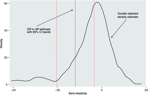
Notes. Kernel-density plot (Epanechnikov kernel with bandwidth = 0.0027) of the estimated semielasticities across all room types and hotels using double selection (Table 5) is shown. Although kernel-density estimates exhibit some mass at positive values, only three estimates are statistically larger than zero. The figure also plots the difference-in-differences estimate reported in Table 6. The vertical line represents the difference-in-differences (diff-in-diff) estimate, and the dashed lines the corresponding 95% confidence intervals.
For more advanced dynamic pricing features, we can also investigate heterogeneity in price elasticities beyond the hotel-room type (see also Semenova et al. 2021). As an illustration, we provide in Online Appendix EC.3 price elasticity estimates for different booking days of the week, as well as arrival seasons, which may both depend on the type of consumer—for example, holiday or business traveler—a hotel faces.
4.1. Difference-in-Differences Estimations Using Accept-All Events
An alternative, more direct approach to exploit the variation in our data is to run a simple difference-in-differences estimation. To this end, we restrict our analysis to accept-all events—that is, events in which a hotelier updates all rates for a given week and room type by following the recommendation perfectly. We restrict our data to two-day windows around these events, observing the prices and demand before and after the event. As the hotelier is exactly matching the recommended rate for a whole week of arrival dates, these events are unlikely to be driven by new information and should, rather, be interpreted as a useful behavioral heuristic that busy managers fall back on when updating rates. In particular, our identification assumption is that the exact timing of the actual rate update is uncorrelated with contemporaneous, hotel-specific demand shocks within the two-day window. Because the recommendation was already in place on the first day, it is natural to assume that, had the manager decided to make a change for this particular week the day before, she would have chosen the same actual rate. In other words, the difference between the two rates was due to managerial inattention. This arguably quasiexperimental variation allows us to apply a difference-in-differences logic comparing demand and actual rate changes over those two days, using similar rooms in other hotels without an accept-all event on that same day for the same arrival week as the control group.
Denote by Δ the first-difference operator on a given variable, such that . Let δhit be a dummy variable that takes the value one if hotel h has an accept-all event on date t for room i. Our regression equation is
Table 6 summarizes the results. The estimated coefficient for the change in price across consecutive days, θ, is very small and statistically insignificant. In particular, the coefficient corresponds to an implausibly low semielasticity of –0.045 percentage points (p.p.) and is very precisely estimated (standard error 0.05). That is, we find no significant correlation between changes in actual rates and contemporaneous quantity changes at the product level for those price changes that do not exactly match the recommendation. Instead, we find a sizeable and statistically significant effect of the interaction term: The estimated coefficient of the difference-in-differences equation, η, translates into a semielasticity of –1.2 p.p., and we cannot reject the null hypothesis that the estimated coefficient equals the estimated semielasticity for the median room (see Figure 7).
|
Table 6. Estimates of the Slope of the Demand Curve and Implied Demand Semielasticities in p.p. from the Difference-in-Differences Specification
| Variable | Model specification | |||
|---|---|---|---|---|
| All observations | Excl. suites | Last 20 days | Excl. last 20 days | |
| Δactual rate | −0.0018 | −0.0027 | −0.0044 | −0.0012 |
| Δactual rate × copied all recs | ||||
| Copied all recommendations | −0.145 | |||
| Average booking rate | 0.038 | 0.041 | 0.077 | 0.019 |
| Semielasticity in p.p. (interaction) | −1.20 | −1.22 | −0.88 | −2.22 |
| Product category – time FE | Yes | Yes | Yes | Yes |
| N | 5,886,196 | 4,603,198 | 631,864 | 5,254,332 |
Notes. The dependent variable is the change in the number of a bookings (in p.p.). Copied all recommendations equals one if on that booking day, the hotel manager updated at least one price, and all of the prices for that arrival week matched the recommendation. Note that this requires matching prices also for other room types. Fixed effects (FE) are at the level of unique combinations of room category, date of arrival, and booking date. Standard errors shown in parentheses are clustered at the hotel level. Excl., excluding.
**; ***.
The treatment group for the difference-in-differences regression above requires that the hotel manager update rates for a full week of arrival dates for a given room type and match the recommended price while doing so. A natural question here is whether the event of updating a full week of prices for the same room type will introduce enough exogenous variation in the prices in the form of pricing mistakes and delays to yield reasonable estimates, even if price recommendations are unavailable. When we run the same model as in the first column of Table 6, but do not require that all prices in the treatment group match the recommendation after the price change, the estimated elasticity becomes positive (the estimated coefficient is 0.045 with a standard error equal to 0.025). We conclude that a sizable number of simultaneous prices changes, without controlling for the recommended prices, is not enough to control for the endogeneity resulting from hotel manager’s information about demand shocks.
The lack of power of the above difference-in-difference approach using accept-all events might seem surprising at first, especially because there are 819 hotel-booking-day pairs on which the hotel manager copied the recommendation for a whole week. However, given the low average booking rate, very few of the day pairs around the copying event have contemporaneous bookings, explaining the low power (see also simulation results in Online Appendix EC.2). As the variation in prices in this model is very likely to be exogenous, we think that the results presented here serve as an excellent test for whether the estimates from the double-selected model in the previous section are close to the truth.
The direct applicability of this difference-in-differences approach in real-world applications is, however, quite limited, as the method requires data sets with very large numbers of bookings and cannot be applied at the hotel level, at least for the medium-sized hotels in our sample (because our hotel-level estimates exhibit considerable heterogeneity). Furthermore, the difference-in-differences approach provides only a local average treatment effect around the days the hotel manager copied recommendations. If the sporadic updating behavior is driven by adjustment costs, hotel managers are adjusting prices more frequently when the payoff from doing so is high. Consequently, such estimates are going to be applicable only in times of relatively high demand. Lastly, the difference-in-difference model requires panel data, whereas our control-function approach can be applied to cross-sectional data as well.
4.2. Why Standard Instrumental Variables Do Not Work
The classical approach to demand estimation involves the use of instrumental variables. Roughly speaking, three types of instruments have been used in the literature: cost shifters, characteristics of other products, and prices in other markets (Hausman instruments). In the hotel industry, there are no obvious cost shifters that move frequently enough to help identify demand when firms engage in dynamic pricing. Similarly, characteristics of other competing hotel rooms vary only over the very long run and, thus, cannot be used as instruments for these types of data sets. The only remaining potential candidate is to leverage prices in other markets to capture supply shocks. The key identifying assumption is that, conditional on product characteristics, the contemporaneous demand shock of hotels h and are uncorrelated if they are located in different markets. This assumption is likely to hold in markets where demand is driven by income shocks or taste parameters, but perhaps less likely to hold in the hotel industry. In particular, weather shocks are strongly correlated across local markets.
To investigate the performance of this instrumental variable (IV) approach, we use the “triple selection” IV algorithm from Chernozhukov et al. (2015), in which we include as instruments prices of hotels located in other regional markets. The algorithm allows us to select both the relevant exogenous controls and instruments. In particular, we estimate
Table 7 shows that the above IV model yields mostly positive and highly heterogeneous coefficients. This suggests that the instruments are endogenous or, put differently, that the identifying assumption of demand shocks for hotels in different markets does not hold. The endogeneity is so strong that the estimates are biased, even when controlling for recommended rates.
|
Table 7. Triple-Selected Instrumental-Variable Regressions
| Variable | Set of instruments and booking horizon | |||
|---|---|---|---|---|
| All | Only hotel 6 | All excluding last 15 days | ||
| Actual rate (L) | ||||
| Actual rate (M) | 0.05 | 0.001 | ||
| Actual rate (H) | −0.025 | 0.01 | ||
| Recommended rate | Yes | Yes | No | Yes |
| Hotel ID | All | Six excluded | 175 | 175 |
Notes. The dependent variable is the number of bookings for a given product on a given date. All specifications use the three-step selection procedure introduced in the main text. We run a separate regression for each hotel. Reported coefficients correspond to the third (H), fifth (M), and seventh (L) most elastic estimate out of the nine hotels. Control variables include month and day of arrival and room-type indicators and days before arrival. In columns (1), (2), and (4), the triple-selection method is allowed to select from a third-order polynomial of the recommended rate and its interactions with the month of arrival and weekday of booking, room type, and fixed effects for days until arrival. Instruments are prices in other hotels. In column (2), we only use prices in hotel 6 as instrument, and we drop hotel 6 from the main analysis. In columns (3) and (4), we exclude the last 15 days. Standard errors are in parentheses.
*; ***.
One might argue that the main driver of correlation in demand shocks across hotels in our application is weather. Because weather forecasts are not very reliable more than 15 days ahead, excluding the last 15 days before arrival would remove any endogeneity resulting from common weather shocks. Results from the IV model, excluding the last 15 days before arrival, are reported in the last two columns of Table 7. Only if we include recommended rates as a control, the IV regression is able to identify a negative price coefficient (see column (4)). This illustrates that price recommendations contain information about common demand shocks that are not only restricted to local weather shocks. Overall, we conclude that Hausman-type instruments are unlikely to provide credible estimates due to unobserved and correlated demand shocks in the hotel industry.
5. Applications: Dynamic Components of Demand
We now demonstrate our empirical framework by investigating two essential features of demand in the hospitality industry. First, we perform a heterogeneity analysis by studying variation in price sensitivity of consumers across different time horizons, which is crucial for intertemporal price discrimination. Second, we introduce lagged prices in our main regression framework to investigate whether, and to which extent, current demand is affected by previous price changes. The idea is that if some consumers would be willing to delay their purchase in the hope of a better price in the future, lagged prices would be positively correlated with current demand.
5.1. Time-Varying Price Elasticities
Williams (2022) shows in an application of dynamic pricing in the airline industry that the benefits of intertemporal price discrimination depend crucially on the temporal pattern of consumers’ price sensitivity. Because the average opportunity cost (conditional on not having sold the room) is decreasing over time, the optimal price should fall, as long as the semielasticity of demand remains constant. To investigate intertemporal price sensitivity of customers for our hotel data set, we run our double-selected baseline specification for two hotels (6 and 175) separately for different booking horizons.25 Results suggest that the estimated price semielasticity is highest for early bookings and lowest for late bookings, as shown in Table 8. Our results are consistent with the intuition that consumers who search early on are relatively more price-sensitive. This finding contrasts with recent work by Joo et al. (2020), who find that the price sensitivity increases over time for holiday cruises.
|
Table 8. Double-Selected Demand Semielasticities in p.p. over Time
| Hotel | Days before arrival | |||
|---|---|---|---|---|
| Hotel 6 | −0.31 | |||
| (0.58) | (0.58) | (0.56) | (0.34) | |
| Hotel 175 | ||||
| (0.21) | (0.23) | (0.19) | (0.12) | |
Notes. The dependent variable is the probability of a booking in hotels 175 or 6 for a given product on a given date. Control variables that the double selection is allowed to select from include month and weekday of arrival, room-type indicators, a third-order polynomial of the recommended rate and its interactions with the month and weekday of arrival, interactions between the weekday of booking and arrival month, and indicators for the number of days before arrival. Actual rate is the rate on the day of booking. Lagged rate is the rate eight days before the booking. We run separate regressions for each hotel and each booking horizon. Standard errors are in parentheses.
**; ***.
We can also use these results to decompose the observed price into the markup and the opportunity cost (containing both marginal operating costs and foregone future opportunities), disregarding potential cross-substitution patterns across products and forward-looking consumers. This decomposition is depicted in Figure 8. Prices in hotel 6 are remarkably constant over time, whereas for hotel 175, prices are increasing slightly with the arrival day approaching. Because opportunity costs fall over time, this pattern is prima facie inconsistent with profit maximization. Constant prices can only be rationalized if hotel 6 faces a decreasing price elasticity over time, which is what we find: Our estimated price elasticity is decreasing, and the implied optimal markups are increasing; see the dashed line of hotel 6 in Figure 8. This suggests that properly accounting for demand heterogeneity, such as temporal differences in demand of consumers, is key for dynamic pricing policies in our setting.

Note. Bookings 21–50 days before arrival for hotel 6 are excluded due to imprecise estimates (Table 8, column (4)).
5.2. Forward-Looking Consumers
Suppose that some consumers are willing to delay their purchasing decision and instead continue searching for a better price. We refer to these consumers as strategic, whereas the rest of consumers are assumed to be myopic. Strategic consumers, who delay their purchase waiting for better future prices, introduce a dynamic component in demand. Previous prices now have an impact on the probability that a strategic consumer who considered purchasing in the past remains active in the market.
More precisely, a price hike in the past has two distinct effects on the current demand of strategic consumers, as we show in the online appendix (section EC.1). First, an increase in the price leads some consumers to strategically delay purchases in the hopes of obtaining a better price in the future. Second, some consumers who would have otherwise waited will exit the market in response to a price hike. The second effect is relatively important in our setting because prices seem to follow a martingale, in the sense that the best predictor for tomorrow’s price is today’s price (unless one has access to price recommendations).26 We refer to the sum of these two opposing mechanisms as the “market-size effect” of a price hike. Empirically, we consider the following model:
Results from the double-selection model for hotels 175 and 6 are summarized in column (2) of Table 9. We find that there is a persistent negative effect of lagged prices on contemporaneous demand for hotel 175, whereas this effect is positive for hotel 6. The magnitude of these effects is slightly bigger than half of the effect of contemporaneous prices, suggesting that the proportion of customers willing to delay purchases is substantial for both. Taken at face value, these results suggest that there exists significant heterogeneity in the response of customers to price changes across different hotels in our sample.
|
Table 9. Double-Selected Demand Semielasticities in p.p. Including Lagged Prices
| Variable | Model specification | ||
|---|---|---|---|
| Baseline | Incl. 8-day lags | Incl. interactions | |
| Hotel 175 (N = 827, 797) | |||
| Actual rate | |||
| Lagged rate | |||
| Actual rate × hike | |||
| Actual rate × drop | |||
| Hotel 6 (N = 204, 635) | |||
| Actual rate | |||
| Lagged rate | |||
| Actual rate × hike | 0.13 | ||
| Actual rate × drop | |||
Notes. The dependent variable is the probability of a booking for a given product on a given date. Control variables that the double selection is allowed to select from include month and weekday of arrival, room-type indicators, a third-order polynomial of the recommended rate and its interactions with the month and weekday of arrival, interactions between the weekday of booking and arrival month, and indicators for the number of days before arrival. Actual rate is the rate on the day of booking. Lagged rate is the rate eight days before the booking. Hike (drop) equals one if the current price exceeds (is lower than) the lagged price. Standard errors are in parentheses. Incl., including.
**; ***.
In addition, price changes in the past are known to change the composition of potential customers (Li et al. 2014). When prices are increasing (decreasing), the fraction of consumers who wait for future price reductions is smaller (larger, respectively). Consequently, the price elasticity depends mostly on the behavior of myopic consumers when prices are increasing and on strategic consumers when they are decreasing. To quantify these effects, we run the model described in Equation (8) interacting the actual rate with an indicator variable that equals one if the actual rates has increased and zero otherwise. Formally, restricting the sample to periods in which for , we estimate
6. Conclusion
Recommendation systems that support pricing, inventory, and production decisions are becoming ubiquitous with the rise of machine learning and artificial intelligence. In this paper, we have provided a novel approach leveraging historical recommendation data to isolate exogenous variation in pricing decisions that can be used in static as well as dynamic settings. Our approach credibly identifies the causal impact a price change has on demand, as long as algorithmic price recommendations are not perfectly passed on to final prices. It also allows for counterfactual analysis in environments where such inference was not possible with traditional methods, such as instrumental variable approaches.
Applying our general framework to pricing in the hotel industry, we provide evidence that hotel managers seem to face significant fixed costs for adjusting actual rates. Consequently, they integrate the information contained in price recommendations sluggishly and only partially into realized prices. We then show how the discrepancies between the recommendations and realized prices can be used to identify hotel- and room-type-level demand elasticities. Our paper adds to the empirical literature on dynamic pricing also because we can leverage our high-frequency pricing and booking data to identify a subset of the data that exhibits quasiexperimental variation in prices. A simple difference-in-differences estimation applied to this subset validates our more general hotel-level estimates.
Our method can be used to measure dynamic patterns in demand that have critical implications for optimal pricing. In our application to hotel pricing, we have provided evidence for strategic behavior by a significant fraction of consumers and established the existence of substantial heterogeneity in the price sensitivity of the average consumer as a function of the number of days before arrival. In comparison with structural models, our reduced-form approach can be easily adapted to account for the dependence of the price elasticity on other variables by estimating the interactions between the variable of interest and prices. A typical example is estimating cross-price elasticities for substitutes. Note that we have not included cross-price effects of substitute products for the elasticity estimations in the main text because they seem negligible in our application (see Online Appendix EC.4 for details). For other applications, however, extending the estimation approach and the underlying identification strategy to incorporate cross-price elasticities more generally would be a valuable exercise, which we leave for future research.
Finally, our approach only requires transaction-level data and, thus, represents an inexpensive alternative to both structural modeling and price experimentation, which are often outside the reach of all but the largest and technologically most advanced corporations. It extends easily to many environments in which managers face a large number of small decisions, daily prices in our setting, and have access to algorithmic recommendations.
The authors thank the corporate sponsor for making the data available for this project. The authors are particularly grateful to Hannes Ullrich, three anonymous referees, the department editor, and the associate editor for very helpful comments. The authors also thank audiences at the University of Vienna, the 2018 CESifo Network Conference on the Economics of Digitization, and the 2019 Industrial Organization Ausschuss for comments. William Burton provided excellent research assistance. The computational results presented have been computed in part by using the Vienna Scientific Cluster.
1 According to Eurostat statistics (https://ec.europa.eu/eurostat/), European Union 27 citizens spent in 2018 about 124 billion euros, or 1.7% of their total consumption expenditures, on accommodation services.
2 Exogenous, behavioral delays in the time it takes a manager to follow a recommendation to restock their wares can be used to estimate the marginal effect of an extra unit of stock on the probability of running out of stock. As long as stock-outs are relatively short and demand continuous overtime, lost demand during a stock-out can be estimated by using the number of units sold before and after the stock-out. Alternatively, one can also use sales data from similar stores that did not run out of stock.
3 There are a number of important differences between hotel-room and airline pricing with regards to strategic consumer behavior. Hotels, for instance, rarely use markdowns to price-discriminate across consumers based on the time of the day or the day of the week in which consumers search. From an applied revenue-management perspective, our empirical applications provide useful insights for optimal pricing in the hotel industry.
4 Li et al. (2018) is the only paper, other than the present article, to obtain credible estimates of dynamic demand for hotels using reduced-form methods. Reduced-form methods are undoubtedly more useful for practitioners. Indeed, both Cho et al. (2018) and Li et al. (2014) acknowledge that they use structural methods because in their applications, reduced-form estimates are likely to be contaminated by unobserved demand shocks.
5 Various strategies have been proposed recently to accommodate strategic behavior by consumers in the theoretical literature. Some models study how frequent discounts (Cachon and Feldman 2015) or randomized pricing policies (Chen et al. 2021) can counteract strategic behavior of customers. There are also a number of recent articles in operations research that complement the literature by providing novel robust approaches to dynamic pricing with strategic consumers (e.g., Besbes and Lobel 2015, Caldentey et al. 2016, and Chen and Farias 2018).
6 The total price paid can include, on top of channel-specific discounts, promotional discounts (e.g. “book x nights but pay only x − 1”), as well as extra charges (e.g., for room service or spa packages). As shown in Table 1, the average total price paid by customers is a relatively stable share of the average actual price of a product. For details on prominent distribution channels, specific discounts, and contractual settings relevant in the hotel industry, see, for example, Hunold et al. (2018), who study the effects of best-price clauses previously used by some online travel agencies (OTAs). Note also that rooms that are sold through long-term contracts between the hotel and a reseller, who may be free to set their own prices, are not included in the data.
7 The majority of transactions of a hotel are realized through online travel agencies or through a hotel’s website, but we do not have information about the specific booking channel used in a transaction. As mentioned above, we do not consider prices for specific booking channels in our analysis to estimate demand because we have direct access to actual rates.
8 This calculation assumes that the arrival of potential customers is proportionate to the number of bookings. In contrast to the setting in Li et al. (2014), in which strategic consumers can predict the direction of the price change of airline tickets, it is extremely difficult for the average potential customer to predict the direction or the magnitude of a change in the price of a product in our setting without observing the recommendation. Rate updates are not serially correlated, and they are fairly symmetrically distributed (see Figure 2).
9 We do not have access to the company’s proprietary pricing algorithm. A common concern in competition policy is that algorithmic pricing can be used to coordinate with competitors (Miklós-Thal and Tucker 2019). We believe that coordination through algorithmic pricing is not much of a concern in our context. Given the highly fragmented nature of the industry, the number of hotels that use recommendations from our corporate sponsor is very small () compared with the size of the industry in the considered regions.
10 In addition to recommended rates, the hotelier has also access to additional information on the RMS platform, such as prices of local competitors, own performance metrics, etc.
11 In our empirical analysis (see Section 4), we also include a model with a multiplicative structure.
12 See Section 3.4 for a more detailed discussion of the validity of the identifying assumptions.
13 An alternative specification would be a control-function approach, using a two-step estimation method (price on recommendation and controls and quantity on these residuals). In our case, however, this is not necessary because we can confidently rule out any direct effect of the recommendation on demand.
14 See Conlon and Mortimer (2013) and Cachon et al. (2019) for recent work on the same question.
15 Using a simulated data set, we provide in Online Appendix EC.2 evidence that the estimates from a simple linear model are severely biased.
16 In terms of computational resources, the complete estimation procedure took more than 8,000 CPU hours for the data set, including all nine hotels (using nine supercomputing nodes, each containing 256 GB of memory and two INTEL Xeon processors).
17 For instance, in Crawford and Sobel (1982), as the bias of the sender converges to zero, the most informative equilibrium becomes perfectly informative.
18 A cursory inspection of Figure 3 might lead to the conclusion that the recommended rate is doing a better job at predicting the actual rate than the LASSO that includes the recommended rate. This, of course, is not possible. The LASSO prediction has much less mass on the absolute errors in the 15- to 30-euro range. In terms of mean squared error, these mistakes are much more expensive than the errors in the 5- to 10-euro ranges, where the LASSO has considerably more mass than the simple recommended rate. Notice, however, that the LASSO that does not include the recommendation has more mass on all but the smallest errors than either of the two other predictions and, hence, performs considerably worse than them.
19 The idea of fixed costs for adjustment, as well as the use of heuristics in price setting, have a long tradition in economics and management.
20 Simon (1962, p. 10) argued that “…price setting involves an enormous burden of information gathering and computation that precludes the use of any but simple rules of thumb as guiding principles. Through detailed study of pricing by multiple interviews throughout the firm we begin to get a picture of the informational and computational constraints that hedge in the pricing process and give it form.”
21 This is consistent with the results from the simulated model, where ordinary least-squares estimates are biased in the presence of sufficiently many confounders; see Online Appendix EC.2.
22 We experimented with a version of this model that includes an even larger set of potential fixed effects and that is estimated by using the method suggested in Kock and Tang (2019). The results are quantitatively comparable and available from the authors on request.
23 The hotel’s variable profits are given by , where p is the price, q is the quantity sold as a function of price, and c is the marginal cost. The first-order condition for optimizing this with respect to the price can be written as , where is the semielasticity of demand, which, according to our preferred model, equals approximately –0.0038. The average expenditure, p, is approximately 477 euros. These computations disregard cross-price effects that multiproduct firms, such as these hotels, may want to take into account in their pricing; see Section 6 and Online Appendix EC.4 for more details.
24 This number is computed by simply performing the Taylor approximation of the profit function around the optimal price . Using our linear demand estimates, the average loss per room is Because , multiplying by the number of rooms yields a loss of about 40 euros.
25 Specifically, we distinguish between very early bookings (>100 days ahead), early bookings ( days ahead), late bookings ( days ahead), and very late bookings ( days ahead).
26 Intuitively, this can be seen from Figure 2, which plots the distribution of changes in actual rates. Price hikes and markdowns are distributed similarly, and the median change in either direction is 8 euros per night or 22 euros on an average booking; see also Figure 8.
References
- (2011) Optimal price setting with observation and menu costs. Quart. J. Econom. 126(4):1909–1960.Crossref, Google Scholar
- (2017) Beyond prediction: Using big data for policy problems. Science 355(6324):483–485.Crossref, Google Scholar
- (2019) Machine learning methods that economists should know about. Annu. Rev. Econom. 11:685–725.Crossref, Google Scholar
- (2015) Machine learning methods for demand estimation. Amer. Econom. Rev. 105(5):481–485.Crossref, Google Scholar
- (2014) Inference on treatment effects after selection among high-dimensional controls. Rev. Econom. Stud. 81(2):608–650.Crossref, Google Scholar
- (2016) Post-selection inference for generalized linear models with many controls. J. Bus. Econom. Statist. 34(4):606–619.Crossref, Google Scholar
- (2015) Intertemporal price discrimination: Structure and computation of optimal policies. Management Sci. 61(1):92–110.Link, Google Scholar
- (2015) Price commitments with strategic consumers: Why it can be optimal to discount more frequently… than optimal. Manufacturing Service Oper. Management 17(3):399–410.Link, Google Scholar
- (2019) Does adding inventory increase sales? Evidence of a scarcity effect in US automobile dealerships. Management Sci. 65(4):1469–1485.Link, Google Scholar
- (2016) Intertemporal pricing under minimax regret. Oper. Res. 65(1):104–129.Link, Google Scholar
- (2019) Who benefits from surge pricing? Working paper, Stanford University, Stanford, CA.Google Scholar
- (2018) Robust dynamic pricing with strategic customers. Math. Oper. Res. 43(4):1119–1142. Link, Google Scholar
- (2021) Intertemporal price discrimination via randomized promotions. Preprint, revised December 20, https://papers.ssrn.com/sol3/papers.cfm?abstract_id=3223844.Google Scholar
- (2015) Valid post-selection and post-regularization inference: An elementary, general approach. Annu. Rev. Econom. 7(1):649–688. Crossref, Google Scholar
- (2018) Optimal dynamic hotel pricing. Working paper, Seoul National University, Seoul.Google Scholar
- (2016) Using big data to estimate consumer surplus: The case of Uber. NBER Working Paper 22627, National Bureau of Economic Research, Cambridge, MA. Google Scholar
- (2013) Demand estimation under incomplete product availability. Amer. Econom. J. Microeconom. 5(4):1–30.Crossref, Google Scholar
- (2020) Machine + man: A field experiment on the role of discretion in augmenting AI-based lending models. J. Accounting Econom. 70(2-3):101360.Crossref, Google Scholar
- (1982) Strategic information transmission. Econometrica 50(6):1431–1451.Crossref, Google Scholar
- (2020) Monopsony in online labor markets. Amer. Econom. Rev. Insights 2(1):33–46.Crossref, Google Scholar
- (2010)
Competitive pricing in European hotels . Chen JS, ed. Advances in Hospitality and Leisure (Emerald Group Publishing Limited, Bingley, UK), 3–25.Crossref, Google Scholar - Fisher M, Gallino S, Netessine S (2020) Setting retail staffing levels: A methodology validated with implementation. Manufacturing Service Oper. Management 23(6):1562–1579.Google Scholar
- (2018) Evaluation of best price clauses in online hotel bookings. Internat. J. Indust. Organ. 61:542–571.Crossref, Google Scholar
- (2020) Temporal distance and price responsiveness: Empirical investigation of the cruise industry. Management Sci. 66(11):5362–5388.Link, Google Scholar
- (2009) Strategic communication with lying costs. Rev. Econom. Stud. 76(4):1359–1395. Crossref, Google Scholar
- (2019) Uniform inference in high-dimensional dynamic panel data models with approximately sparse fixed effects. Econometric Theory 35(2):295–359.Crossref, Google Scholar
- (2013) The welfare effects of intertemporal price discrimination: An empirical analysis of airline pricing in US monopoly markets. Working paper, New York University, New York.Google Scholar
- (2014) Are consumers strategic? Structural estimation from the air-travel industry. Management Sci. 60(9):2114–2137. Link, Google Scholar
- (2018) Price to compete…with many: How to identify price competition in high-dimensional space. Management Sci. 64(9):4118–4136.Link, Google Scholar
- (2008) Estimating the effect of hierarchies on information use. Rev. Financial Stud. 22(10):4057–4090.Crossref, Google Scholar
- (2015) Estimating the impact of understaffing on sales and profitability in retail stores. Production Oper. Management 24(2):201–218.Crossref, Google Scholar
- (2019) Collusion by algorithm: Does better demand prediction facilitate coordination between sellers? Management Sci. 65(4):1552–1561.Link, Google Scholar
- (2018) Randomized markdowns and online monitoring. Management Sci. 64(3):1271–1290.Link, Google Scholar
- (2019) Dynamic learning and pricing with model misspecification. Management Sci. 65(11):4980–5000.Link, Google Scholar
- (2005) Pricing and Revenue Optimization (Stanford University Press, Stanford, CA).Crossref, Google Scholar
- (2012) Price discrimination by day-of-week of purchase: Evidence from the US airline industry. J. Econom. Behav. Organ. 84(3):801–812.Crossref, Google Scholar
- (2006) Inattentive producers. Rev. Econom. Stud. 73(3):793–821. Crossref, Google Scholar
- (2021) Estimation and inference on heterogeneous treatment effects in high-dimensional dynamic panels. Preprint, revised March 16, https://arxiv.org/abs/1712.09988.Google Scholar
- (2008) A decision support system for managing inventory at GlaxoSmithKline. Decision Support Systems 46(1):1–13. Crossref, Google Scholar
- (1956) Rational choice and the structure of the environment. Psych. Rev. 63(2):129–138.Crossref, Google Scholar
- (1962) New developments in the theory of the firm. Amer. Econom. Rev. 52(2):1–15.Google Scholar
- (2004) The Theory and Practice of Revenue Management (Springer, Boston).Crossref, Google Scholar
- (2010) Ordering behavior in retail stores and implications for automated replenishment. Management Sci. 56(5):766–784.Link, Google Scholar
- Williams KR (2022) The welfare effects of dynamic pricing: Evidence from airline markets. Econometrica. Forthcoming.Google Scholar

