
Estimating Effects of Long-Term Treatments
Abstract
Estimating the effects of long-term treatments through A/B testing is challenging. Treatments, such as updates to product functionalities, user interface designs, and recommendation algorithms, are intended to persist within the system for a long duration of time after their initial launches. However, because of the constraints of conducting long-term experiments, practitioners often rely on short-term experimental results to make product launch decisions. It remains open how to accurately estimate the effects of long-term treatments using short-term experimental data. To address this question, we introduce a longitudinal surrogate framework that decomposes the long-term effects into functions based on user attributes, short-term metrics, and treatment assignments. We outline identification assumptions, estimation strategies, inferential techniques, and validation methods under this framework. Empirically, we demonstrate that our approach outperforms existing solutions by using data from two real-world experiments, each involving more than a million users on WeChat, one of the world’s largest social networking platforms.
This paper was accepted by Omar Besbes, revenue management and market analytics.
Funding: S. Huang and C. Wang were supported by the Innovation and Technology Support Programme, Hong Kong [Grant ITS/311/22FP].
Supplemental Material: The online appendix and data files are available at https://doi.org/10.1287/mnsc.2023.02575.
1. Introduction
Online controlled experiments, often referred to as A/B tests, have become the gold standard for evaluating the impact of product updates for technology companies. These updates can include the introduction of new product functions, user interface designs, and recommendation algorithms (Kohavi et al. 2013, Bakshy et al. 2014, Xu et al. 2015, Bojinov and Gupta 2022, Ye et al. 2022, Larsen et al. 2024). By randomly assigning experimental units (e.g., users) to different groups and exposing them to different product versions, A/B tests can measure the effects of the product update and guide business decisions. Modern technology companies deploy thousands of experiments daily to enable rapid iterations in their product development (Kohavi et al. 2013, Hohnhold et al. 2015, Leng and Dimmery 2021, Ye et al. 2023).
Estimating the effects of product updates presents a challenge in A/B testing (Gupta et al. 2019, Kohavi et al. 2020). When companies deploy a product update, it is usually intended to remain in the system for a long duration, typically spanning several months or over a year. Ideally, companies need to conduct long-term experiments to ensure that these updates have a lasting positive impact on user satisfaction and improve key product metrics. However, in practice, A/B tests are often short-term, typically lasting only several days or weeks. This is due to the considerable costs associated with long-term experiments, such as occupying substantial user traffic for an extended period and causing potential delays in the product iteration process (Kohavi et al. 2020, Bojinov et al. 2023). Short-term A/B tests offer the benefits of rapid feedback and lower costs, allowing companies to economize resources and maintain their agility in a competitive market.
The treatment effects derived from these short-term experiments can substantially differ from the actual effects of long-term product updates (Kohavi et al. 2012, Hohnhold et al. 2015, Munro et al. 2021). A notable phenomenon here is the “novelty effect”: users may show higher levels of interest or response to a new or unfamiliar feature, resulting in stronger short-term outcomes in the treatment group. However, as users become more acquainted with this feature, this effect often diminishes over time (Xu et al. 2015). Similarly, the “primacy effect” arises when the benefits of a new feature only become evident after users have had sufficient time to become familiar with it, leading to a gradual increase in treatment effects over time (Kohavi et al. 2020). Moreover, the introduction of new product changes in online marketplaces can cause disturbances in the product ecosystem, which could take a long duration to stabilize (Glynn et al. 2020, Wager and Xu 2021, Bright et al. 2022, Farias et al. 2022, Hu and Wager 2022, Johari et al. 2022). Although practitioners often rely on the treatment effects in short-term experiments to represent the impact of long-term product changes in decision making, the above scenarios underscore that this practice can mislead their decisions.
To address the above challenge, we introduce the “longitudinal surrogate framework” in this paper. Our theoretical results and empirical evidence suggest the feasibility of making trustworthy estimation of the effects of long-term treatments using data collected from short-term experiments. Our framework proposes to use “longitudinal surrogates,” which are the intermediate outcomes that saturate the causal links between historical treatments and future outcomes. We iteratively make use of these longitudinal surrogates and define the “longitudinal surrogate index” and “pivot index” functions. These index functions enable us to extrapolate the longitudinal surrogates from the short-term experimental periods to the long-term future periods. Within this framework, we explain the underlying identification assumptions, the estimation strategies, inferential techniques, and strategies for validating our assumptions.
Empirically, we collaborated with WeChat, one of the world’s largest social networking platforms, to validate the effectiveness of our framework through two large-scale, long-term experiments, each involving over a million users. To leverage the long-term nature of these experiments, we partition the horizon into an “experimental period” and a “future period.” At the end of the experimental period, we apply our approach to estimate the treatment effects in the future period and compare our estimates with the true treatment effects observed in those periods. We show that our approach consistently outperforms two baseline approaches—the Constant Extrapolation Baseline (CEB) and the Vector Autoregressive (VAR) model (Stock and Watson 2001)—as well as several related existing solutions. Compared with the baseline approaches, our approach reduces the estimation bias across different experimental periods by , averaged across both experiments in our study, without increasing mean squared errors (MSEs). Additionally, we conduct synthetic experiments to supplement our real-world experiments. We also conduct tests for the assumptions made under our framework, and discuss the practical guidelines to facilitate the applications of our methods in real-world settings.
Our longitudinal surrogate framework builds on the literature on proxies and surrogates (Prentice 1989, Weir and Walley 2006, Joffe and Greene 2009, Anderer et al. 2022, Imbens et al. 2022, Yang et al. 2023, Athey et al. 2025). Yet our work differs from these previous studies in both the problem it addresses and the solutions it offers. Previous studies often employ surrogates to estimate the “long-term effects of short-term treatments,” as seen in applications such as job training programs (Athey et al. 2025) and marketing campaigns (Yang et al. 2023). In contrast, our framework is designed to estimate the “long-term effects of long-term treatments,” where subjects receive continuous treatments over extended periods. This context necessitates the estimation of the combined effects of both past and ongoing treatments, requiring a novel approach. For a comprehensive comparison of our work with that of Athey et al. (2025), please refer to Online Appendix E.4. Similarly, Battocchi et al. (2021) address treatment effect estimation in long-term time series using surrogates. Their research focuses on a dynamic treatment setting, where treatment decisions in each period are influenced by previous treatments and outcomes, differing from the question in our study where the same treatment is employed over a long-term period.
Prior works, such as Hohnhold et al. (2015) and Munro et al. (2023) from online advertising applications, take a different approach when estimating the long-term effects. They model user learning behavior over time using parametric models with stronger assumptions, and combine such parametric models with nontrivial (i.e., Cookie-Cookie-Day) experiments. In contrast, our approach focuses on traditional randomized experiments, and conducts nontrivial postexperiment analysis. Our approach is designed to integrate with the conventional A/B testing pipelines at modern technology companies, avoiding the additional conceptual or implementation cost associated with executing nontrivial experiments.
More broadly, our work is also related to panel data experiments. In panel data experiments, not only are subjects repeatedly measured over time, but the treatment itself is also flexibly introduced, modified, or removed at different points in time (e.g., Basse et al. 2019; Doudchenko et al. 2019, 2021; Xiong et al. 2019, 2023; Abadie and Zhao 2021; Athey et al. 2021; Chen and Bayati 2021; Ni et al. 2023). The major difference is that our approach only uses data collected from short-term experiments with standard A/B testing procedures, instead of using the entire panel.
2. The Longitudinal Surrogate Framework
2.1. Problem Setup
Consider an A/B testing problem that an experimenter faces on an online platform. The platform conducts an A/B test to evaluate the effects of introducing a new product update. To do so, the platform includes a total of N experimental subjects, denoted by set . Each subject is typically an active user. Each subject is endowed with some R-dimensional covariates , which we refer to as the pretreatment variables. For example, the pretreatment variables are typically user demographics at online platforms. In this paper, we only consider the setting where the pretreatment variables are low-dimensional; that is, the dimension of is much smaller than the number of experimental subjects N.
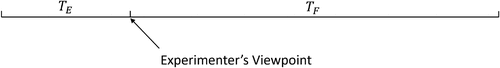
The experimenter is interested in understanding the effects of a long-term treatment, yet they can only run the experiment for a shorter duration. We explain the horizon as follows. Let there be a discrete, finite time horizon consisting of time periods in chronological order. Out of these T time periods, the first time periods are referred to as the experimental periods, and the last time periods are referred to as the future periods. After conducting the experiment until the end of the experimental periods , the experimenter has access to data collected from periods 1 to , and is interested in some causal effects that will not be directly observed until the end of period T. In our running example, the experimenter could run the experiment for a few weeks, and then use the experimental data to estimate what would happen if the intervention continues to last for additional weeks. See Figure 1 for an illustration.
We consider two versions of treatments although our approach can easily extend to multiple treatments. One version is the control condition (or, simply, “control”), which represents the status quo of the product; the other version is the active treatment (or, simply, “treatment”), which represents the product with the new feature. Let be the random treatment assignment that subject receives in time period . takes values from , where 0 stands for control and 1 stands for treatment. For each subject, we use to stand for the treatment assignments that subject receives during periods 1 to t. Following convention, we use to stand for a random treatment assignment and to stand for one realization. When the subscript i is clear from the context, we sometimes drop it for brevity, and write instead.
We conduct a randomized experiment wherein once a subject is assigned into either the treatment or control group, it stays in that group during the entire horizon. If subject i is assigned into the treatment group, then ; if subject i is assigned into the control group, then , where we use and to stand for a length-t vector of ones and zeros, respectively. As we stand at the end of period , we have only conducted the experiment during the first experimental periods, and not yet in the last future periods.
We do not consider other types of treatment patterns that change the treatment assignment in the middle of the horizon, such as a step-wedge design (i.e., a staggered adoption pattern; Brown and Lilford 2006, Hussey and Hughes 2007, Hemming et al. 2015, Li et al. 2018, Xiong et al. 2019) or a switchback design (Cochran et al. 1941, Glynn et al. 2020, Hu and Wager 2022, Bojinov et al. 2023, Xiong et al. 2023). This implies that, for simplicity, we could just use a single binary variable to indicate if a subject is assigned to the treatment or control group. But for clarity, we would rather carry the treatment assignment vector. Although the treatment assignments remain the same over time, the treatment probabilities across different subjects can be different. Our framework allows treatment assignments to be dependent on (i.e., stratified randomization), although we have only conducted complete randomization in our empirical execution.
During the experimental periods, the experimenter observes several quantities of interest. For each subject and at each time period , the experimenter observes a primary outcome that takes values from and D intermediate outcomes that take values from . In our running example, the primary outcome could be the click-through rate and the intermediate outcomes could include a number of user activity metrics such as log-in frequency, average usage duration, number of total searches, and the numbers of searches in each category.
Following the potential outcomes framework (Neyman 1923) and under the Stable Unit Treatment Value Assumption (Rubin 1974, Holland 1986, Imbens and Rubin 2015), each subject at each time period has a set of potential outcomes and . Each observed outcome, either the primary outcome or the intermediate outcome, is related to its respective potential outcomes as follows,
During the future periods , we could also define the same quantities as above, although the observed outcomes have not been observed by the experimenter. See Table 1 for an illustration of our problem setup and summary of notations.
|

Table 1. Illustration of Our Problem Setup and Summary of Notations
| Groups | Experimental periods | Future periods |
|---|---|---|
| Treatment group | , observe | Missing |
| Control group | , observe | Missing |
Note. The treatment assignments , primary outcomes , and surrogate outcomes are all missing from the future periods, as our viewpoint is at the end of the experimental periods.
In addition, let be some pretreatment intermediate outcomes at time 0, which may reflect subject-level heterogeneity before the experiment. For notational convenience, we collect and to be all the potential outcomes. Further, we introduce a short-hand notation to emphasize the most recent treatment assignments. For any and any , if , then we write . Note that this is only a short-hand notation, and does not impose any assumptions.
In this paper, we postulate a superpopulation that each subject is sampled from with replacement, so that each subject is identically and independently distributed. For each , let be the joint probability distribution that is sampled from. There are two sources of randomness in our experiment: one comes from the randomized experiment, that is, the treatment assignments are random; the other comes from the sampling from a superpopulation, that is, the pretreatment variables and all the potential outcomes are random.
The experimenter is interested in understanding the average effect of long-term treatments on the primary outcome,
Such causal effects often emerge when experimenters aim to permanently launch a new product. In our running example, this relates to click-through rates over weeks or months.
2.2. Conventional Wisdom and New Challenges
In this paper, the duration of treatments spans the entire horizon, which we refer to as long-term treatments. To estimate the effects of long-term treatments, the ideal approach is to conduct experiments for an extended duration of time in the future periods and directly estimate from such an ideal experiment. However, as discussed in Section 1, the experimenter is often unable to assign treatments for a long-term duration, and there is no observation from the future periods at the moment of estimation. The fundamental challenges associated with this problem are two-fold:
(Missing treatments) At the moment of estimation, the experimenter has not conducted any treatment in the future periods.
(Missing observations) At the moment of estimation, the experimenter has not observed any outcome in the future periods.
The presence of the above two challenges requires a new method that explicitly considers the longitudinal nature of the treatments, where the existing surrogate approach (Prentice 1989, Weir and Walley 2006, Joffe and Greene 2009, Yang et al. 2023, Athey et al. 2025) does not directly apply. For example, Athey et al. (2025) and Yang et al. (2023) examine the treatment effects where the duration of treatments is relatively short compared with the length of future periods and the treatments never occurred during the future periods. We thus refer to the effect they studied as the long-term effects of short-term treatments; in other words, they focus on estimating the long-term “carryover effects,” that is,
Therefore, the existing surrogate approach addresses the second challenge only and establishes a surrogate predictor using the historical data, which are used to extrapolate from the short-term observations. Unless the treatments in the future periods have no direct effects, that is, , the existing surrogate approach will lead to biased estimation of , the average effect of long-term treatments.
To address the above two challenges, we propose a framework to extend the existing surrogate approaches to the longitudinal setting discussed above. Below, we introduce a few identification assumptions that we make in the longitudinal surrogate framework.
2.3. Identification Assumptions
Below, we first introduce the longitudinal surrogate model and the two required identification assumptions. These two identification assumptions are what we refer to as the first level of assumptions. Because the longitudinal surrogate model may suffer from the potentially limited sample size (see Section 3.1 for details), we introduce an additional assumption to the first level of assumptions, leading to the linear surrogate model.1
2.3.1. Longitudinal Surrogate Model.
We start with the basic assumptions that lay out the foundations of estimating the causal effect. There are two such basic assumptions.
(
Moreover, we refer to the intermediate outcomes at the time periods as surrogate outcomes, or, simply, surrogates.
Assumption 1 is the longitudinal extension of the surrogacy assumption in the literature (Prentice 1989, Weir and Walley 2006, Joffe and Greene 2009, Yang et al. 2023, Athey et al. 2025). Intuitively, Assumption 1 implies that the surrogate outcomes at a middle period fully saturate the causal link between the treatment assignment at an earlier period and the primary and intermediate outcomes at a later period. In other words, there is no effect of the treatment assignment at an earlier period on the primary and intermediate outcomes at a later period that does not pass through the surrogate outcomes at the middle period. See Figure 2 for an illustration using the directed acyclic graph representation (Pearl 1995). We discuss practical guidelines for choosing surrogates in Online Appendix Section D.
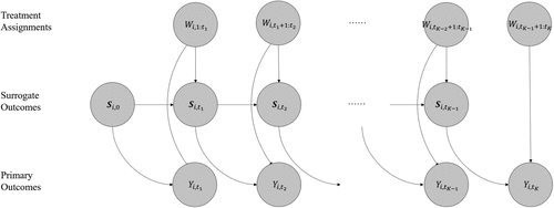
Notes. In this illustration, each solid line represents a causal path. Each treatment assignment at an earlier period impacts the surrogate outcomes and the primary outcome at a later period; each surrogate outcome and the primary outcome at an earlier period impact the primary outcome at a later period. Each treatment assignment at an earlier period does not directly impact the primary and surrogate outcomes at a later period without going through the surrogate outcomes and the primary outcome at the middle period. For simplicity, pretreatment variables are not explicitly included in this figure. However, the subscript i in the surrogate and primary outcomes implicitly suggests that we could incorporate pretreatment variables.
There are two direct implications of Assumption 1. The first implication is that, if Assumption 1 holds for some , it also holds for any subset of ; that is, for any , Assumption 1 also holds for . The second implication is that, for any , any , and any ,
This is because, if and are not independent, then and will not be independent, violating Assumption 1.
In the longitudinal surrogate model, the surrogate outcomes serve as critical links in the causal diagram in two ways. First, conditional on the surrogate outcomes, we extrapolate to the primary outcomes in the future periods using what we refer to as the longitudinal surrogate index, which we define in Definition 1. Second, conditional on the surrogate outcomes at an earlier period, we build our understanding of the future surrogate outcomes using what we refer to as the pivot index, which we define in Definition 2.
(
Intuitively, the longitudinal surrogate index serves as a prediction of future primary outcomes using the current intermediate outcomes, the pretreatment variables, and the treatment assignments. This index has a time-dependent subscript, which reflects the longitudinal nature of our setup, and is different from the surrogate index as originally defined in Athey et al. (2025).
In addition to the longitudinal surrogate index, we introduce the pivot index as defined below.2
(
The pivot indices (or the conditional surrogate outcomes, depending on which identification strategy to use) are the key idea behind our longitudinal surrogate framework. “” indicates following the same distributions. Intuitively, they bridge the surrogates at the earlier periods and the surrogates at the later periods. The use of pivot indices is necessary in our model because the experimental duration is short, and what we learn from the experimental data needs the pivot indices (or the conditional surrogate outcomes) to iterate and extrapolate to the future periods. Note that the definition of pivot indices replaces the primary outcomes as defined in Definition 1 by the surrogate outcomes.
(
Intuitively, Assumption 2 implies that the relationship between the primary and intermediate outcomes at a later period and the intermediate outcomes at an earlier period is the same at other time periods. So, we could use data collected from the experimental periods to learn the relationship and apply it to future periods. Note that Assumption 2 does not necessarily assume the primary outcomes or the surrogate outcomes are time-homogeneous; instead, Assumption 2 assumes the functions of the surrogate index and the pivot indices to be time-homogeneous.
Assumptions 1 and 2 are the most basic level of assumptions. Under Assumptions 1 and 2, and using the succinct notations from Definitions 1 and 2, we present the first identification result as follows.
We first introduce a special case to illustrate the key idea behind our main theorem.
Consider the special case when . Under Assumptions 1 and 2, where Assumption 1 holds for , the average effect of long-term treatments on the primary outcome is equal to the following expression:
Lemma 1 consists of two components: the surrogate index component that predicts the primary outcomes using the pivots and a conditional surrogate outcomes component that reweighs the distributions of the random surrogate outcomes using the pretreatment surrogate outcomes. Lemma 1 illustrates how the surrogate outcomes at as the outputs of the inner loop reweighting are used as the input of the outer loop surrogate index. The surrogate outcomes at effectively serve as the link between the two components.
In the more general setting when , we need to have more surrogate outcomes to serve as the links. We split the horizon of T periods into several intervals, each length of which is no larger than the length of the experimental periods. Mathematically, denote . The above condition suggests that . We write and as the end and start of all periods. Then, we apply the same method as in Lemma 1 on each interval and update the surrogate outcomes iteratively. We formalize the above intuition as follows.
(
Theorem 1 consists of a sequence of iterative components. There is one surrogate index component that predicts the primary outcomes during the last interval, using the conditional surrogate outcomes reweighted from the second last interval. There is a sequence of conditional surrogate outcomes that reweighs the distributions using the conditional surrogate outcomes reweighted from the previous interval. Both components (i.e., the surrogate index and the conditional surrogate outcomes) can be estimated from the data during the experimental periods.
2.3.2. Linear Surrogate Model.
Although general, the first identification strategy as suggested by Lemma 1 and Theorem 1 suffers from a major challenge resulting from the random nature of conditional surrogate outcomes and potentially limited sample sizes. We will revisit this challenge in greater detail in Section 3.1. To address this, we introduce an additional assumption to the two basic assumptions. This set of three assumptions is the second level of assumptions.
(
The surrogate index function is linear with respect to the surrogates; that is, there exists , , such that
(2)The pivot index function is linear with respect to the surrogates; that is, there exists , , such that for each ,
(3)where stands for the d-th component of , the pivot index.
Assumption 3 specifies a linear functional form to the surrogate index and the pivot index. It is worth mentioning that Assumption 3 assumes both the surrogate index and the pivot index to be linear with respect to the surrogates, but not necessarily with respect to the pretreatment variables. Under this additional Assumption 3, we simplify Theorem 1 and introduce the second identification result as follows.
(
Theorem 2 involves both the surrogate index and the pivot index. The input of an outer iteration is the output of an inner iteration, which, under the linearity assumption, is simply the pivot index in the inner iteration. With this linear model, the identification strategy as suggested by Theorem 2 properly mitigates the issues of large sample sizes as required by the longitudinal surrogate model, and thus estimates the future treatment effects with reasonable sample sizes.
3. Estimation and Inference
In this section, we discuss the estimation strategies, inference strategies, and model validation strategies for the models discussed above. We focus on conventional randomized experiments where subjects are randomly assigned into the treatment or the control groups under (covariate-independent) complete randomization. Let and be the number of users in the treatment and the control group, respectively, which are fixed quantities under complete randomization. Our approach readily applies to more general randomization schemes, which we omit in this paper.
3.1. Estimation Strategies
Recall that in Section 2.3 we introduce two levels of identification assumptions. Below, we introduce two estimation strategies, each requiring one level of assumptions discussed in Section 2.3.
3.1.1. Estimators for the Longitudinal Surrogate Model.
Given estimators of the surrogate index and estimators of the conditional surrogate outcomes, we follow Theorem 1 and obtain the following plug-in estimator:
We explain how to estimate the surrogate index functions in (4). For any , , , one naive estimator of the surrogate index under consecutive controls is given by
Under complete randomization, such an estimator is unbiased for the surrogate index function. Similarly, for any , , , one naive estimator of the surrogate index under consecutive treatments is given by
Under complete randomization, such an estimator is unbiased for the surrogate index function. Yet given the oftentimes multidimensional nature of and , and the limited number of treatment subjects in the experimental periods, the above two estimators are not always well-behaved. For each combination of and , we need a sufficiently large number of samples in the experimental periods to have reasonably accurate estimation, which is often challenging in practice.
3.1.2. Estimators for the Linear Surrogate Model.
Because of the limitations of the longitudinal surrogate model, we introduce the linear surrogate model, which requires the additional Assumption 3. Given the surrogate and pivot index estimators, we follow Theorem 2 and obtain the following plug-in estimator:
Note that because is directly observable, we can use the observed to replace in the first (inner) plug-in. We use the following plug-in estimator in empirical estimation:
We explain how to estimate the surrogate and pivot index functions in (6). We first consider a proper discretization of the pretreatment variables . Then, for each and under homoscedasticity, a naive estimator of the coefficients of the surrogate index function is given by
The above two least squares estimators find the coefficients for any . This is suitable when the pretreatment variables are low-dimensional and discrete. Given the multidimensional nature of , and especially when is continuous, the least squares estimators are not always well-behaved. To address the above concern, we could include the pretreatment variables in the least square term instead of conditioning on them. Instead of estimating and , we pool the data and run the following linear regression to estimate and , as well as and :
The second part in (6) can be estimated similarly. The above expressions find the best linear unbiased estimator for the coefficients of the pretreatment variables. They mitigate the issue of requiring a large sample size in the longitudinal surrogate model.
3.2. Inference and Testing
Our estimator leverages an additional layer of randomness from the random treatment assignments. Here, we propose Fisher’s exact test to draw inference from the collected data. We consider the following sharp null hypothesis of no treatment effect at any time period for any subject:
We can conduct exact tests by leveraging the completely randomized experiment to simulate new treatment assignments; see Algorithm 1 in the Online Appendix. To obtain a confidence interval, we propose inverting a sequence of exact hypothesis tests to identify the region outside of which (7) is violated at the prespecified nominal level (Imbens and Rubin 2015, chapter 5). Alternatively, one could also use bootstrap to obtain a confidence interval. The source of randomness comes from our random treatment assignments; see Algorithm 2 in the Online Appendix. In later empirical sections, we mainly report the results using the bootstrap method.
Our work is also related to forecasting methods in the time series analysis and the macroeconometrics literature, such as autoregressive models, the VAR model, and Autoregressive Integrated Moving Average (ARIMA) (Stock and Watson 2001, 2020; Andersen et al. 2003; Fuller 2009; Hamilton 2020). The macroeconometrics literature has also provided ways to construct confidence intervals by leveraging the randomness of the joint probability distribution that is sampled from. Such confidence intervals are generally recognized to have more power than Fisher’s exact test, which relies on the randomness of the random treatment assignments. For simplicity, we adopted the simpler approach of Fisher’s exact test and the bootstrap method.
3.3. Validation of Assumptions
As the longitudinal surrogacy (assumption Assumption 1) and the comparability (assumption Assumption 2) play a critical role in determining the validity of our method in practice, we explore approaches to validate whether these assumptions are satisfied in this section.3
3.3.1. Validation of Assumption 1.
Similar to the tests on the validity of instrumental variables, Assumption 1 cannot be directly tested. Instead, we propose conducting a sensitivity analysis to determine how sensitive the treatment effect estimation is when Assumption 1 is violated. Our approach is inspired by the literature on sensitivity analysis of instrumental variables (Baiocchi et al. 2014). Arguably, the most common violation of Assumption 1 occurs when there are omitted surrogates. Figure G.12 in the Online Appendix illustrates such a scenario: Assumption 1 is violated because the treatment assignment during the experimental periods affects the primary outcome through both variables and . Here, only are considered as the surrogate variables, whereas represent the omitted surrogates that remain unidentified or uncollected.
First, a straightforward approach for sensitivity analysis on Assumption 1 is to assess the fluctuation in estimation given that only a subset of surrogate outcomes are applied as surrogates. This analysis reveals how the estimation is impacted by the exclusion of certain already-collected surrogates. We demonstrate that as more surrogates are removed, the estimation performance deteriorates, aligning with our intuition. Overall, our estimation approach is relatively robust across different subsets of surrogates. Detailed analysis of this approach is provided in Online Appendix G.1.
Second, we design an approach to test the sensitivity of omitted surrogates, focusing on assessing the model’s sensitivity to surrogates that were never observed. This approach can be particularly valuable in real-world experiments where some of the surrogates can be potentially unobservable and missing from our estimation. Our method can be seen as an adaptation of the sensitivity analysis for assessing the Exclusion Restriction assumption for instrumental variables (Baiocchi et al. 2014).
Suppose, for any , , and , the treatment assignment affects the primary outcome not only through the identified surrogates but also via a missing variable . We create this variable following a normal distribution with mean zero, and variance equal to the average variance of the Y during the experimental periods. We manually introduce an additional causal path between the treatment assignment and the primary outcome through variable :
3.3.2. Validation of Assumption 2.
We begin by introducing a straightforward test directly for Assumption 2 (the comparability assumption). Moreover, we discuss that even when Assumption 2 does not hold, we can still apply our longitudinal surrogate framework, by leveraging a relaxation of Assumption 2, which we refer to as the Parallel Trends assumption (Assumption 2′). We also provide a test for this parallel trends assumption.
3.3.2.1. Direct Test for Assumption 2.
The objective of this test is to identify matched observations across two distinct time periods, t and , based on exact matching criteria involving the surrogates , the treatment assignments , and the pretreatment variables . More specifically, we begin by specifying the two time periods of interest, t and , and the lag parameter . For each unit i at time t, we collect the following information: , and . Next, we search for any unit at time that satisfies the following conditions:
All pairs of observations that meet the above conditions are included in the analysis pool, which results in two groups of observations from each of the two time periods t and , with the corresponding outcomes . If no observations meet the requirement at time t, the test for that specific condition is excluded from further analysis. For each possible combination of , we perform statistical tests to examine the difference between and and report p-values.
3.3.2.2. Parallel Trends Test.
To make our longitudinal surrogate framework more useful to practitioners, we relax Assumption 2 to Assumption 2′, which we call the Parallel Trends assumption. When combined with the linearity assumption and under certain conditions, this new assumption still guarantees that Theorem 2 holds. The detailed theory of Assumption 2′ is presented in Online Appendix F. Assumption 2′ can be more robust to real-world settings.
Below, we introduce a statistical test to evaluate whether the parallel trends assumption holds by focusing on two distinct time periods, denoted as t and , along with a specified positive integer . The first step is a matching procedure. For each unit i in the treatment group characterized by the preperiod surrogates and pretreatment covariates at time t, where the treatment assignment satisfies , we identify an exact match in the time period . The matching criteria require that the matched unit satisfies
Upon locating an exact match, one observation from period is randomly selected to form a matched pair within the treatment group. Observations without an exact match are excluded from the evaluation. This matching process is similarly applied to the control group, where the treatment assignment condition is , resulting in matched pairs within the control group.
The second step is a regression analysis. This exact matching ensures that the paired observations in both the treatment and control groups are conditioned on identical distributions of preperiod surrogates and pretreatment covariates. The regression model is specified as follows for the matched pairs only:
We estimate the parameters of this regression model and conduct a t-test for the null hypothesis Failure to reject suggests that the parallel trends assumption may not be violated. Note that a comprehensive discussion on the validation of the comparability assumption and parallel trends assumption, including theorem, related proof, and the statistical testing results derived from empirical experiments, is provided in Online Appendix F.
4. Empirical Validation
We collaborated with WeChat and analyzed two real-world long-term experiments on WeChat Search to validate the effectiveness of our proposed approach.4 WeChat Search serves as a function within WeChat, enabling users to search for information both internally and externally to the WeChat platform.5 These experiments offer valuable data, enabling us to observe the ground truth of treatment effects in the future periods and compare them with our estimates made at the end of the experimental period.6 Sections 4.1 and 4.2 offer detailed descriptions of the experiment background and our empirical strategy and results.
After analyzing the experimental results, we further validate the effectiveness of our approach using multiple synthetic experiments, detailed in Section 4.3. These synthetic experiments discuss scenarios not necessarily represented in the two real-world experiments, offering a thorough examination of our proposed method. In Section 4.4, we provide additional robustness analyses of our real-world experiments.
4.1. Experiment 1: Mini-programs in Search History
4.1.1. Experiment Background.
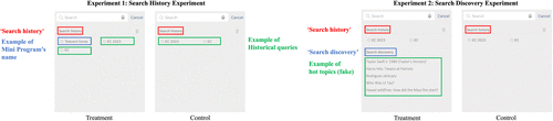
Similar to many other social media platforms, WeChat provides a search box that allows users to search for a variety of embedded WeChat features, such as chat history, news articles, and mini-programs (embedded third-party apps). In Experiment 1, practitioners aimed to test whether displaying recently searched mini-programs as part of the search query history in the search box would affect user activity on WeChat Search.
As presented in Figure 3, the “search history” panel provides a shortcut for users to quickly access the search results of keywords they previously searched. In the treatment condition, the experiment extended the functionality of the “search history” panel by providing additional shortcuts to access mini-programs that users had recently used. The control condition did not show this new function and remained as the status quo. The experimenters hypothesized that with this new feature, users would be more likely to visit their frequently used mini-programs through the shortcuts provided by WeChat Search, rather than swiping down on WeChat and scrolling to find the target mini-programs. The business objective of this treatment was to encourage users to engage more with WeChat Search, thereby increasing its user engagement. Figure 3 illustrates the user interfaces for both the treatment and control groups.
In the experiment, about 1.3 million users were randomly assigned to treatment or control groups. The treatment group consists of 667,206 users, whereas the control group consists of 665,830 users. The primary outcome of interest is weekly search_uv, the average number of days that a user has searched in a week.7 During this seven-week experiment, the results showed a positive treatment effect with a sharp increasing trend in the short term (the first two weeks), setting high initial expectations for the new feature’s potential. However, the positive treatment effect becomes stable, albeit slightly diminished, in the long term (see the trends for the ground truth in Figure 4(a)). As a result, the treatment was launched to all users after the experiment.
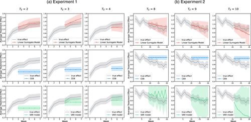
Notes. Dashed curves represent the true average treatment effect on search_uv from week 1 to week 7 for Experiment 1 (from week 1 to week 20 for Experiment 2). Solid curves in the first row represent the estimated effects with the linear surrogate model. Solid curves in the second row are the Constant Extrapolation Baseline that uses the short-term effect to extrapolate. Solid curves in the third row are the estimated effects with the VAR model. Shadows indicate 95% confidence intervals. The three panels represent the scenarios when we use the first weeks as the experimental period and the last weeks as the future period. For in VAR, a constant extrapolation is used because of the limited length of the time series.
For randomization checks, we performed two tests. First, we conducted the sample ratio mismatch (SRM) test (Fabijan et al. 2019), which uses chi-squared tests to examine whether the sample sizes of the two groups are not significantly different, as 50% of the number of experiment participants were assigned to each group. The experiment passed the chi-squared test, indicating no sample ratio mismatch problem. Second, we observed that there were no significant differences in the pretreatment variables between the two groups before the experiment. We performed t-tests for mean comparisons, where all the p-values are larger than 0.1, suggesting the insignificant differences and the validity of our randomization process. See details in Online Appendix E.2.
4.1.2. Empirical Strategy.
In our analysis, we divided the seven-week experimental period into two phases: the experimental periods 1 to and the future periods to T. During the experimental periods, we collected data and observed the effects of the treatment. After the experimental periods end, our goal is to predict the treatment effects for each week in the future periods, starting from week and continuing through the last period. While making these predictions, we do not use data from the future periods, as they have not been observed yet at time . We use our model to estimate the treatment effects during the future periods. Finally, we compare these estimated effects with the actual treatment effects observed during the future period. These observed effects in the long-term experiment serve as the “ground truth” to evaluate the accuracy of our approach.
We consider variables that capture various aspects of user behavior during the search process as our surrogates. Detailed descriptions of all surrogate and primary outcomes are provided in Table E.1 in the Online Appendix. These surrogates not only are responsive to the treatments but also reflect the diverse aspects of user behavior that lead to variations in primary outcomes over time (Deng et al. 2013, Duan et al. 2021). Note that we include past primary outcomes as a subset of the surrogate variables, as they are shown to be useful in modeling the future primary outcomes (Deng et al. 2013). This is a little different from the causal diagram shown in Figure 2, yet this still satisfies Assumption 1. To see this, consider the following simplest example with only two periods and for any . Let the surrogates consist of two parts , where and are primary outcomes and are the other surrogate outcomes. We still have
Note that we not only use surrogates from the immediate preceding time period but also incorporate surrogates including primary outcomes from earlier periods— up to —into our model. For example, search_uv in period can be seen as the “search_uv two weeks ago,” which is then used as a surrogate in period t. Therefore, to establish the models, we use the surrogates (including the primary outcomes) from week 1 to week in total to be our training features, and the surrogates and primary outcome of the week serve as the training outcomes. As we have five surrogate variables, our prediction model has training features.8 By employing this approach, we effectively broaden the surrogate space, thereby enhancing the precision of our predictions.
After establishing the models for the primary outcome and surrogates, we iteratively use each model to estimate surrogate and primary outcome values for each week during the future period, that is, . Note that the prediction model is not supposed to have access to the actual values of any surrogates or primary outcomes post-. Consequently, the input features for each model are based on both the observed surrogate and primary outcome values during the experimental periods and their predicted values post-. For example, we employ observed surrogates from weeks 2 to to project those in , and then we utilize the surrogates observed from weeks 3 to as well as the surrogates previously predicted for time to estimate those in (and so on). With this iteration, we are able to predict both primary outcomes and surrogates until time T.
We focus on presenting the results from our main model, the linear surrogate model.9 We construct confidence intervals using the bootstrapping technique (Efron 1987, Efron and Tibshirani 1994). We use a bootstrapping approach to estimate the confidence intervals for the long-term treatment effects. We resample 50% of the users with replacement to create each replica, selecting half of the original sample to form a new subsample.10 For each replica, we build a separate prediction model using only this subsample. Based on this model, we then estimate the long-term treatment effects for each replica. This process is repeated 100 times to determine a 95% confidence interval for the true treatment effect. This method allows us to account for variability from both the random assignment of subjects and the model itself.
4.1.3. Baselines.
We employ two different baselines with confidence intervals using the same bootstrap technique described above.
CEB: We use the average treatment effects observed during the first weeks of the experiment to predict the treatment effects for the future period. Although obviously this approach cannot capture any increasing or decreasing trends in the treatment effects, this serves as a common industry practice.
VAR model: We employ a VAR model with lag order on the initial weeks of the multivariate time series, using the average values of four surrogates and one primary outcome variable as input candidates. This allows the VAR model to forecast future outcomes based on past values of all included variables, though VAR is traditionally used for forecasting rather than causal inference (Stock and Watson 2001).11
4.1.4. Results.
We present the estimates of the linear surrogate model, the baselines, and true effects in Figure 4(a). We vary the value of from two to four to ensure that is meaningfully short compared with the entire duration, constituting around half or less of the entire horizon. We observe that the CEB consistently underestimates the effects of long-term treatments. The vector autoregressive models perform slightly better than CEB, especially when is larger. However, these baseline models cannot predict the long-term increasing trend of the treatment effect.
By contrast, our estimation, indicated by red curves in Figure 4, can successfully capture an increasing trend in the treatment effect regardless of the choice of . For instance, our estimation successfully predicts both a long-term increasing trend at and a stable trend at , which other baseline models fail to do. In practice, successfully predicting the trend of treatment effects over time is critical for making product decisions. In addition, using the first two weeks only, our estimation of the effect of long-term treatment in week 7 is 1.347, which is less biased compared with the true effect (1.278) compared with baselines.
Further, we compare the bias and MSE between our model and the baselines. Specifically, we present their averages over all weeks during future periods and present the results in Table 2. Overall, considering the three choices of , our model consistently outperforms the baseline model in terms of bias, and outperforms the baseline model in terms of MSE in the majority of cases. These results further underscore the effectiveness of our approach.12
|
Table 2. Comparison Result Between Different Methods in Terms of Bias and MSE for Experiment 1
| Method | Bias | MSE | ||||
|---|---|---|---|---|---|---|
| Linear surrogate model | 0.087 | 0.199 | 0.165 | 0.327 | 0.324 | 0.314 |
| CEB | 0.479 | 0.401 | 0.393 | 0.342 | 0.263 | 0.243 |
| VAR model | 0.479 | 0.210 | 0.174 | 0.342 | 0.328 | 0.435 |
As increases, an estimation model is generally expected to have higher bias and MSE, as predictions are made further into the future and are less anchored by current observations. However, temporal fluctuations—such as seasonal effects, holidays, and rare events—can introduce additional complexity that disrupts this trend. Such events can make certain short- or medium-term periods more challenging to predict accurately than other periods further in the future. As a result, although a general increase in bias and MSE with forecast horizon length may hold, this trend is not strictly monotonic and can vary based on the occurrence of these less predictable events.
We also examine whether the surrogacy and comparability assumptions hold for the experiment using the methods proposed in Section 3.3. First, we conduct a sensitivity analysis for the surrogacy assumptions, presenting the results in Online Appendix G.1 and Online Appendix G.2, to demonstrate the robustness of our estimation to the potential of omitted surrogates. Moreover, we perform both the tests for comparability and parallel trends assumptions. Detailed results are presented in Online Appendix F.1 and Online Appendix F.5.
4.2. Experiment 2: Search Discovery
4.2.1. Experiment Background.
Similar to Experiment 1, Experiment 2 also involves a change in WeChat Search. Instead of adding shortcuts to mini-programs in the “search history,” practitioners aimed to test whether displaying hot topics as part of the search discovery in the search box would affect user activity on WeChat Search. The experimenters hypothesized that with this new feature, users would be more likely to read and engage with these new shortcuts to trendy topics. The business objective of this treatment was to encourage users to engage more with WeChat Search, thereby increasing its user engagement. Figure 3 illustrates the user interfaces for both the treatment and control groups. In the treatment condition, the users were offered this new feature, whereas in the control condition the users were not. However, the long-term effect of this treatment remains uncertain and critical because including this new panel of hot topics might also crowd out users’ intention to search. Different from Experiment 1, where the new feature mainly assists in searching for the mini-programs based on individuals’ search history, the new feature for Experiment 2 is to provide shortcuts that help users to explore hot topics, which might affect their initial search intention. Thus, WeChat launched this experiment for a total of 20 weeks.
This 20-week experiment involves 3.6 million WeChat users. Among them, 1,807,335 users were randomly assigned to the treatment group, whereas 1,803,675 users were randomly assigned to the control group. Again, the primary outcome of interest is search_uv. Because both experiments focus on WeChat Search and share the same primary outcome, the same set of surrogates described in Table E.1 in the Online Appendix is used for Experiment 2. In this experiment, the goal is to predict the treatment effects over a long period until period T (the 20th week) using the data available at the end of period .
To examine the validity of randomization, we also performed the SRM test and mean comparisons on the pretreatment variables between the treatment and control groups, similar to Experiment 1. The results confirm the validity of our randomization process, showing that there is no statistically significant difference in the sample sizes and no statistically significant differences in the pretreatment variables between the two groups. More details are discussed in Section E.2 of the Online Appendix. In addition, we present the summary statistics in Table E.2 of the Online Appendix.
The average treatment effect shows continuous fluctuations without an apparent downward trend signal in the first seven weeks, whereas these are followed by a continuous decline after eight weeks of treatment over time. It is suspected that there is a long-lasting novelty effect for this treatment, and the effect is likely to decay over time. As a result, this new product change (treatment) was not eventually adopted or launched to all users. Nevertheless, the valuable insights gained from this experiment have inspired the development of other significant product strategies.
4.2.2. Empirical Strategy, Baselines, and Results.
Both experiments conducted on WeChat Search have the same primary outcomes and surrogates, so we use the same empirical strategy as in Experiment 1. The potential consistency of surrogates among different experiments can enable easy scalability of our approach in practice. Because this experiment is longer (20 weeks), we employ the linear surrogate model and showcase results for () in the main text, while presenting results with different choices of () in Online Appendix E.3. Additionally, we use the same baselines for validation in Experiment 2 as those in Experiment 1 for consistency.
The estimation results are presented in Figure 4(b). We observe that our approach effectively captures the decreasing trend of the average treatment effect in the long run. By contrast, the CEB model consistently overestimates the treatment effects during the future period , as it fails to capture the decreasing trend of the treatment effect. The VAR model exhibits fluctuating estimates over time and unstable prediction trends across different experimental periods , because of the volatility of the primary outcome (Y), search_uv, over time in both the treatment and control groups. The VAR model appears to be unable to handle this scenario well.
Table 3 reports the average bias and MSE over the future periods for each . Consistent with the results from Experiment 1, our method outperforms both baseline models (CEB and VAR) in terms of bias across all values of . As the forecast horizon extends beyond the experimental period, our model tends to exhibit increased estimation variance for more distant future periods. This phenomenon occurs because errors in near-term predictions can propagate and amplify when used as inputs for subsequent, longer-term forecasts. A similar issue arises with the VAR baseline model, which also relies on near-future periods’ information for extended predictions. Despite both our method and the VAR model exhibiting higher variance compared with the trivial constant extrapolation, we consider this an acceptable bias-variance tradeoff. Similar to Experiment 1, we conduct analyses proposed in Section 3.3 to examine surrogacy and comparability assumptions. We demonstrate our estimation’s robustness to both assumptions and present the results in Online Appendices G.1, G.2, F.1, and F.5.
|
Table 3. Comparison Result Between Different Methods in Terms of Bias and MSE for Experiment 2
| Method | Bias | MSE | ||||
|---|---|---|---|---|---|---|
| Linear surrogate model | 0.098 | 0.048 | 0.158 | 0.233 | 0.136 | 0.201 |
| CEB | 0.274 | 0.272 | 0.258 | 0.106 | 0.103 | 0.096 |
| VAR model | 0.240 | 0.054 | 0.565 | 0.520 | 0.645 | 2.552 |
4.3. Simulations Using Synthetic Data
In addition, to encompass scenarios not necessarily represented in the real-world experiments, we undertake synthetic experiments for a more thorough evaluation of our approach.
4.3.1. Stabilized Treatment Effect.
In our synthetic experiments, the first scenario we investigate is when the effects of long-term treatments plateau or stabilize over time. To illustrate this, we set up the following synthetic experiment: The simulation presupposes four surrogates, , for each time period t and unit i. For each dimension d, each of its corresponding surrogates draws from a normal distribution, . Surrogates in different dimensions are independent from each other. In this synthetic experiment, subjects assigned to the control group experience no deviation from the status quo; as a result, the surrogates’ distribution remains unchanged. In contrast, for those in the treatment group, there is a time-dependent decay in the four surrogates, governed by decay factors , respectively (e.g., ). In order to comply with both the surrogacy and linearity assumptions, the primary outcome, , is designed as a linear combination of these four surrogates.
In the first synthetic experiment, we set the parameter and , and the primary outcome Y in period t is formulated as . In this setup, the effect of long-term treatments on initially increases and then stabilizes, showcasing a characteristic “leveling-off” pattern. Using experimental data spanning periods, we compare our approach’s estimates with the true future effects. The first row of Figure H.18 in the Online Appendix demonstrates a precise estimation of the effects of long-term treatments.
The second simulation shares the settings with the first one except for the parameter and , and the primary outcome being formulated as .13 This configuration leads to the effect of the long-term treatment on Y initially declining and then stabilizing, exemplifying another typical “leveling-off” trend. The first row of Figure H.19 in the Online Appendix presents the estimation results, demonstrating that our approach can accurately capture the future treatment effects.
In both synthetic experiments, our estimates closely align with the true effects of long-term treatment, demonstrating our approach’s capability to account for scenarios where treatment effects stabilize over time. Figures H.18 and H.19 in the Online Appendix showcase the graphical comparison between our approach and all the other baseline models, including the CEB model and the VAR model in two synthetic experiments. Moreover, numerical comparison between our approach and multiple baselines in terms of bias and MSE is provided in Tables H.10 and H.11 in the Online Appendix. Our approach surpasses all of the baseline models in both synthetic experiments regarding bias and MSE. Collectively, these analyses further show the validity and generalization of our approach to various empirical settings.
Further, we performed a sensitivity analysis for the surrogacy (assumption Assumption 1) on both of the two synthetic experiments to demonstrate the relationship between the degree of violation of Assumption 1 and estimation accuracy. The results in Online Appendix G.1 show that performance worsens with more severe violations of Assumption 1, but a longer observational experimental period can mitigate this deterioration to some extent.
4.3.2. Additional Synthetic Experiments.
To complement our real-world experiments, we conduct additional synthetic experiments that challenge certain assumptions or alter the behavior of long-term treatment effects. We explore two scenarios.
4.3.2.1. Violation of Comparability.
In this experiment, we create synthetic contexts where the comparability assumption may not hold and test whether our framework can detect these violations, as well as observe how its performance changes accordingly. We simulate scenarios with varying degrees of comparability assumption violations. In this simulation, the primary outcome for users in the treatment group is defined as . When and i is in the treatment group, we vary over the values [1, 1.5, 2, 2.5, 3] to control the extent of the comparability violation. For all other time periods for the treatment group and for all time periods in the control group (including ), we set . We demonstrate that both the comparability and parallel trends assumption tests we proposed can effectively detect this violation. Moreover, as the degree of violation increases (i.e., as becomes larger), estimation bias increases accordingly. Please refer to Online Appendix H.2 for more details.
4.3.2.2. Nonlinear Outcome Function.
Although our main results rely on the linearity assumption in the linear surrogate model, we also create synthetic contexts where this assumption may not hold and test how our method’s performance may be affected. We evaluate our method under a nonlinear outcome function by introducing two surrogates and . The primary outcome is , where adjusts the degree of nonlinearity. Note that to create the treatment effect, we allow the surrogates in the treatment group to decay over t, whereas the surrogates for users in the control group do not exhibit this decay; their difference is the treatment effect. Our method yields accurate long-term estimates when linearity is not severely violated, demonstrating the robustness of our approach to linearity to some extent. The detailed setups and results are provided in Online Appendix H.3.
4.3.2.3. No Long-Term Treatment Effect.
Here, the long-term treatment effect diminishes over time, with surrogates following the same distribution across the treatment and control groups. The outcome for the treatment group includes a diminishing term . That is, . By contrast, the outcome for the control group is the same but excludes the term . The difference between the treatment and control groups reveals a treatment effect that gradually fades, converging to zero as t increases. Our empirical results show that our method effectively predicts this decline using short-term data, showing its capability with transient effects. The detailed setups, results, and analyses are provided in Online Appendix H.4.
Overall, the findings from these experiments demonstrate that our approach remains effective even when some assumptions are moderately relaxed or when the treatment effects exhibit different temporal patterns, demonstrating its applicability in a variety of real-world settings.
4.4. Robustness Checks
The following analyses demonstrate the robustness of our methods further. First, instead of using the full sample, we focused on each heterogeneous user group in the two WeChat experiments. Detailed implementations are illustrated in Online Appendix E.5.1. Figures E.5 and E.6 in the Online Appendix illustrate the estimated long-term treatment effects for each group in the two separate experiments. We also present the biases and MSEs for each subgroup in Tables E.4 and E.5 in the Online Appendix. The results show a close alignment of our estimation with the true effects across various heterogeneous groups.
Second, to address the challenge of the curse of dimensionality in surrogates, we implemented a linear surrogate model with elastic net regularization to mitigate potential overfitting issues. The details of the methodology and the empirical validations are presented in Online Appendix E.5.2. The effectiveness of this approach is confirmed by the consistency in long-term effect estimation shown in Figures E.7 and E.8 in the Online Appendix, compared with prior models, underscoring the robustness and predictive accuracy of our linear surrogate model with regularization.
5. Conclusions and Future Research
In this paper, we propose a longitudinal surrogate framework to estimate the long-term effects of long-term treatments using data collected from short-term experiments, which has remained an open challenge in the existing literature. We used two real-world long-term experiments conducted on WeChat to validate the effectiveness of our proposed framework. Our framework emphasizes the practical relevance of applying our method in real-world A/B testing scenarios, allowing practitioners to evaluate the effects of long-term product updates without incurring high costs and an extended waiting period. We discuss the limitations of our model in Section H.5 of the Online Appendix, by providing examples when our modeling assumptions do not hold. This serves as a cautionary note on when to apply our method in practice.
We outline several future research directions. One such direction is the integration of our concept of estimating future experimental effects with the existing literature on optimal stopping in A/B testing (Deng et al. 2016, Xiong et al. 2019, Berman and Van den Bulte 2022). Specifically, a valuable direction would be developing a method to optimally determine the parameter , the experimental period duration. This approach would allow practitioners to conclude the experiment earlier, thereby directing toward the most beneficial treatment arm more efficiently. Second, it would be interesting to combine structural information, such as user behavior modeling, with estimating the effects of long-term treatments. In our current empirical study, we recognize that certain outcome variables, such as retention rates and subscription fees, may not show significant changes in the short term, because of factors such as data scarcity. Leveraging structural information may potentially improve the performance when the data sample is limited.
The first four authors are listed in alphabetical order. The authors also thank Department Editor Omar Besbes, the anonymous Associate Editor, and the anonymous referees, whose comments significantly improved the manuscript throughout the review process.
1 In addition to the longitudinal surrogate model and the linear surrogate model, we also introduce the linear additive model, which requires a different additional assumption to the first level of assumptions. Although the additional assumption is intuitive, it does not seem to hold in many real-world applications. Our empirical estimation shows that its performance is often unsatisfactory. We present more details in Online Appendix A.
2 For notational convenience, if two random variables and have the same distribution, we write .
3 Intuitively, we validate whether the dynamics of the carryover effects satisfy certain patterns. Assumption 1 requires that the carryover effects should be fully mediated by the selected surrogate variables. This is essentially the Markovian assumption in modeling the surrogate outcomes. Assumption 2 can be relaxed into Assumption 2′ when combined with the linearity assumption. Intuitively, our method allows for distributional shifts in the primary outcomes, as long as the difference in the primary outcomes between the treatment group and the control group (i.e., the dynamics of carryover effects) remains stable over time.
4 These two experiments were the only ones conducted to examine single treatments and over a long term at WeChat Search during our observational period, because of the high costs and infrequency of long-term experiments.
5 Network interference is not a major concern in these two experiments, as users’ engagement with the Search function is largely driven by their individual experiences with the features, rather than interactions between users.
6 In this section, all data were gathered with user consent through the contract between users and the platform and have been anonymized to ensure user privacy.
7 search_uv is the key metric for WeChat Search to evaluate the product performance. We aggregated it at the week level to remove the impact of strong weekly periodicity on the outcome and average treatment effect. This enhances the satisfaction of the comparability assumption and allows for a more accurate analysis of the treatment effect.
8 In reality, companies would typically have broader access to their internal user behavior data than us as external researchers, enabling companies to curate a more extensive set of surrogates, which ensures a better alignment with the longitudinal surrogacy assumption.
9 We construct an additional linear surrogate model that includes both surrogate and pretreatment variables. See details in Online Appendix E.8.
10 We adopt such a subsampling approach for straightforward implementation in our analysis. For comprehensive validation, we supplement this method by resampling all users with replacement, detailed in Online Appendix E.9.
11 The forecasted effect is calculated by taking the difference between the predicted average primary outcomes of the treatment and control groups at each future time point. The lag order p is selected as the largest feasible term to maintain model performance. When , we include the primary outcome and randomly select of the surrogates; otherwise, all five variables are included. For the edge case (), the result from constant extrapolation is used instead. We choose because this is the largest possible term that can be selected, ensuring the VAR model’s performance.
12 As highlighted earlier, Athey et al. (2025) address a fundamentally different problem, entailing assumptions and methodologies that are not directly applicable to our context. Although their model is not suited for our setting, we offer an estimation derived from their approach. The results shown in Online Appendix E.4 confirm our argument about the difference in the problem setup.
13 Another subtle difference is that we draw surrogates in the control group from the distribution in order to overall shift the treatment effect into positive values. This change does not affect our conclusion.
References
- (2021) Synthetic controls for experimental design. Preprint, submitted August 4, https://arxiv.org/abs/2108.02196.Google Scholar
- (2022) Adaptive clinical trial designs with surrogates: When should we bother? Management Sci. 68(3):1982–2002.Link, Google Scholar
- (2003) Modeling and forecasting realized volatility. Econometrica 71(2):579–625.Crossref, Google Scholar
- (2025) The surrogate index: Combining short-term proxies to estimate long-term treatment effects more rapidly and precisely. Rev. Econom. Stud., ePub ahead of print September 30, https://doi.org/10.1093/restud/rdaf087.Crossref, Google Scholar
- (2021) Matrix completion methods for causal panel data models. J. Amer. Statist. Assoc. 116(536):1716–1730.Crossref, Google Scholar
- (2014) Instrumental variable methods for causal inference. Statist. Medicine 33(13):2297–2340.Crossref, Google Scholar
- (2014) Designing and deploying online field experiments. Wang C-W, ed. Proc. 23rd Internat. Conf. World Wide Web (Association for Computing Machinery, New York), 283–292.Google Scholar
- (2019) Minimax designs for causal effects in temporal experiments with treatment habituation. Preprint, submitted August 9, https://arxiv.org/abs/1908.03531.Google Scholar
- (2021) Estimating the long-term effects of novel treatments. Ranzato M, Beygelzimer A, Dauphin Y, Liang PS, Wortman Vaughan J, eds. Adv. Neural Inform. Processing Systems 34 (NeurIPS 2021) (Curran Associates, Red Hook, NY), 2925–2935.Google Scholar
- (2022) False discovery in A/B testing. Management Sci. 68(9):6762–6782.Link, Google Scholar
- (2022) Online experimentation: Benefits, operational and methodological challenges, and scaling guide. Harvard Data Sci. Rev. 4(3).Google Scholar
- (2023) Design and analysis of switchback experiments. Management Sci. 69(7):3759–3777.Link, Google Scholar
- (2022) Reducing marketplace interference bias via shadow prices. Preprint, submitted May 4, https://arxiv.org/abs/2205.02274v1.Google Scholar
- (2006) The stepped wedge trial design: A systematic review. BMC Medical Res. Methodology 6(1):54.Crossref, Google Scholar
- (2021) Learning to recommend using non-uniform data. Preprint, submitted October 21, https://arxiv.org/abs/2110.11248v1.Google Scholar
- (1941) A double change-over design for dairy cattle feeding experiments. J. Dairy Sci. 24(11):937–951.Crossref, Google Scholar
- (2016) Continuous monitoring of A/B tests without pain: Optional stopping in Bayesian testing. 2016 IEEE Internat. Conf. Data Sci. Adv. Anal. (DSAA) (IEEE, New York), 243–252.Google Scholar
- (2013) Improving the sensitivity of online controlled experiments by utilizing pre-experiment data. Leonardi S, Panconesi A, eds. Proc. 6th ACM Internat. Conf. Web Search Data Mining (Association for Computing Machinery, New York), 123–132.Google Scholar
- (2019) Designing experiments with synthetic controls. Working paper, Google, New York.Google Scholar
- (2021) Synthetic design: An optimization approach to experimental design with synthetic controls. Ranzato M, Beygelzimer A, Dauphin Y, Liang PS, Wortman Vaughan J, eds. Adv. Neural Inform. Processing Systems 34 (NeurIPS 2021) (Curran Associates, Red Hook, NY), 8691–8701.Google Scholar
- (2021) Online experimentation with surrogate metrics: Guidelines and a case study. Lewin-Eytan L, Carmel D, Yom-Tov E, eds. Proc. 14th ACM Internat. Conf. Web Search Data Mining (Association for Computing Machinery, New York), 193–201.Google Scholar
- (1987) Better bootstrap confidence intervals. J. Amer. Statist. Assoc. 82(397):171–185.Crossref, Google Scholar
- (1994) An Introduction to the Bootstrap (CRC Press, Boca Raton, FL).Crossref, Google Scholar
- (2019) Diagnosing sample ratio mismatch in online controlled experiments: A taxonomy and rules of thumb for practitioners. Teredesai A, Kumar V, eds. Proc. 25th ACM SIGKDD Internat. Conf. Knowledge Discovery Data Mining (Association for Computing Machinery, New York), 2156–2164.Google Scholar
- (2022) Markovian interference in experiments. Koyejo S, Mohamed S, Agarwal A, Belgrave D, Cho K, Oh A, eds. Adv. Neural Inform. Processing Systems 35 (NeurIPS 2022) (Curran Associates, Red Hook, NY), 535–549.Google Scholar
- (2009) Introduction to Statistical Time Series (John Wiley & Sons, Hoboken, NJ).Google Scholar
- (2020) Adaptive experimental design with temporal interference: A maximum likelihood approach. Larochelle H, Ranzato M, Hadsell R, Balcan MF, Lin H, eds. Adv. Neural Inform. Processing Systems 33 (NeurIPS 2020) (Curran Associates, Red Hook, NY), 15054–15064.Google Scholar
- (2019) Top challenges from the first practical online controlled experiments summit. ACM SIGKDD Explorations Newsletter 21(1):20–35.Crossref, Google Scholar
- (2020) Time Series Analysis (Princeton University Press, Princeton, NJ).Crossref, Google Scholar
- (2015) The stepped wedge cluster randomised trial: Rationale, design, analysis, and reporting. BMJ 350:h391.Crossref, Google Scholar
- (2015) Focusing on the long-term: It’s good for users and business. Cao L, Zhang C, eds. Proc. 21st ACM SIGKDD Internat. Conf. Knowledge Discovery Data Mining (Association for Computing Machinery, New York), 1849–1858.Google Scholar
- (1986) Statistics and causal inference. J. Amer. Statist. Assoc. 81(396):945–960.Crossref, Google Scholar
- (2022) Switchback experiments under geometric mixing. Preprint, submitted September 1, https://arxiv.org/abs/2209.00197v1.Google Scholar
- (2007) Design and analysis of stepped wedge cluster randomized trials. Contemporary Clinical Trials 28(2):182–191.Crossref, Google Scholar
- (2015) Causal Inference in Statistics, Social, and Biomedical Sciences (Cambridge University Press, Cambridge, UK).Crossref, Google Scholar
- (2022) Long-term causal inference under persistent confounding via data combination. Preprint, submitted February 15, https://arxiv.org/abs/2202.07234v1.Google Scholar
- (2009) Related causal frameworks for surrogate outcomes. Biometrics 65(2):530–538.Crossref, Google Scholar
- (2022) Experimental design in two-sided platforms: An analysis of bias. Management Sci. 68(10):7069–7089.Link, Google Scholar
- (2020) Trustworthy Online Controlled Experiments: A Practical Guide to A/B Testing (Cambridge University Press, Cambridge, UK).Crossref, Google Scholar
- (2012) Trustworthy online controlled experiments: Five puzzling outcomes explained. Yang Q, ed. Proc. 18th ACM SIGKDD Internat. Conf. Knowledge Discovery Data Mining (Association for Computing Machinery, New York), 786–794.Google Scholar
- (2013) Online controlled experiments at large scale. Ghani R, Senator TE, Bradley P, Parekh R, He J, eds. Proc. 19th ACM SIGKDD Internat. Conf. Knowledge Discovery Data Mining (Association for Computing Machinery, New York), 1168–1176.Google Scholar
- (2024) Statistical challenges in online controlled experiments: A review of A/B testing methodology. Amer. Statistician 78(2):135–149.Crossref, Google Scholar
- (2021) Calibration of heterogeneous treatment effects in random experiments. Preprint, submitted June 28, https://doi.org/10.2139/ssrn.3875850.Google Scholar
- (2018) Optimal allocation of clusters in cohort stepped wedge designs. Statist. Probab. Lett. 137:257–263.Crossref, Google Scholar
- (2021) Treatment effects in market equilibrium. Preprint, submitted September 23, https://arxiv.org/abs/2109.11647v1.Google Scholar
- (2023) Causal estimation of user learning in personalized systems. Leyton-Brown K, ed. Proc. 24th ACM Conf. Econom. Comput. (Association for Computing Machinery, New York), 992–1016.Google Scholar
- (1923) On the application of probability theory to agricultural experiments. Essay on principles. Ann. Agricultural Sci. 1–51.Google Scholar
- (2023) Design of panel experiments with spatial and temporal interference. Preprint, submitted June 2, http://dx/doi.org/10.2139/ssrn.4466598.Google Scholar
- (1995) Causal diagrams for empirical research. Biometrika 82(4):669–688.Crossref, Google Scholar
- (1989) Surrogate endpoints in clinical trials: Definition and operational criteria. Statist. Medicine 8(4):431–440.Crossref, Google Scholar
- (1974) Estimating causal effects of treatments in randomized and nonrandomized studies. J. Ed. Psych. 66(5):688–701.Crossref, Google Scholar
- (2001) Vector autoregressions. J. Econom. Perspect. 15(4):101–115.Crossref, Google Scholar
- (2020) Introduction to Econometrics (Pearson, London).Google Scholar
- (2021) Experimenting in equilibrium. Management Sci. 67(11):6694–6715.Link, Google Scholar
- (2006) Statistical evaluation of biomarkers as surrogate endpoints: A literature review. Statist. Medicine 25(2):183–203.Crossref, Google Scholar
- (2023) Data-driven switchback designs: Theoretical tradeoffs and empirical calibration. Preprint, submitted November 7, https://doi.org/10.2139/ssrn.4626245.Google Scholar
- (2019) Optimal experimental design for staggered rollouts. Preprint, submitted November 9, https://doi.org/10.2139/ssrn.3483934.Google Scholar
- (2015) From infrastructure to culture: A/B testing challenges in large scale social networks. Cao L, Zhang C, eds. Proc. 21st ACM SIGKDD Internat. Conf. Knowledge Discovery Data Mining (Association for Computing Machinery, New York), 2227–2236.Google Scholar
- (2023) Targeting for long-term outcomes. Management Sci. 70(6):3841–3855.Link, Google Scholar
- (2023) Deep-learning-based causal inference for large-scale combinatorial experiments: Theory and empirical evidence. Preprint, submitted March 1, https://doi.org/10.2139/ssrn.4375327.Google Scholar
- (2022) Cold start to improve market thickness on online advertising platforms: Data-driven algorithms and field experiments. Management Sci. 69(7):3838–3860.Link, Google Scholar

