Finite Approximations of the Sion–Wolfe Game

1. Introduction

In the early years of game-theoretic research, fundamental contributions established the existence of mixed-strategy solutions for two-person zero-sum games under increasingly general conditions (Fan [11], Glicksberg [12], Nikaidô [20], Ville [29], von Neumann [30], Wald [31]). This sequence of positive results was interrupted when Sion and Wolfe [27] presented a “topologically simple” game on the unit square without a value. The nonexistence result reveals an important limitation of the theory of infinite games. Because such limitations do not arise in finite games, one might hope that an analysis of finite-grid approximations, as suggested by a large body of prior work aiming at the establishment of conditions sufficient for the existence of a solution (Dasgupta and Maskin [7], Hellwig et al. [13], Nikaidô [20], Simon [25], Ville [29]), might similarly provide insights into the strategic nature of infinite games without a value.

In this paper, we explore this idea by considering finite approximations of the Sion–Wolfe game. Instead of probability measures on the unit interval, we consider probability distributions over a finite grid. Moreover, to preserve qualitative properties of the infinite game, we adjust the payoff function in the finite approximation where needed. Our main observation is that, as the number of grid points tends to infinity and the payoff function approaches that of the continuous game, the values of the finite approximations need not align with the lower and upper values of the infinite game. Instead, we find that the limiting values of finite approximations may fall within, on the boundary of, or even outside the interval spanned by the infinite-game lower and upper values. This casts doubt on the idea that finite approximations are generally suitable for predicting the outcome of an infinite game.

To understand why the limits of finite game values are not indicative of the solution of the infinite game, we consider variants of the original game where only one player is restricted to choosing from a finite grid, similar to Liang et al. [18]. Further, we study the robustness of the Sion–Wolfe game by shifting the short diagonal in the definition of the kernel. It turns out that the Sion–Wolfe game is highly sensitive to such modifications. Based on these insights, we decompose the observed discrepancies between the finite-game and infinite-game values as a sum of several difference terms, each of which has a definite sign and admits a simple interpretation. Some of these terms mirror those considered in Ville’s [29] proof of the minimax theorem for continuous payoff functions defined on the unit square, where they were shown to vanish. However, to explain the anomaly that the limiting value of the finite approximations may lie even outside the “interval of indeterminacy,” we identify additional terms. Specifically, those additional terms are seen to be caused by kernel approximations that might look innocuous at first sight.

The analysis proceeds as follows. Section 2 reviews the Sion–Wolfe game. In Section 3, we consider finite approximations. Section 4 discusses the findings. The related literature is reviewed in Section 5. Section 6 concludes.

2. Review of the Sion–Wolfe Game

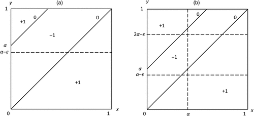
The game in question, illustrated in Figure 1, lives on the unit square ($0\le x\le 1$ and $0\le y\le 1$), having the payoff kernel

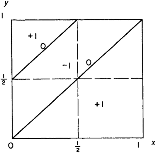
One of the players, the maximizer, chooses x, whereas the other player, the minimizer, chooses y.

Let f and g denote probability measures on the unit interval. We will write $f(M)$ for the probability mass assigned by f to a measurable set $M\subseteq [0,1]$. If $M=\{x_0\}$ is a singleton with $x_0\in [0,1]$, then we will write alternatively $f\{x_0\}$ for the probability mass assigned by f to $x_0$. Analogous notation will be used for g. The lower and the upper values of the game are defined as

respectively. Intuitively, $\underset{¯}{v}$ corresponds to the expected payoff in a sequential setting in which the maximizer moves first by choosing a mixed strategy f, and the minimizer, observing f (but not its pure-strategy realization), moves second by choosing a mixed strategy g. Similarly, $\overline{v}$ corresponds to the expected payoff in an analogous setting in which the minimizer moves first and the maximizer second. As suggested by this interpretation, we certainly have $\overline{v}\ge \underset{¯}{v}$. The game is said to have a value if $\overline{v}=\underset{¯}{v}$.

The definitions of the lower and upper values do not assume that the respective optimization problems admit a solution. If, however, the supremum is attained in the definition of $\underset{¯}{v}$, then the corresponding f is called an optimal strategy for the maximizer. An analogous terminology applies to the minimizer.

Proposition 1

(Sion and Wolfe [27]). The following statements hold:

1. $\underset{¯}{v}=\frac{1}{3}\approx 0.33$, and an optimal strategy for the maximizer is given by $f\left\{0\right\}=f\left\{\frac{1}{2}\right\}=f\left\{1\right\}=\frac{1}{3}$.

2. $\overline{v}=\frac{3}{7}\approx 0.43$, and an optimal strategy for the minimizer is given by $g\left\{\frac{1}{4}\right\}=\frac{1}{7}$, $g\left\{\frac{1}{2}\right\}=\frac{2}{7}$, and $g\left\{1\right\}=\frac{4}{7}$.

Proof.

See Sion and Wolfe [27]. □

Thus, $\underset{¯}{v}<\overline{v}$, that is, the game does not have a value. This fact is remarkable, despite earlier examples of nonexistence (Ville [29], Wald [31]), because the Sion–Wolfe game admits an interpretation in terms of a Colonel Blotto game with two battlefields and a head start for one player (Aspect and Ewerhart [1], Sion and Wolfe [27, pp. 301–302]). The example therefore shows that nonexistence can arise even in games with practical significance.

For the subsequent analysis (especially for Example 1 below), it will be relevant that the maximizer has an alternative optimal strategy given by $f\left\{0\right\}=\frac{1}{3}$ and $f\left\{1\right\}=\frac{2}{3}$. Indeed, if the maximizer uses this mixed strategy, the expected payoff is at least $\frac{1}{3}$, regardless of the minimizer’s choice of y. Similarly, the minimizer has an alternative optimal strategy in which the mass point given by $g\left\{\frac{1}{4}\right\}=\frac{1}{7}$ is slightly shifted up or down. These observations are relevant for our study because, under the assumptions that we are going to impose, the alternative strategies will be available in approximating discretizations, whereas this need not be so for the strategies characterized in Proposition 1.

3. Finite Approximations

This section studies finite approximations of the Sion–Wolfe game. We start with a “canonical” approximation (Subsection 3.1), take the limit (Subsection 3.2), and then explore several alternative approximations (Subsection 3.3).

3.1. A Canonical Approximation

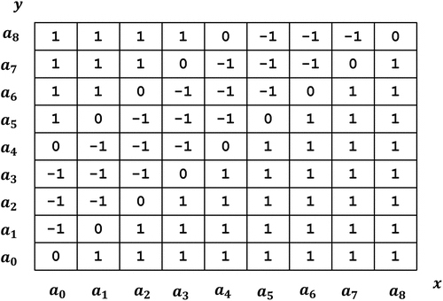
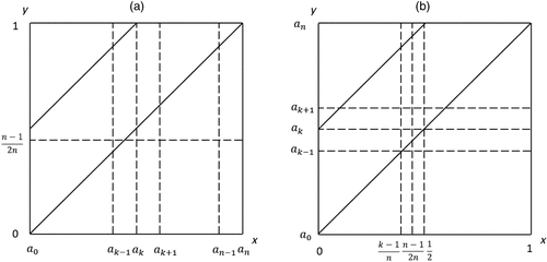
Suppose that the players are restricted to choosing their strategies from a finite, equidistant grid over [0, 1], defined by

where $a_{\nu }=\frac{\nu }{n}$, with $\nu \in \{0,1,\dots ,n\}$, for some positive integer n. Computing payoffs using any approximating kernel $K_n:[0,1]\times [0,1]\to \mathbb{R}$ of the infinite game defines a finite two-person zero-sum game for any n. Because the strategy sets are finite, the supremum and infimum operators in the definition of the game values reduce to the maximum and minimum, respectively. Thus, by von Neumann’s [30] minimax theorem, each finite approximation has a value $v(n)$. Moreover, optimal strategies for maximizer and minimizer exist and are given by probability measures $f_n$ and $g_n$ over the finite grid $\{a_0,\dots ,a_n\}$, respectively. We may then consider the limiting value of the finite approximation, $v_{*}={\lim }_{n\to \infty }v(n)$, provided the limit exists.

The payoff matrix of the finite approximation for $n=8$ and $K_n=K$ is illustrated in Figure 2. In line with the conventions used for the infinite game, we assume that the maximizing player chooses columns and the minimizing player chooses rows. To identify candidate solutions of such games, we found it instructive to apply iterated elimination of weakly dominated strategies (Aspect and Ewerhart [1]). Moreover, at the time of writing, there exists a very convenient web tool that computes the complete solution of a given bimatrix game (Avis et al. [2]). The following proposition characterizes the game value and optimal strategies of the finite approximation with the original kernel in the general case where n is even.

Proposition 2

(Finite Approximation, n Even). Let $n=2k$, for some integer $k\ge 2$. Then,

1. the value of the finite approximation is $v^0(n)=\frac{2}{5}=0.40$;

2. optimal strategies are unique, given for the maximizer by $f_n\left\{a_0\right\}=f_n\left\{a_{k-1}\right\}=\frac{1}{5}$ and $f_n\left\{a_n\right\}=\frac{3}{5}$, and for the minimizer by $g_n\left\{a_{k-1}\right\}=g_n\left\{a_k\right\}=\frac{1}{5}$ and $g_n\left\{a_n\right\}=\frac{3}{5}$.

Proof.

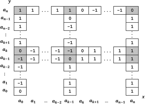
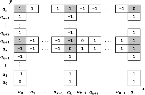
Figure 3 shows the relevant parts of the payoff matrix for $n=2k\ge 4$, where boxes corresponding to outcomes with positive probability in the candidate strategies are shaded. Suppose the minimizer plays $g_n$. Then, any pure strategy $x\in \{a_0,a_{k-1},a_n\}$ yields an expected payoff of $\frac{2}{5}$. Any alternative strategy for the maximizer, be it $x\in \{a_1,\dots ,a_{k-2}\}$, $x=a_k$, or $x\in \{a_{k+1},\dots ,a_{n-1}\}$, is not a best response. Next, suppose that the maximizer plays $f_n$. Then, any $y\in \{a_{k-1},a_k,a_n\}$ yields an expected payoff of $\frac{2}{5}$. Any alternative pure strategy for the minimizer, whether $y=a_0$, $y\in \{a_1,\dots ,a_{k-2}\}$, $y\in \{a_{k+1},\dots ,a_{n-2}\}$, or $y=a_{n-1}$, fails to be a best response. Thus, the game indeed has the value $\frac{2}{5}$. Moreover, by exchangeability, the support of any optimal strategy is contained in $\{a_0,a_{k-1},a_n\}$ for the maximizer and in $\{a_{k-1},a_k,a_n\}$ for the minimizer. As the submatrix of the payoff matrix restricted to these strategies is invertible, optimal strategies are indeed unique. □

3.2. Taking the Limit

The value of the canonical approximation, $v^0(n)=\frac{2}{5}$, remains constant when we raise $n=2k$. Thus, comparing with Proposition 1,

that is, the limiting value of the finite approximations $v_{*}={\lim }_{n\to \infty }v(n)$ lies, in the case of the canonical approximation, strictly inside the interval formed by the lower and upper values of the infinite game.

What about the limit of strategies? The optimal strategies found in Proposition 2 are unique. Moreover, these optimal strategies assign probability $\frac{1}{5}$ to column $x=a_{k-1}$ and row $y=a_{k-1}$ which, for example, become suboptimal when n doubles. As n increases, the strategy $a_{k-1}$ approaches $\frac{1}{2}$, so, regardless of how the limit is taken, the limiting strategy profile in the infinite game loses key qualitative properties of the finite solutions.

A rigorous analysis of the limiting behavior requires the specification of a topology on the space of probability measures. Since Glicksberg [12], it has been standard to use the weak* topology, defined as the coarsest topology that renders all mappings $f\mapsto \int \phi (x)df(x)$ continuous, where $\phi :[0,1]\to \mathbb{R}$ may be any continuous function on the unit interval. If the limit of the approximating strategies is taken with respect to the weak* topology, then the corresponding limit strategies are given as $f\left\{0\right\}=f\left\{\frac{1}{2}\right\}=\frac{1}{5}$ and $f\left\{1\right\}=\frac{3}{5}$ for the maximizer, and by $g\left\{\frac{1}{2}\right\}=\frac{2}{5}$ and $g\left\{1\right\}=\frac{3}{5}$ for the minimizer. These limit strategies are, however, not optimal in the infinite game. Indeed, by choosing $x=0$, the maximizer secures an expected payoff of $\frac{3}{5}>\overline{v}$ against g. Similarly, by choosing $y=1$, the minimizer ensures an expected payoff of $\frac{1}{5}<\underset{¯}{v}$ against f.

Alternatively, one may take the limit in the space of finitely additive probability measures (Yanovskaya [32])¹ equipped with the topology of pointwise convergence. By definition, this is the coarsest topology for which all mappings $f\mapsto f(M)$ are continuous, for any interval $M\subseteq [0,1]$. For instance, the limit set function for the maximizer is characterized by $f\left\{0\right\}=f((\frac{1}{2}-\epsilon ,\frac{1}{2}))=\frac{1}{5}$ for any sufficiently small $\epsilon >0$ and $f\left\{1\right\}=\frac{3}{5}$. The limit of the approximating optimal strategies is not a mixed strategy because the property of $\sigma$-additivity is lost. Indeed,

Thus, the limiting set function is merely finitely additive. As suggested by the discussion so far, this means that it is feasible to place mass arbitrarily close to, but still below, $\frac{1}{2}$. Although this idea may be intuitively appealing, there is a downside of admitting finitely additive set functions. Specifically, as Kindler [17] explains, expected payoffs need not be well defined if both players use such generalized strategies, because the order of integration may matter in the computation of expected payoffs. Intuitively, it is unclear which player wins, and with what probability, if both players bid as close as possible to, but still strictly below, $\frac{1}{2}$.

3.3. Alternative Approximations

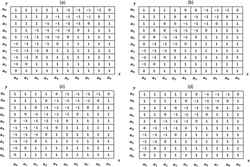
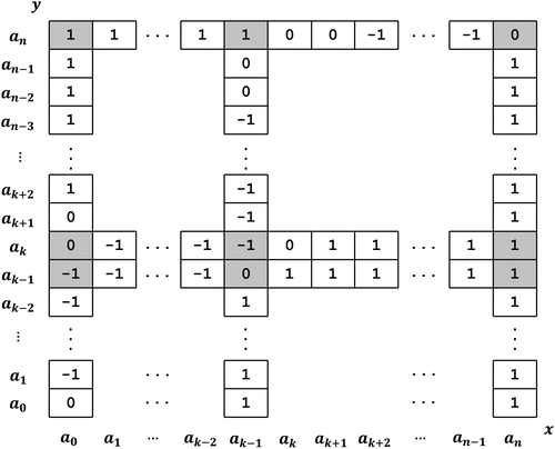
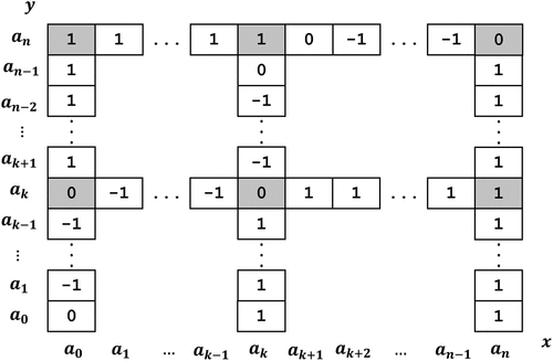
We now consider the case where $n=2k+1$ is odd. Here, identifying a canonical approximation is less straightforward. Figure 4 illustrates a variety of approximations in the case $n=9$ and $k=4$. In panel (a), we depict the payoff matrix in the case in which the original kernel is kept. However, the short diagonal, defined by the set of strategy combinations $(x,y)$ satisfying $y=x+\frac{1}{2}$, vanishes, because when n is odd, there is no solution in the finite lattice. In panels (b) through (d), the original kernel K has been modified to reintroduce the short diagonal. In panel (b), this is done symmetrically. In panels (c) and (d), however, an advantage is given to either the minimizer or the maximizer. Kernels on the unit square extending these examples to general odd $n=2k+1$ are given as follows:

It should be noted that, in contrast to the case where n is even, the kernels defined above may depend on n. In analyzing the approximations for odd n, we focus on the game values, whereas optimal strategies are characterized in the proof.

Proposition 3

(Finite Approximation, n Odd). Let $n=2k+1$ for some integer $k\ge 2$. Then, the respective values of the finite approximations corresponding to kernels $K_n^a$, $K_n^b$, $K_n^c$, and $K_n^d$ are given by $v^a(n)=\frac{3}{7}\approx 0.43$, $v^b(n)=\frac{2}{5}=0.40$, $v^c(n)=\frac{1}{3}\approx 0.33$, and $v^d(n)=\frac{1}{2}=0.50$.

Proof.

For each of the four kernels, referred to below as cases, the proof proceeds by identifying a pair of mutual best responses.

Case a. Suppose that the minimizer selects $g_n\left\{a_k\right\}=\frac{2}{7}$, $g_n\left\{a_{k+1}\right\}=\frac{1}{7}$, and $g_n\left\{a_n\right\}=\frac{4}{7}$. Then, from Figure 5, it is evident that any $x\in \{a_1,\dots ,a_{k-1}\}$ is strictly inferior to $\widehat{x}=a_0$, whereas $x=a_{k+1}$, as well as any $x\in \{a_{k+2},\dots ,a_{n-1}\}$, is strictly inferior to $\widehat{x}=a_n$. Hence, the maximizer’s pure best responses are $a_0$, $a_k$, and $a_n$. Next, suppose that the maximizer selects $f_n\left\{a_0\right\}=\frac{1}{7}$, $f_n\left\{a_k\right\}=\frac{2}{7}$, and $f_n\left\{a_n\right\}=\frac{4}{7}$. Then, $y=a_0$ is strictly inferior to $\widehat{y}=a_k$, and the same is true for any $y\in \{a_1,\dots ,a_{k-1}\}$. In contrast, any $y\in \{a_k,\dots ,a_n\}$ is a best response for the minimizer. In particular, $a_k$, $a_{k+1}$, and $a_n$ are best responses.

Case b. See Figure 6. If the minimizer chooses $g_n\left\{a_{k-1}\right\}=g_n\left\{a_k\right\}=\frac{1}{5}$ and $g_n\left\{a_n\right\}=\frac{3}{5}$, then any $x\in \{a_0,a_{k-1},a_n\}$ yields an expected payoff of $\frac{2}{5}$. Alternative strategies such as $x\in \{a_1,\dots ,a_{k-2}\}$, $x=a_k$, and $x\in \{a_{k+2},\dots ,a_{n-1}\}$ yield a strictly lower expected payoff. The strategy $x=a_{k+1}$ is an alternative best response. If the maximizer chooses $f_n\left\{a_0\right\}=f_n\left\{a_{k-1}\right\}=\frac{1}{5}$ and $f_n\left\{a_n\right\}=\frac{3}{5}$, then any $y\in \{a_{k-1},a_k,a_n\}$ yields an expected payoff of $\frac{2}{5}$. Strategy $y=a_{k+1}$ is an alternative best response for $k\ge 3$ and suboptimal for $k=2$. Other strategies, such as $y\in \{a_0,\dots ,a_{k-2}\}$ and $y\in \{a_{k+2},\dots ,a_{n-1}\}$, are not best responses.

Case c. See Figure 7. If the minimizer selects $g_n\left\{a_k\right\}=\frac{1}{3}$ and $g_n\left\{a_n\right\}=\frac{2}{3}$, then both $x=a_0$ and $x=a_n$ yield an expected payoff of $\frac{1}{3}$. Strategies $x\in \{a_1,\dots ,a_{k-1}\}$ are alternative best responses. The strategy $x=a_k$, as well as any $x\in \{a_{k+1},\dots ,a_{n-1}\}$, is not a best response. If the maximizer chooses $f_n\left\{a_0\right\}=\frac{1}{3}$ and $f_n\left\{a_n\right\}=\frac{2}{3}$, then both $y=a_k$ and $y=a_n$ yield an expected payoff of $\frac{1}{3}$. Strategies $y\in \{a_1,\dots ,a_{k-1}\}$ are alternative best responses. Any other strategy, be it $y=a_0$, $y=a_{k+1}$, or $y\in \{a_{k+2},\dots ,a_{n-1}\}$, is not a best response for the minimizer.

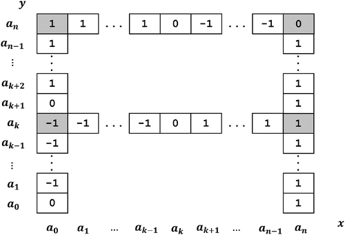
Case d. See Figure 8. If the minimizer selects $g_n\left\{a_k\right\}=g_n\left\{a_n\right\}=\frac{1}{2}$, then any $x\in \{a_0,a_k,a_n\}$ yields an expected payoff of $\frac{1}{2}$. The strategy $x=a_{k+1}$ is an alternative best response, whereas $x\in \{a_1,\dots ,a_{k-1}\}$ and $x\in \{a_{k+2},\dots ,a_{n-1}\}$ yield a strictly lower expected payoff. If the maximizer selects $f_n\left\{a_0\right\}=f_n\left\{a_k\right\}=\frac{1}{4}$ and $f_n\left\{a_n\right\}=\frac{1}{2}$, then both $y=a_k$ and $y=a_n$ yield an expected payoff of $\frac{1}{2}$. Strategies $y\in \{a_1,\dots ,a_{k-1}\}$ and $y\in \{a_{k+1},\dots ,a_{n-2}\}$ are alternative best responses, whereas $y=a_0$ or $y=a_{n-1}$ is not a best response for the minimizer. □

Thus, when the original kernel is kept, corresponding to panel (a) in Figure 4, the value of the finite approximation equals the upper value of the infinite game, that is, $v^a(n)=\overline{v}$. In the unbiased case, corresponding to panel (b), the game value matches the case of even n, lying strictly within the interval formed by the lower and upper values of the infinite game. If the kernel is biased in favor of the minimizer, corresponding to panel (c), we obtain the lower value of the infinite game, that is, $v^c(n)=\underset{¯}{v}$. Somewhat unexpectedly, however, if the kernel is biased toward the maximizer, corresponding to panel (d), the game value of the finite approximation strictly exceeds the upper value of the infinite game, that is,

As mentioned in the introduction, this possibility is undesirable because it implies that values of the finite games do not even allow one to put a bound on infinite-game lower or upper values.

Dasgupta and Maskin [7] noted that the Sion–Wolfe game does not admit an $\epsilon$-equilibrium, for $\epsilon >0$ small enough. However, there is no connection between the failure of the limiting values to correspond to the continuous case and the lack of $\epsilon$-equilibria for the Sion–Wolfe game. Instead, as shown by Tijs [28], the nonexistence of $\epsilon$-equilibria is a general property of two-person zero-sum games that do not have a value. In fact, a two-person zero-sum game has a value if and only if it admits an $\epsilon$-equilibrium for any $\epsilon >0$. In particular, there is no obvious link between the nonexistence of $\epsilon$-equilibria and the anomaly captured by Proposition 3.

4. Discussion

In this section, we examine the observed differences between the finite-game limiting values and the infinite-game lower and upper values. We first derive the solution of the game in which only one player is restricted to choosing from a finite grid (Subsection 4.1). Next, we study the robustness of the Sion–Wolfe game (Subsection 4.2). Finally, we use the insights thereby obtained to examine the anomaly observed in Proposition 3 (Subsection 4.3).

4.1. Restricting One Player’s Strategy Choice

Unlike the previous setup, we now assume that one player’s strategy is restricted to a finite grid, while the other player’s strategy remains unrestricted. Consider first the case where the maximizer is restricted, corresponding to panel (a) of Figure 9. Let n be a positive integer, and let $K_n$ be an approximating kernel, which is henceforth assumed to be measurable and bounded on the unit square. Then,

is the (lower) value of the game in which the maximizer chooses a probability measure $f_n$ over the finite grid $\{a_0,\dots ,a_n\}$, while the minimizer chooses a probability measure g over the unit interval [0, 1]. Similarly, consider the case where the minimizer is restricted, corresponding to panel (b). Then,

is the (upper) value of the game in which the minimizer chooses a probability measure $g_n$ over the finite grid $\{a_0,\dots ,a_n\}$, while the maximizer chooses a probability measure f over the interval [0, 1].

Peck [22] established a general minimax theorem for games in which the strategy set of one player is finite. Although that result assumes that both players choose finitely supported probability measures $f^{\text{fin}}$ and $g^{\text{fin}}$, it still implies that the two games just introduced have a value. For example, for the game in which the maximizer is restricted, we have

which proves the claim. The argument for the game in which the minimizer is restricted is analogous. The relevance for the present study is that the values $\underset{¯}{v}(n)$ and $\overline{v}(n)$ are game values, that is, there are no separate lower- or upper-value counterparts worth studying.

The following result characterizes the solution of these games for $K_n=K$, where attention is restricted to the case of even n.

Proposition 4.

Let $n=2k$, for some integer $k\ge 2$. Then,

1. $\underset{¯}{v}(n)=\frac{1}{3}$, with optimal strategies for the maximizer given by $f_n\left\{a_0\right\}=\frac{1}{3}$ and $f_n\left\{a_n\right\}=\frac{2}{3}$, and for the minimizer by $g\left\{\frac{n-1}{2n}\right\}=\frac{1}{3}$ and $g\left\{1\right\}=\frac{2}{3}$;

2. $\overline{v}(n)=\frac{3}{7}$, with optimal strategies for the maximizer given by $f\left\{0\right\}=\frac{2}{7}$, $f\left\{\frac{n-1}{2n}\right\}=\frac{1}{7}$, and $f\left\{1\right\}=\frac{4}{7}$, and for the minimizer by $g_n\left\{a_{k-1}\right\}=\frac{1}{7}$, $g_n\left\{a_k\right\}=\frac{2}{7}$, and $g_n\left\{a_n\right\}=\frac{4}{7}$.

Proof.

To show part i, suppose the minimizer plays g. Then, as is evident from Figure 9(a), the maximizer’s expected payoff is $\frac{1}{3}$ for any pure strategy $x\in \{a_0,\dots ,a_{k-1}\}$. The same is true for $x=a_k$ and $x=a_n$. In contrast, the expected payoff from any $x\in \{a_{k+1},\dots ,a_{n-1}\}$ is strictly lower. Hence, $f_n$ is a best response to g. Next, assume that the maximizer chooses $f_n$. Then, the expected payoff is $\frac{1}{3}$ for $y\in (0,\frac{1}{2})$ and for $y=1$, whereas the expected payoff is strictly higher for any other choice of $y\in [0,1]$. Hence, g is also a best response to $f_n$. For part ii, see Figure 9(b). If the minimizer chooses $g_n$, then the maximizer’s expected payoff is $\frac{3}{7}$ from pure strategies $x=0$, $x\in (\frac{k-1}{n},\frac{1}{2})$, and $x=1$, whereas the expected payoff is strictly lower for any other pure strategy. Noting that $\frac{n-1}{2n}$ lies strictly between $\frac{k-1}{n}=\frac{n-2}{2n}$ and $\frac{1}{2}=\frac{n}{2n}$, we see that f is a best response to $g_n$. On the other hand, if the maximizer plays f, then the expected payoff is $\frac{3}{7}$ for the pure strategies $y\in \{a_1,\dots ,a_k\}$ and $y=a_n$, whereas the expected payoff is strictly higher otherwise. Thus, $a_{k-1}$, $a_k$, and $a_n$ are best responses for the minimizer, completing the proof. □

These observations are in line with the intuition, reviewed in the previous section, that the outcome of the Sion–Wolfe game hinges on which player will be able to bid closest to, but still below, $\frac{1}{2}$. Specifically, if the maximizer’s choice is restricted to the finite grid, while the minimizer’s choice is unrestricted, then the game value equals the lower value of the Sion–Wolfe game, that is, $\underset{¯}{v}(n)=\underset{¯}{v}$. Intuitively, the maximizer has an incentive to marginally overbid the minimizer’s lower bid, but is unable to do so because $a_{k-1}<\frac{n-1}{2n}<a_k=\frac{1}{2}$, that is, because of the restrictions imposed by the finite grid. However, if the minimizer’s choice is restricted to the finite grid, while the maximizer’s choice is unrestricted, then the game value equals the upper value of the Sion–Wolfe game, that is, $\overline{v}(n)=\overline{v}$. In this case, it is the minimizer who has an incentive to overbid the maximizer’s bid $\frac{n-1}{2n}$, but is unable to do so.

4.2. Robustness of the Sion–Wolfe Game

Consider the kernel

where $\alpha \in (0,1)$ is a parameter that corresponds to the vertical position of the short diagonal. The Sion–Wolfe game has $\alpha =\frac{1}{2}$. In the case $\alpha >\frac{1}{2}$, illustrated in panel (a) of Figure 10, the short diagonal is shifted up compared with the Sion–Wolfe game. An example is $K_n^c$, where $\alpha =\frac{k+1}{n}$. In the case $\alpha <\frac{1}{2}$, illustrated in panel (b), the short diagonal is shifted down. An example is $K_n^d$, where $\alpha =\frac{k}{n}$.

As our next result reveals, the nonexistence of a value in the case $\alpha =\frac{1}{2}$ is an isolated phenomenon. For this, let $\underset{¯}{v}(K_{\alpha })$ and $\overline{v}(K_{\alpha })$ denote the infinite-game lower and upper values associated with the kernel $K_{\alpha }$. It will be useful to describe a continuum of optimal strategies. Specifically, as in the discussion following Proposition 1, this will allow us to choose an optimal strategy from an approximating grid (see Example 2 below).

Proposition 5.

The following statements hold:

1. If $\alpha \in (\frac{1}{2},1)$, then $\underset{¯}{v}(K_{\alpha })=\overline{v}(K_{\alpha })=\frac{1}{3}$, with optimal strategies for the maximizer given by $f\left\{0\right\}=\frac{1}{3}$ and $f\left\{1\right\}=\frac{2}{3}$, and for the minimizer by $g\{\alpha -\epsilon \}=\frac{1}{3}$ and $g\left\{1\right\}=\frac{2}{3}$, for any sufficiently small $\epsilon >0$.

2. If $\alpha \in (\frac{1}{3},\frac{1}{2})$, then $\underset{¯}{v}(K_{\alpha })=\overline{v}(K_{\alpha })=\frac{1}{2}$, with optimal strategies for the maximizer given by $f\left\{0\right\}=f\left\{\alpha \right\}=\frac{1}{4}$ and $f\left\{1\right\}=\frac{1}{2}$, and for the minimizer by $g\{\alpha -\epsilon \}=g\{2\alpha -\epsilon \}=\frac{1}{4}$ and $g\left\{1\right\}=\frac{1}{2}$, for any sufficiently small $\epsilon >0$.

Proof.

For part i, as can be seen from Figure 10(a), f guarantees an expected payoff of $\frac{1}{3}$ for the maximizer. For the minimizer, g ensures that the expected payoff will not exceed $\frac{1}{3}$. For part ii, see Figure 10(b). The strategy f guarantees an expected payoff of $\frac{1}{2}$. Conversely, for the minimizer, using g ensures that the maximizer will never get more than $\frac{1}{2}$. □

Intuitively, for $\alpha >\frac{1}{2}$, the minimizer can announce a randomization between $y=1$ and a bid slightly below $\alpha$, thereby making it impossible for the maximizer to avoid the outcome $-1$ with a bid different from $x=1$. On the other hand, for $\alpha \in (\frac{1}{3},\frac{1}{2})$, the maximizer is in a better position compared with the Sion–Wolfe game. Indeed, the knife-edge strategy $y=\frac{1}{2}$ loses its strategic advantage for the minimizer.

4.3. Conceptual Framework

We now use the insights obtained above to decompose the discrepancy between finite-approximation values and the infinite-game lower/upper values. As before, we start from the Sion–Wolfe game with kernel K. Given an approximating kernel $K_n$ defined on the unit square, let $\underset{¯}{v}(K_n)$ and $\overline{v}(K_n)$ denote the corresponding infinite-game lower and upper values. Further, let $\min \{K_n,K\}$ denote the kernel formed by the pointwise minimum of $K_n$ and K, and let $\underset{¯}{v}(\min \{K_n,K\})$ denote the corresponding lower value. Analogously, let $\max \{K_n,K\}$ denote the kernel formed by the pointwise maximum of $K_n$ and K, and let $\overline{v}(\max \{K_n,K\})$ denote the corresponding upper value.

Proposition 6.

The difference between $v(n)$ on the one hand and $\underset{¯}{v}$ and $\overline{v}$ on the other decomposes into several terms with definite signs, as visualized below:

$$\begin{array}{ccccccccc}& & \overline{v}(n)& & & & \overline{v}\left(\max \{K_n,K\}\right)& & \\ & \le & & \ge & & \le & & \ge & \\ & & & & \overline{v}(K_n)& & & & \overline{v}\\ v(n)& & & & \ge & & & & \le \\ & & & & \underset{¯}{v}(K_n)& & & & \underset{¯}{v}\\ & \ge & & \le & & \ge & & \le & \\ & & \underset{¯}{v}(n)& & & & \underset{¯}{v}\left(\min \{K_n,K\}\right)& & \end{array}$$

Proof.

All inequalities follow immediately from the respective definitions. □

Each of the upper (lower) four inequalities represents a difference term contributing to the discrepancy between $v(n)$ and $\overline{v}$ (between $v(n)$ and $\underset{¯}{v}$). It should be noted that the respective differences all have a simple interpretation and a definite sign. We explain the four terms for the maximizer. First, $\overline{v}(n)-v(n)\ge 0$ is the maximizer’s gain, starting from the finite game, from being able to play an unrestricted strategy. Next, $\overline{v}(n)-\overline{v}(K_n)\ge 0$ is the loss for the maximizer resulting from lifting restrictions on the minimizer’s strategy. Third, $\overline{v}(\max \{K_n,K\})-\overline{v}(K_n)\ge 0$ is the gain in the upper value from replacing the approximating kernel $K_n$ by the modified kernel $\max \{K_n,K\}$ that approximates K from above. Fourth and finally, $\overline{v}(\max \{K_n,K\})-\overline{v}\ge 0$ is the reduction in the upper value from replacing the modified kernel $\max \{K_n,K\}$ by the original kernel K. The terms for the lower values have analogous interpretations.

The logic underlying the proposition above is not entirely new, but extends ideas already contained in Ville [29]. See also Bohnenblust et al. [4] and Ben-El-Mechaiekh and Dimand [3]. Indeed, in the case where the kernel does not depend on n, the right part of the visualization in Proposition 6 collapses. Moreover, the assumption of continuity may be utilized to prove that the four “error terms” $\overline{v}(n)-v(n)$, $\overline{v}(n)-\overline{v}$, $v(n)-\underset{¯}{v}(n)$, and $\underset{¯}{v}-\underset{¯}{v}(n)$ all vanish as $n\to \infty$. Because Ville [29] did not consider kernel approximations, his analysis was necessarily limited to these four terms. Further, for the Sion–Wolfe game, payoffs are not continuous, so that these error terms need not vanish in the limit.

We illustrate the decomposition implied by Proposition 6 with two examples.

Example 1.

For the finite approximation in Proposition 2, we have $K=K_n$, so that $\overline{v}(K_n)=\overline{v}(\max \{K_n,K\})=\overline{v}$ and $\underset{¯}{v}(K_n)=\underset{¯}{v}(\min \{K_n,K\})=\underset{¯}{v}$. From the discussion following Proposition 1, we know that the minimizer has an optimal strategy in the infinite game with mass points at $\frac{1}{2}$, 1, and at some point that may be chosen flexibly from a small neighborhood of $\frac{1}{4}$. Thus, an optimal strategy is available for the restricted minimizer if $n=2k$ is sufficiently large. Therefore, $\overline{v}(n)=\overline{v}(K_n)=\overline{v}$ for large enough n. Similarly, we obtain that $\underset{¯}{v}(n)=\underset{¯}{v}(K_n)=\underset{¯}{v}$. Hence, the limiting value of the finite approximations satisfies $v_{*}\in [\underset{¯}{v},\overline{v}]$.

Example 2.

For the kernel $K_n^d$ introduced before Proposition 3, we have $K_n^d\ge K$, as is evident from Figure 10(b). Therefore, $\overline{v}(K_n^d)=\overline{v}(\max \{K_n^d,K\})$. Moreover, from Proposition 5, we know that $\underset{¯}{v}(K_n^d)=\overline{v}(K_n^d)=\frac{1}{2}$. By the same result, noting that $\alpha =a_k$, an optimal strategy for the maximizer can be found with support contained in the respective finite grid. For the minimizer, we note that an optimal strategy is given by $g\left\{a_{k-1}\right\}=g\left\{a_{n-2}\right\}=\frac{1}{4}$ and $g\left\{a_n\right\}=\frac{1}{2}$. Hence, $\underset{¯}{v}(K_n^d)=\underset{¯}{v}(n)$ and $\overline{v}(K_n^d)=\overline{v}(n)$, which implies that $\underset{¯}{v}(n)=v(n)=\overline{v}(n)$ in this case. Consequently, the driving force behind the anomaly $v_{*}>\overline{v}$ is the bias of the approximating kernel $K_n^d$, whereas all other terms vanish.

In Example 2, the kernel approximation introduced to preserve the qualitative properties of the finite approximation is therefore seen to be the “culprit” behind the anomaly discussed following Proposition 3.

5. Related Literature

As mentioned above, games without a value have been known for a long time. In Ville’s [29] example, players choose numbers from the unit interval to outbid each other, where the payoff from the highest bid is modified to be strictly dominated. Similarly, in Wald’s [31] example, each player chooses a positive integer. The higher number wins, and there is a draw if both players choose the same number. In a recent paper, Holzman [16, p. 2294] showed that a two-player win–lose game, along with all of its subgames, satisfies the minimax property if and only if none of its subgames is isomorphic to a “larger number game.”

A solution to the Sion–Wolfe game and similar games can be obtained by modifying the game. This holds, for example, if one player is restricted to using an absolutely continuous strategy (Parthasarathy [21]), or if players may use probability measures that are not necessarily $\sigma$-additive (Kindler [17], Yanovskaya [32]), or if the payoff function is modified at selected points (Boudreau and Schwartz [5], Simon and Zame [26]). However, these approaches do not constitute a solution to the original game.

Examples of zero-sum games on the square that have some similarity to the Sion–Wolfe game appear in Carmona [6], Duggan [8], Monteiro and Page [19], Prokopovych and Yannelis [23], and Boudreau and Schwartz [5], for instance. However, those papers pursue the more ambitious objective of characterizing better-reply security (Reny [24]) in the mixed extension.

A notable two-person zero-sum game is Silverman’s game (Evans [9], Heuer and Leopold-Wildburger [15]). The variety and depth of the game-theoretic analysis of Silverman’s game contrast with the elementary nature of the present analysis. See, for example, Evans and Heuer [10] and Heuer [14]. However, the conclusions are similar. Indeed, continuous variants of Silverman’s game need not possess a value, although discrete variants may often possess an essentially unique equilibrium.

6. Conclusion

This paper makes two main contributions. First, Propositions 2 and 3 show that the limits of approximating game values in the Sion–Wolfe game convey little information about the lower and upper values of an infinite game. Second, motivated by Propositions 4 and 5, Proposition 6 decomposes the observed differences into several, easily interpretable terms with definite signs. As the discussion of Examples 1 and 2 reveals, in addition to optimal strategies against a restricted or unrestricted opponent potentially not being available in the finite approximation, kernel approximations, whether upward or downward, may have a more substantial impact on limiting values than one might expect. In sum, our findings indicate that caution is required when using finite approximations to predict equilibrium play. Moreover, because Proposition 6 extends to other two-person zero-sum games in a straightforward way, the present paper also provides a flexible tool for analyzing the sources of any discrepancies between finite-game and infinite-game values more generally.

References

- [1] (2022) Colonel Blotto games with a head start. Preprint, submitted September 16, http://dx.doi.org/10.2139/ssrn.4204082.Google Scholar
- [2] (2010) Enumeration of Nash equilibria for two-player games. Econom. Theory 42(1):9–37.Crossref, Google Scholar
- [3] (2010) Von Neumann, Ville, and the minimax theorem. Internat. Game Theory Rev. 12(02):115–137.Crossref, Google Scholar
- [4] (1948) Mathematical theory of zero-sum two-person games with a finite number or a continuum of strategies. Report, RAND Corporation, Santa Monica, CA.Google Scholar
- [5] (2019) A knife-point case for Sion and Wolfe’s game. Working paper, Bagwell Center for the Study of Markets and Economic Opportunity, Kennesaw State University, Kennesaw, GA.Google Scholar
- [6] (2005) On the existence of equilibria in discontinuous games: Three counterexamples. Internat. J. Game Theory 33(2):181–187.Crossref, Google Scholar
- [7] (1986) The existence of equilibrium in discontinuous economic games, I: Theory. Rev. Econom. Stud. 53(1):1–26.Crossref, Google Scholar
- [8] (2007) Equilibrium existence for zero-sum games and spatial models of elections. Games Econom. Behav. 60(1):52–74.Crossref, Google Scholar
- [9] (1979) Silverman’s game on intervals. Amer. Math. Monthly 86(4):277–281.Crossref, Google Scholar
- [10] (1992) Silverman’s game on discrete sets. Linear Algebra Appl. 166:217–235.Crossref, Google Scholar
- [11] (1952) Fixed-point and minimax theorems in locally convex topological linear spaces. Proc. Natl. Acad. Sci. USA 38(2):121–126.Crossref, Google Scholar
- [12] (1952) A further generalization of the Kakutani fixed point theorem, with application to Nash equilibrium points. Proc. Amer. Math. Soc. 3(1):170–174.Google Scholar
- [13] (1990) Subgame perfect equilibrium in continuous games of perfect information: An elementary approach to existence and approximation by discrete games. J. Econom. Theory 52(2):406–422.Crossref, Google Scholar
- [14] (2001) Three-part partition games on rectangles. Theoret. Comput. Sci. 259(1–2):639–661.Crossref, Google Scholar
- [15] (2012) Silverman’s Game: A Special Class of Two-Person Zero-Sum Games (Springer, Berlin).Google Scholar
- [16] (2025) The minimax property in infinite two-person win-lose games. Math. Oper. Res. 50(3):2287–2300.Link, Google Scholar
- [17] (1983) A general solution concept for two-person, zero-sum games. J. Optim. Theory Appl. 40(1):105–119.Crossref, Google Scholar
- [18] (2023) Discrete Colonel Blotto games with two battlefields. Internat. J. Game Theory 52(4):1111–1151.Crossref, Google Scholar
- [19] (2007) Uniform payoff security and Nash equilibrium in compact games. J. Econom. Theory 134(1):566–575.Crossref, Google Scholar
- [20] (1954) On von Neumann’s minimax theorem. Pacific J. Math. 4(1):65–72.Crossref, Google Scholar
- [21] (1970) On games over the unit square. SIAM J. Appl. Math. 19(2):473–476.Crossref, Google Scholar
- [22] (1958) Yet another proof of the minimax theorem. Canadian Math. Bull. 1(2):97–100.Crossref, Google Scholar
- [23] (2014) On the existence of mixed strategy Nash equilibria. J. Math. Econom. 52:87–97.Crossref, Google Scholar
- [24] (1999) On the existence of pure and mixed strategy Nash equilibria in discontinuous games. Econometrica 67(5):1029–1056.Crossref, Google Scholar
- [25] (1987) Games with discontinuous payoffs. Rev. Econom. Stud. 54(4):569–597.Crossref, Google Scholar
- [26] (1990) Discontinuous games and endogenous sharing rules. Econometrica 58(4):861–872.Crossref, Google Scholar
- [27] (1957)
On a game without a value . Contributions to the Theory of Games III, Annals of Mathematics Studies (Princeton University Press, Princeton, NJ), 299–306.Google Scholar - [28] (1977) -equilibrium point theorems for two-person games. Methods Oper. Res. 26:755–766.Google Scholar
- [29] (1938) Applications aux Jeux de Hasard: Cours Professé a la Faculté des Sciences de Paris. Traité du Calcul des Probabilités et de ses Applications: Tome IV, Applications Diverses et Conclusion, Fascicule II (Gauthier-Villars, Paris).Google Scholar
- [30] (1928) Zur Theorie der Gesellschaftsspiele. Math. Ann. 100(1):295–320.Crossref, Google Scholar
- [31] (1945) Generalization of a theorem by v. Neumann concerning zero sum two person games. Ann. Math. 46(2):281–286.Crossref, Google Scholar
- [32] (1970) The solution of infinite zero-sum two-person games with finitely additive strategies. Theory Probab. Its Appl. 15(1):153–158.Crossref, Google Scholar