On the Diameter of the Stopped Spider Process

1. Introduction

We consider the Brownian “spider process,” also known as Walsh Brownian motion, as first introduced in the epilogue of Walsh [18]. Early constructions of Walsh’s Brownian motion were given by Rogers [16] using resolvents, by Baxter and Chacon [3] using infinitesimal generators, and by Salisbury [17] using excursion theory. Barlow et al. [2] considered the construction of Walsh Brownian motion as a process living on $n\ge 1$ rays meeting at a common point (reminiscent of a spider). An explicit connection between Walsh Brownian motion and queueing theory was recently established by Atar and Cohen [1], who considered queue length processes in the form of Walsh Brownian motion.

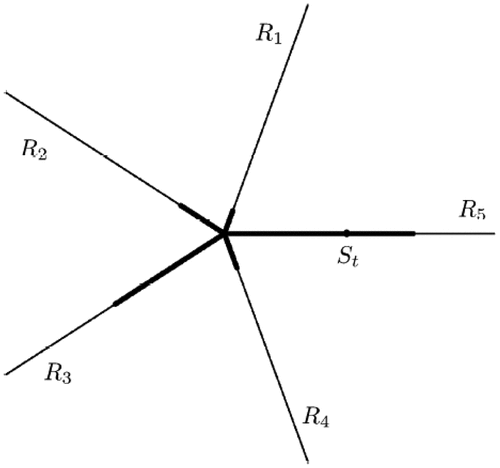
It is the construction of Walsh Brownian motion by Barlow et al. [2] that we shall employ in the present paper. Our main purpose shall be to solve an optimal stopping problem for the spider process to be formulated in Equation (8). Before revealing this optimal stopping problem, we begin with some background and necessary definitions. The construction of the spider process is motivated by the fundamental observation that standard one-dimensional Brownian motion can be viewed as an absolute value of itself, each of whose excursions is assigned a random sign. Following the construction in Barlow et al. [2] and Dubins and Schwarz [4], the spider process, with $n\ge 3$ rays emanating from the origin, may be viewed as the extension of the observation to an n-valued sign. More precisely, for a given positive integer n, consider the collection of n rays $R_k=\{e^{2\pi ik/n}t\hspace{0.17em}:\hspace{0.17em}t\ge 0\},\hspace{0.17em}k=1,\hspace{0.17em}2,\hspace{0.17em}\dots ,\hspace{0.17em}n,$ on the plane. Let $\theta ={({\theta }_m)}_{m\ge 0}$ be the sequence of independent “complex signs” (i.e., the family of random variables with the uniform distribution on $\{e^{2\pi ik/n}:k=1,2,\dots ,n\}$). Assume further that $B={(B_t)}_{t\ge 0}$ is a Brownian motion independent of θ, and let $e={(e_t)}_{t\ge 0}$ be the associated excursion process (see Revuz and Yor [13, chapter XII]). The set of excursions is countable, and hence, it can be ordered by the set of natural numbers. The spider process S is then given by $S_t={\theta }_{m(t)}|B_t|$, where m(t) is the number of the excursion of B, which straddles t (see Revuz and Yor [13, p. 488]). From this definition, we see that for the case n = 1, the spider process reduces to reflecting Brownian motion $|B|$; the case n = 2 corresponds to standard Brownian motion.

The optimal stopping problem in (8) is motivated by the development of optimal bounds for the expected “size” (as defined in Equations (4) and (5)) of the stopped spider process. For a given $t\ge 0$ and $\omega \in \mathrm{\Omega }$, let $T_t(\omega )$ denote the trajectory up to time t:

Moreover, let $d_t(\omega )$ stand for the sum of the deviations of $T_t(\omega )$ along the rays: that is,

We shall sometimes refer to these deviations as the “ribs” of S.

L. E. Dubins wished to design a stopping time to maximize the coverage of Brownian motion on the spider for a given expected time (see Ernst [6, p. 487]). That is, Dubins sought to find the best constant c_n such that

for any integrable stopping time τ of S (i.e., measurable with respect to the filtration generated by the spider process). We refer to this problem as the Dubins’ “spider problem.” This problem has been solved only in the cases n = 1 and n = 2. When n = 1, $S=|B|$, and hence, (3) becomes

Dubins and Schwarz [4] proved that the value $c_1=\sqrt{2}$ is optimal; one may also consult Dubins et al. [5] for an alternative approach. Other related literature includes Gilat et al. [7, 8] and Meilijson [11]. For n = 2, the spider process reduces to standard Brownian motion, and we define d to be the difference of the running maximum and the running minimum, namely

In Dubins et al. [5], the authors proved that the optimal choice for c₂ is equal to $\sqrt{3}$. For $n\ge 3$, a tempting conjecture is that $c_n=\sqrt{n+1}$, but this appears to not be so, at least for n = 3 (see Ernst [6]).

In this work, we solve a version of Dubins’ spider problem in which the coverage or size of the spider process is measured differently. In this formulation, we shall replace d_t by the diameter D_t with respect to the British rail metric: that is, for n = 1, we have

For $n\ge 2$, we have

In other words, $D_t(\omega )$ is given as in (2), but only one or two largest summands are taken into account (depending, respectively, on whether n = 1 or $n\ge 2$). In the simpler case that $n\in \{1,2\}$, then d_t = D_t, and so, the optimal constant C_n in the inequality

equals $\sqrt{2}$ for n = 1 and equals $\sqrt{3}$ for n = 2. The key purpose of the present paper is to identify the optimal value of C_n for $n\ge 3$. We preview our main result as Theorem 1, which shall be proved in Section 4. The asymptotics of the constants C_n are addressed in Theorem 2.

Theorem 1.

For $n\ge 3$, the best constant in (6) is given by

$$C_n=2\sqrt{U(0,0,0)},$$

where $U(0,0,0)$ is defined in Corollary 3.

A few remarks concerning the general strategy for proving our main result are now in order. By a straightforward time-homogeneity argument, it suffices to find the optimal constant κ_n in the inequality

Indeed, it follows from the scaling properties of Brownian motion that for any fixed $\lambda >0,\hspace{0.17em}{({\tilde{S}}_t^{\lambda })}_{t\ge 0}={(\lambda S_{t/{\lambda }^2})}_{t\ge 0}$ is a spider process, and for any integrable stopping time of S, ${\tilde{\tau }}^{\lambda }=\tau {\lambda }^2$ is a stopping time of $\tilde{S}$. Consequently, applying the inequality to ${\tilde{S}}^{\lambda }$ with the corresponding diameter $\tilde{D}$, we obtain

Optimizing over λ, we obtain

which is the desired inequality. To see that the constant is optimal, we will construct an integrable stopping time for which equality holds in (7); because $\mathbb{E}\tau +{\kappa }_n\ge 2\sqrt{{\kappa }_n\mathbb{E}\tau }$, this will immediately show that τ is also optimal for (6).

The estimate (7) leads directly to the optimal stopping problem

where the supremum is taken over all integrable stopping times τ of S. Given an optimal stopping problem, we may generalize the problem to the case in which the underlying Markov process is allowed to start from an arbitrary point in the associated state space. As a result, the corresponding value $\mathbb{U}$ extends to the value (or “reward”) function on the entire state space. This object has many structural properties, which in many cases, enable its explicit identification (and which in turn, yield the solution to the initial optimal stopping problem). To find the reward function, we typically exploit one of the following two strategies.

1. Using Markovian arguments, we write a system of differential equations that the value function should satisfy. Then, applying analytic arguments and exploiting homogeneity in the problem structure (if there is any), we attempt to solve the system and guess the “right” function.

2. We attempt to guess the optimal strategy. To do so, we compute the value function by specifying for each starting point the corresponding optimal stopping time.

Sometimes, a successful solution requires a clever combination of both (A) and (B). It should be emphasized that both these approaches typically only yield the candidate for the reward function (during the search and the construction for the reward function, one usually exploits a number of guesses and/or some additional assumptions, which are not a priori guaranteed). Next, having found the candidate, one proceeds to rigorous proof and checks the excessiveness and optimality of the constructed function. If both excessiveness and optimality hold, then the candidate coincides with the value function, and the optimal stopping problem is solved.

In solving the optimal stopping problem in (8), we shall exploit both strategies (A) and (B). We shall also rely on the theory of martingale inequalities, which have proven essential in many areas of operations research (see, for example, Karr [10] and Rhee and Talagrand [14, 15]). We will also need a number of novel arguments; in particular, in order to reduce dimensionality and represent the spider process in terms of a relatively simple Markovian structure, we shall employ a skew Brownian motion with jumps. Furthermore, by a certain translation property and an appropriate reduction trick (both to be revealed in Section 2), we shall see that the analysis of the optimal stopping problem in (8) shall heavily depend on the solution of a related auxiliary two-dimensional optimal stopping problem in (9) for a standard Brownian motion.

The remainder of this paper is organized as follows. Section 2 is concerned with the analysis of the aforementioned auxiliary stopping problem in (9). For the sake of completeness, we also present the solution to the optimal stopping problem in (8) for the cases n=1 and n=2. Although the solution for both these cases has already appeared in the literature, we find that their analyses provide helpful intuition about the optimal strategy for the general case. Section 3 is devoted to the construction of the candidate for the value function for $n\ge 3$. It is the most technically innovative part of the paper; our efforts shall include the aforementioned reduction as well as a combination of arguments from methods (A) and (B). Section 4 proves that the constructed candidate coincides with the desired value function and then, shows how the optimal stopping problem in (8) leads to the proof of our main result in Theorem 1.

2. Preparation

2.1. A Related Optimal Stopping Problem

We begin with a problem, which itself is not new (see, for example, Ernst [6]) but whose analysis will be quite helpful for the present paper. For the sake of convenience and clarity, we split the reasoning into several intermediate steps.

Step 1.

Suppose that $X={(X_t)}_{t\ge 0}$ is a standard one-dimensional Brownian motion, and denote by $Y={(Y_t)}_{t\ge 0}$ the associated one-sided maximal function (i.e., $Y_t={\sup }_{0\le s\le t}{X}_s$ for $t\ge 0$). Consider the optimal stopping problem

where the supremum is taken over all integrable stopping times τ of X. By Wald’s identity, the time variable can be removed; the supremum equals $\mathbb{V}=\sup \mathbb{E}(Y_{\tau }-X_{\tau }^2)$, thus giving rise to the optimal stopping problem for the Markov process (X, Y). We define the associated state space asand we introduce the gain function $G:\mathcal{D}\to \mathbb{R}$ given by $G(x,y)=y-x^2$. We then have the identitywhich fits into the general framework of the theory of optimal stopping (see, for example, Peskir and Shiryaev [12]). As mentioned in the previous section, a successful treatment of (10) requires the generalization of the problem to the case in which the process (X, Y) starts from an arbitrary point in the state space $\mathcal{D}$. This is standard; one first extends the process (X, Y) to a Markov family on $\mathcal{D}$, introducing the family of initial distributions ${({\mathbb{P}}_{x,y})}_{(x,y)\in \mathcal{D}}$ given by the requirement that, for all $(x,y)\in \mathcal{D}$,

Next, one defines the associated value function

where the supremum is taken over all ${\mathbb{P}}_{x,y}$-integrable stopping times τ of X. Alternatively, one can define $\mathbb{V}(x,y)$ using a single probability measure ${\mathbb{P}}_{0,0}$ bywhere the supremum is taken over all ${\mathbb{P}}_{0,0}$-integrable stopping times τ of X.

Step 2.

Following the usual approach from general optimal stopping theory (see, for example, Peskir and Shiryaev [12]), we split the state space $\mathcal{D}$ into two sets: the continuation region C and the instantaneous stopping region D. They are given, respectively, by

Thus, to solve (11) (and hence, also (10)), one needs to identify the shape of the continuation region and the formula for $\mathbb{V}$ on this set. Having done that, the optimal stopping time is given by

Standard Markovian arguments (see Peskir and Shiryaev [12, chapter 3]) indicate that $\mathbb{V}$ should be in C¹ and should satisfy the following requirements

Note that Equations (14) and (15) arise from the application of the generator of the Markov process (X, Y) to the function $\mathbb{V}$; (16) is the consequence of the principle of smooth fit.

Step 3.

The key geometric properties of the continuation and stopping sets arise from the following arguments. First, we observe that by (12),

where in the second line, we have used the identity ${\mathbb{E}}_{0,0}{X}_{\tau }=0$. This yields the following translation property of C; if $(x,y)\in C$ and $\lambda \ge -y$, then $(x+\lambda ,y+\lambda )\in C$. Indeed, if $\mathbb{V}(x,y)>G(x,y)$, we have

By passing to the complement, D enjoys the same translation property. The second observation is that if $(x,y)\in D$ and $y\prime >y$, then $(x,y\prime )$ also lies in the stopping region. Indeed, if $a,\hspace{0.17em}b,\hspace{0.17em}c\in \mathbb{R}$ satisfy the inequality b < c, then

and so, for any stopping time τ, we have the inequality

Taking the supremum over all τ, we obtain that $\mathbb{V}(x,y\prime )\le G(x,y\prime )$, which implies that $(x,y\prime )\in D$. Combining the two observations, we see that there is a constant a > 0 such that

and

Note that the use of strict/nonstrict inequalities comes from the fact that C is open and D is closed. This is because of the continuity of $\mathbb{V}$ and G.

Step 4.

Now, based on (14)–(16), we provide the formula for the candidate for the value function, which will be denoted by V. By (14) and (16), we see that if (x, y) lies in the continuation set, then

Applying the condition in (15) yields $a=\frac{1}{2}$. We have thus obtained that

Step 5.

It is straightforward to see that the function V obtained is excessive (that is, it satisfies (14)–(16)). Hence, by applying Itô’s formula, we have that $V\ge \mathbb{V}$. The reverse inequality is obtained by considering the stopping time given in (13). This stopping time is integrable, even exponentially (see, for example, Wang [19]). Furthermore, for any $(x,y)\in \mathcal{D}$, the stopped process $(X^{\tau },Y^{\tau })$ evolves along the continuation region, and Itô’s formula gives

This proves that $V=\mathbb{V}$. We pause to note that the optimal stopping time in (13) has the following interpretation. If the distance between X and Y is less than $\frac{1}{2}$, it is beneficial to wait; otherwise, we should stop. This strategy makes intuitive sense as well. If X is near its running maximum, then there is a high probability that the maximum will increase at any given moment (thus, increasing the value $\mathbb{V}$), and the cost of waiting, expressed in terms of time or the increase of $\mathbb{E}{X}^2$, is relatively small. However, when the distance is large, it may take longer for X to return to Y, so the expected cost of waiting is too high; hence, it is optimal to stop immediately. These heuristics shall prove helpful in the sequel.

2.2. On (8) for n = 1

We now proceed with the study of the spider process. In the case n = 1, the process coincides with the reflecting Brownian motion $|X|={(|X_t|)}_{t\ge 0}$. Let Y denote the corresponding two-sided maximal function

Recalling (8) and invoking Wald’s identity lead us to the optimal stopping problem

where the supremum is taken over all integrable stopping times τ of $|X|$. The analysis essentially proceeds along the same lines as in the previous subsection. Because the maximal function Y is two sided, we modify the domain to $\mathcal{D}=\{(x,y):|x|\le y\}$, introduce the value functionand define the continuation and stopping regions C and D by the same formulas as before. Note that $G(x,y)=G(-x,y)$ and that the distribution of (X, Y) under ${\mathbb{P}}_{x,y}$ is the same as that of $(-X,Y)$ under ${\mathbb{P}}_{-x,y}$. We thus conclude that

The key difference here is that the presence of two-sided maximal function disables Equation (17), which had proven to be fundamental in the previous analysis.

To overcome this difficulty, we present the following reduction argument, which shows that $\mathbb{U}$ and $\mathbb{V}$ coincide on a large part of the domain. First, because Y is not smaller than the one-sided maximal function, the direct comparison of the formulas for $\mathbb{U}$ and $\mathbb{V}$ gives that $\mathbb{U}\ge \mathbb{V}$ on $\mathcal{D}$. Next, suppose that y₀ is a nonnegative number such that $(0,y_0)\in D$. Repeating the reasoning from Step 3, we see that the entire half-line

is contained within D. Thus, for any $x\ge 0$, in the definition of $\mathbb{U}(x,y_0)$ one can restrict oneself to those stopping times τ for which the process $X^{\tau }$ does not go below zero; indeed, for other stopping times, the process $(X^{\tau },Y^{\tau })$ crosses the line $\mathcal{\ell }$, which is not optimal (see (13)). However, for such τ, the process Y coincides with the one-sided maximal function, and hence, by the very definition of $\mathbb{U}$ and $\mathbb{V}$, we have the desired reverse bound $\mathbb{U}(x,y_0)\le \mathbb{V}(x,y_0)$. This in particular implies that $y_0\ge \frac{1}{2}$ because otherwise, we would obtaina contradiction. Denoting by b the infimum of all y₀’s, we have that for $y\ge b$,

We now apply Markovian arguments to obtain ${\mathbb{U}}_{xx}=0$ on C; one also may note that by the symmetry condition in (19), we have that, for y < b,

These two observations imply that the function $\mathbb{U}$ must be constant on $\mathcal{D}\cap \{y<b\}$, and by continuity, $\mathbb{V}$ must be constant on the line segment $[0,b]\times \{b\}$. This implies that $b=\frac{1}{2}$, leading us to the construction of the candidate function

It is straightforward to check that U is excessive and hence, that $U\ge \mathbb{U}$; the reverse bound is obtained by considering the stopping time in (13). The optimal strategy is to wait until the distance between $|X|$ and its running maximum is at least $\frac{1}{2}$. Intuitively, this remains perfectly consistent with the strategy for the previous problem.

2.3. The case n = 2

Here, the analysis will be a more involved, but again, the special function $\mathbb{V}$ will play a prominent role.

Step 1.

The spider process S coincides with the standard one-dimensional Brownian motion, which we shall denote again by X. Let $Y={(Y_t)}_{t\ge 0}$ and $Z={(Z_t)}_{t\ge 0}$ be the running maximum and the running infimum of X; that is, for $t\ge 0$,

and

Motivated by (8) and Wald’s identity, we introduce the optimal stopping problem

where the supremum is taken over all integrable stopping times τ of X. It is important to note that, in contrast to the previous considerations, there are now three variables involved.

To apply the general theory of optimal stopping, we extend the triple (X, Y, Z) to a Markov family on the state space

Let the corresponding family of initial distributions be denoted by ${({\mathbb{P}}_{x,y,z})}_{(x,y,z)\in \mathcal{D}}.$ Having done so, we introduce the gain function $G(x,y,z)=y-z-x^2$ and the value function

Here, the supremum is taken over all ${\mathbb{P}}_{x,y,z}$-integrable stopping times τ of X. The associated continuation and the instantaneous stopping regions are given by

and the optimal stopping time in (21) is

Step 2.

We now provide an initial comparison of the functions $\mathbb{U}$ and $\mathbb{V}$, exploiting a similar argument as in the case n = 1. We begin with the observation that both the inequalities $Y_{\tau }\ge y$ and $Z_{\tau }\le z$ hold ${\mathbb{P}}_{x,y,z}$ almost surely. This implies that

and

By the definition of $\mathbb{U}$ and $\mathbb{V}$, (24) gives

To see the consequence of (25), note that, under ${\mathbb{P}}_{x\prime ,y,z},\hspace{0.17em}(X,-Z)$ has the same distribution as (X, Y) under ${\mathbb{P}}_{-x,-z,-y}$. We, therefore, obtain

Indeed, both (26) and (27) can be reversed on a large part of the domain. Let $z<0<y$ be fixed numbers, and suppose that there is $x\in (z,y)$ such that the state (x, y, z) belongs to the stopping domain. Then, the whole half-line

is entirely contained within D (repeating the argument from Step 3). Next, suppose that $x\prime >x$. Then, in the definition of $\mathbb{U}(x\prime ,y,z)$, it is enough to consider only those stopping times τ for which the process ${(X^{\tau })}_{t\ge 0}$ does not go below x. Indeed, for other stopping times, the process $(X^{\tau },Y^{\tau },Z^{\tau })$ crosses the line $\mathcal{\ell }$, which is not optimal (see (23)). However, for such τ, the running infimum $Z^{\tau }$ will not change, so

An analogous argument works for $x\prime <x$; in this case, when studying (21), one may restrict oneself to stopping times τ for which $X^{\tau }$ does not go above x, which keeps $Y^{\tau }$ fixed and yields the desired reverse identity

Step 3.

Note that (26) and (27) imply that if $y-z<1$, then $(x,y,z)\in C$ for all $x\in [z,y]$. Indeed, for any such x, we have $x-z<\frac{1}{2}$ or $y-x<\frac{1}{2}$, and hence, $\mathbb{V}(x,y)>y-x^2$ or $\mathbb{V}(x,-z)\ge -z-x^2$. This gives

It is useful to note that this in perfect consistence with the optimal strategies described at the end of the previous two subsections; if $y-z<1$, then the distance between x and y or the distance between x and z is less than $\frac{1}{2}$, and hence, it is beneficial to wait. This observation also suggests what to do if $y-z\ge 1$. If both x – z and y – x are at least $\frac{1}{2}$, one should stop; otherwise, wait. In other words, by the analysis carried out in the previous step, we obtain that the candidate U for the value function satisfies, if $y-z\ge 1$,

For $y-z<1$, one exploits Markovian arguments and obtains the system of equations

This system can be solved explicitly (see Dubins et al. [5] and Ernst [6]) (see also Section 3); we obtain

Step 4.

The analysis is completed by showing that $U=\mathbb{U}$. This is done as we have done so previously; one checks that U is excessive, and hence, $U\ge \mathbb{U}$. The reverse bound follows from the construction because U is obtained by exercising the optimal strategy described. We omit the details, instead referring the interested reader to Dubins et al. [5] and Ernst [6].

3. On the Search for the Value Function for $n\ge 3$

Equipped with the machinery and intuition, we proceed to the analysis of the case n = 3. The purpose of this section is to obtain a candidate U for the value function associated with the appropriate optimal stopping problem. The reasoning rests on a number of guesses and assumptions that may (at least at first glance) seem imprecise. However, the reader should keep in mind that our purpose in this part of the manuscript is only to guess an appropriate special function. The necessary rigorous analysis will be presented in Section 4. Again, for purposes of clarity, we split the reasoning into intermediate steps.

Step 1

First, we need to specify the underlying Markov process, which will be subject to the optimal stopping procedure. Of course, we could consider the process

where X takes the values inand $Y_t^{(j)}$ measures the length of jth rib up to time t, but this process has a rather complicated structure. Fortunately, there is an alternative for which the state space is simpler: a three-dimensional structure. As a starting point, note that the diameter of the spider process depends only on the behavior of two longest ribs, and hence, as it was for n = 2, it is natural to attempt to find some representation of S on the real line. For $t\ge 0$, let us distinguish the longest rib by(where $T_t(\omega )$ was defined in (1)), and let $-Z_t$ (note the minus sign) be the corresponding second-longest rib, so that $D_t=Y_t-Z_t$. Now, to define X, we first set $|X_t|$ to be the distance of the spider process S_t from the origin. Furthermore, if S_t belongs to the “running longest rib,” we assume that $X_t\ge 0$; otherwise, we assume that X is negative. In other words, we copy the running longest rib on the positive half-line, whereas all the remaining ribs are glued together and copied on $(-\infty ,0]$. For a graphical illustration of the arguments, see Figure 2.

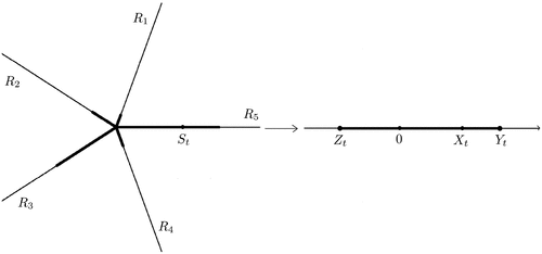
The process X can be interpreted in the language of skew Brownian motion (see, for example, Harrison and Shepp [9]). Given $\alpha \in [0,1]$, the α-skew Wiener process can be obtained from reflecting Brownian motion by changing (independently) the sign of each excursion with probability α. Thus, 0-skew Wiener process is reflecting Brownian motion, whereas $\frac{1}{2}$-skew Wiener process is the usual Brownian motion. The α-skew Wiener process behaves like the usual Wiener process except for the asymmetry at the origin; if located at zero, then for any s > 0, the process has probability α of reaching –s before s.

Note that the process X defined is a $1-n^{-1}$-skew Brownian motion, which possesses the additional jump part; if for a given t > 0, its left limit $X_{t-}$ equals $-Y_t$, then X_t changes its sign, moving to Y_t. This discontinuity (or “phase transition”) corresponds to the scenario in which the second-longest rib becomes the longest.

Step 2

We now gather some basic information about the behavior of the triple (X, Y, Z). It is straightforward to check that this is a time-homogeneous, right-continuous strong Markov process on the state space

As usual, we shall denote by ${({\mathbb{P}}_{x,y,z})}_{(x,y,z)\in \mathcal{D}}$ the corresponding family of initial distributions such that

We now discuss the action of the associated infinitesimal generator $\mathbb{L}$. Let f be a bounded sufficiently regular function on E. If x > 0, then up to time $\tau =\inf \{t:X_t=0\}$, the process Z is constant, and the pair (X, Y) behaves as the Brownian motion along with its maximal function. Consequently, we have $\mathbb{L}f(x,y,z)=\frac{1}{2}{f}_{xx}(x,y,z)$; furthermore, the maximal function component enforces the condition $f_y(y,y+,z)=0$ (see Peskir and Shiryaev [12, p. 134] for a related calculation). Similarly, if x < 0 and $z>-y$, then $\mathbb{L}f(x,y,z)=\frac{1}{2}{f}_{xx}(x,y,z)$, and one has to impose the requirement $f_z(z,y,z-)=0$. If x = 0, then X behaves locally like the $1-n^{-1}$-skew Brownian motion, so $\mathbb{L}f(0,y,z)=\frac{1}{2}{f}_{xx}(0+,y,z)$, and we need to assume $f_{xx}(0-,y,z)=f_{xx}(0+,y,z)$ and $(1-n^{-1})f_x(0-,y,z)=n^{-1}{f}_x(0+,y,z)$ (see Revuz and Yor [13, p. 292]). Finally, if $x=z=-y$, then X changes its sign instantly; we have $X_t>0$ almost surely for any t > 0, with ${\lim }_{t\to 0}{X}_t=-x$. Therefore, we may write

Now, by the analysis, the first ratio on the right converges to $\mathbb{L}f(-x,y,z)$ as $t\to 0$, and hence, the existence of the limit defining $\mathbb{L}f(x,y,z)$ enforces the additional condition $f(-y,y,-y)=f(y,y,-y)$ for all y. Summarizing, we have shown that the generator of (X, Y, Z) acts via $\frac{1}{2}\frac{{\partial }^2}{\partial x^2}$ on the space of bounded continuous functions f on E, such that f_xx exists for $x\ne 0$, and we have

for all $y,\hspace{0.17em}z$, and $f(-y,y,-y)=f(y,y,-y)$ for all y.

Step 3

We continue with the properties of (X, Y, Z). It is immediate that the process enjoys the following Brownian scaling.

Lemma 1.

For any $\lambda >0$, the process

$$t\mapsto (\lambda X_{t{\lambda }^{-1/2}},\lambda Y_{t{\lambda }^{-1/2}},\lambda Z_{t{\lambda }^{-1/2}})$$

has the same law under ${\mathbb{P}}_{x,y,z}$ as does (X, Y, Z) under ${\mathbb{P}}_{\lambda x,\lambda y,\lambda z}$.

We will also need the following property.

Lemma 2.

Let y < 1/2 and $\sigma =\inf \{t>0:Y_t\ge 1/2\}$. Then, the distribution of $Z_{\sigma }$ under ${\mathbb{P}}_{x,y,z}$ is determined by

$${\mathbb{P}}_{x,y,z}(Z_{\sigma }\le s)=\{\begin{array}{ll}0\hfill & if \hspace{0.17em}s<-\frac{1}{2},\hfill \\ \frac{(n-1)(1-2x)}{n-1-2s}\hfill & if \hspace{0.17em}x\ge 0,\hspace{0.17em}-y\le s<z,\hfill \\ \frac{n-1-2x}{n-1-2s}\hfill & if \hspace{0.17em}x<0,\hspace{0.17em}-y\le s<z,\hfill \\ \frac{(n-1)(1+2s)}{n-1-2s}\hfill & if \hspace{0.17em}-\frac{1}{2}\le s<-y,\hfill \\ 1\hfill & if \hspace{0.17em}s\ge z.\hfill \end{array}$$

Proof.

It suffices to prove the formula for $-\frac{1}{2}\le s<z$ because for the remaining s, the claim is obvious. We consider three separate cases.

Case 1.

Suppose that $x\ge 0$ and $y\ge -s$. By the law of total probability,

$${\mathbb{P}}_{x,y,z}(Z_{\sigma }>s)=2x+(1-2x){\mathbb{P}}_{0,y,z}(Z_{\sigma }>s).$$(28)

The equation contains two disjoint scenarios. The process X may visit 1/2 before it visits 0; this occurs with probability 2x and automatically implies that $Z_{\sigma }>s$. The second possibility is that X drops to 0 before it reaches 1/2. Then, no matter how much Y has increased, the set $\{Z_{\sigma }>s\}$ has conditional probability ${\mathbb{P}}_{0,y,z}(Z_{\sigma }>s)$; indeed, the latter does not depend on the value of $y\in [-s,1/2)$. To compute this probability, note that because $y\ge -s$, we have

$${\mathbb{P}}_{0,y,z}(Z_{\sigma }>s)={\mathbb{P}}_{-s,y,z}(Z_{\sigma }>s)/n.$$(29)

The inequality $Z_{\sigma }>s$ means that when X reaches –s, the spider process is on the longest rib; by symmetry, the probability of this scenario is $1/n$. After that, no matter how much Z has dropped, the event $\{Z_{\sigma }>s\}$ occurs with the conditional probability equal to ${\mathbb{P}}_{-s,y,z}(Z_{\sigma }>s)$. Now, applying (28) with $x=-s$, we obtain that

$${\mathbb{P}}_{0,y,z}(Z_{\sigma }>s)=-2s/(n-1-2s)$$

or

$${\mathbb{P}}_{0,y,z}(Z_{\sigma }\le s)=\frac{n-1}{n-1-2s}.$$

Plugging this into (28) yields

$${\mathbb{P}}_{x,y,z}(Z_{\sigma }\le s)=\frac{(n-1)(1-2x)}{n-1-2s}.$$

Case 2.

Next, assume that x < 0 and $y\ge -s$. The inequality $Z_{\sigma }>s$ implies that X must rise to zero before it drops to s. The change in Z is irrelevant, so

$${\mathbb{P}}_{x,y,z}(Z_{\sigma }>s)=\left(1-\frac{x}{s}\right){\mathbb{P}}_{0,y,z}(Z_{\sigma }>s)=\frac{2(x-s)}{n-1-2s}.$$

Case 3.

Finally, suppose that $y<-s$. Then, conditioning on the time at which X first visits –s, we obtain

$${\mathbb{P}}_{x,y,z}(Z_{\sigma }>s)={\mathbb{P}}_{-s,-s,z}(Z_{\sigma }>s).$$

Again, the drop in Z is not important, and we may write z in the lower index on the right. Hence,

$${\mathbb{P}}_{x,y,z}(Z_{\sigma }\le s)={\mathbb{P}}_{-s,-s,z}(Z_{\sigma }\le s)=\frac{(n-1)(1+2s)}{n-1-2s},$$

where the latter equality follows from the analysis in Case 1. □

Step 4

We proceed to the study of the optimal stopping problem in (8). As before, we extend it to an arbitrary starting point $(x,y,z)\in \mathcal{D}$, setting

whereand the supremum is taken over all integrable stopping times τ of X (indeed, the Wald identity $\mathbb{E}{X}_{\tau }^2=\mathbb{E}\tau$ remains valid because ${(|X_t|)}_{t\ge 0}$, denoting the distance of S from the origin, is the reflected Brownian motion). Markovian arguments and the discussion in Step 2 show that $\mathbb{U}$ satisfies the following system of equations:

As a direct consequence of (31), the stopping set has the property that if it contains two points of the form (x, y, z) and $(x\prime ,y,z)$, then it also automatically contains the entire line segment that joins these two points. Otherwise, by the concavity of the function $x\mapsto G(x,y,z)$, this would violate the inequality $\mathbb{U}\ge G$.

Step 5

Our construction for the candidate U for the value function will be based on the guess of the optimal stopping strategy. Equipped with the analysis in the case n = 2, a naive idea is to try to proceed analogously (i.e., consider the optimal stopping times τ, which consist of two stages).

• Stage 1. Wait until the difference between Y and Z is equal to one.

• Stage 2. Wait until Y – X and X – Z are both larger than $\frac{1}{2}$.

Some thought reveals that this cannot be the optimal strategy. To see this, suppose that the first stage is over, and then, after some time, we have X = 0 and $Z\in (-\frac{1}{2},0)$. Because of the asymmetry of the skew Brownian at zero (which in our case, “pushes” the process on the negative side), the cost of waiting for X to reach Z is lower than in the symmetric case, so the margin $\frac{1}{2}$ should be increased, at least if at the end of Stage 1 we have X = Z.

On the other hand, it is natural to expect that the strategy is not far from optimal. It seems plausible to try the following general two-step procedure.

• Stage 1. Wait until Y and Z become “distant.”

• Stage 2. Wait until $f(Y,Z)\le X\le g(Y,Z)$ for some functions f and g.

Note that in the light of the arguments, we must have $Y-Z>1$ and hence, $Y>\frac{1}{2}$ at the end of the first stage (we have $Y\ge -Z$ almost surely).

Step 6

We now turn to the study of some basic properties of f and g. First, note that f depends only on z and g depends only on y. The idea behind this is as follows. Suppose that $(x,y,z)\in D$; then, $(x,y\prime ,z)$ and $(x,y,z\prime )$ also lie in the stopping set, provided $y\prime >y$ and $z\prime <z$ (the argument is the same as in the case n = 2). So, when computing $\mathbb{U}(z,y,z)$, we may restrict ourselves to those stopping times τ for which X does not cross f(y, z); for such τ, the process $Y^{\tau }$ is constant, and hence, for $x<f(y,z)$, we have

The problem thus reduces to the optimal stopping of X and Z. The stopping boundary cannot depend on y, and hence, $f(Y,Z)=f(Z)$. We can now go one step further; if $f(z)\le 0$, then for τ, $-Z^{\tau }$ is the one-sided maximal function of $-X^{\tau }$. Hence,

and so, in particular, $f(z)=z+\frac{1}{2}$. A similar argument shows that $g(Y,Z)=g(Y)$; however, because $y>\frac{1}{2}$ (see the end of the previous step), we obtain $g(y)=y-\frac{1}{2}$ for all y.

Step 7

Now, we will find the formula for f for z close to zero (so that f(z) > 0). To this end, we will show that f satisfies an appropriate ordinary differential equation. We thus fix such a z. By (31), (34), and the principle of smooth fit,

We obtain the identity

Applying (33), we have that

Note the initial condition $f(-\frac{1}{2})=0$, which comes from the case $z\le -\frac{1}{2}$ considered above. This differential equation can be easily solved; the substitution $z=\phi (s)=f^{-1}(s)$ transforms it into the linear equation

whose explicit solution is

Hence, for $z>-\frac{1}{2}$, f is the inverse to the above function. It is not difficult to show that $\phi (1)>0$. This is done by applying the estimate $e^{-x}\ge 1-x+x^2/3$, valid for $x\in [0,1]$, to $x=2/(n-1)$. This implies that $f(0)<1$, and hence,

Step 8

We are now ready to guess the final form of the optimal strategy. We have already constructed appropriate lower and upper boundary functions f and g. Taking the discussion into account, we formulate the procedure as follows.

• Stage 1. Wait until the equality $f(Z)\le g(Y)$ is observed for the first time.

• Stage 2. Wait until $f(Z)\le X\le g(Y)$.

The remaining part of the analysis is devoted to the explicit evaluation of the value function associated with this strategy. In other words, we shall henceforth set

where τ is given as the combination of Stage 1 and Stage 2 above. The discussion we have already carried out gives the following (partial) formula for U.

Corollary 1.

If $y\ge 1/2$ and $z\le \phi (y-\frac{1}{2})$, then

$$U(x,y,z)=\{\begin{array}{ll}y-z-2\left(z+\frac{1}{2}\right)x+{\left(z+\frac{1}{2}\right)}^2\hfill & if \hspace{0.17em}x\le {\phi }^{-1}(z)\le 0,\hfill \\ y-z-\frac{2{\phi }^{-1}(z)}{n-1}x+{({\phi }^{-1}(z))}^2\hfill & if \hspace{0.17em}x\le 0\le {\phi }^{-1}(z),\hfill \\ y-z-2{\phi }^{-1}(z)x+{({\phi }^{-1}(z))}^2\hfill & if \hspace{0.17em}0\le x\le {\phi }^{-1}(z),\hfill \\ y-z-x^2\hfill & if \hspace{0.17em}{\phi }^{-1}(z)\le x\le y-\frac{1}{2},\hfill \\ y-z-2\left(y-\frac{1}{2}\right)x+{\left(y-\frac{1}{2}\right)}^2\hfill & if \hspace{0.17em}x\ge y-\frac{1}{2}.\hfill \end{array}$$(37)

It remains to find the formula for U for $z>\phi (y-\frac{1}{2})$. We consider the cases $y\ge \frac{1}{2}$ and $y<\frac{1}{2}$ separately.

Step 9

First, we study the case $y\ge \frac{1}{2}$; this is the most difficult part. We begin with a formula for U_y.

Lemma 3.

Let $y\ge 1/2$ and $z>\phi (y-\frac{1}{2})$. The function U satisfies

$$U_y(x,y,z)=\{\begin{array}{ll}\frac{(n-1)(y-x)}{(n-1)y-\phi (y-\frac{1}{2})}\hfill & if \hspace{0.17em}x\ge 0,\hfill \\ \frac{(n-1)y-x}{(n-1)y-\phi (y-\frac{1}{2})}\hfill & if \hspace{0.17em}x\le 0.\hfill \end{array}$$(38)

Proof.

It suffices to prove the formula for $x\ge 0$; indeed, by Markovian arguments, we see that U satisfies (31) and (34) (with $\mathbb{U}$ replaced by U), so

$$U(x,y,z)=\{\begin{array}{ll}U(0,y,z)+U_x(0-,y,z)x\hfill & \text{if} \hspace{0.17em}x\le 0,\hfill \\ U(0,y,z)+(n-1)U_x(0-,y,z)x\hfill & \text{if} \hspace{0.17em}x\ge 0\hfill \end{array}$$

and

$$U_y(x,y,z)=\{\begin{array}{ll}{U}_y(0,y,z)+U_{xy}(0-,y,z)x\hfill & \text{if} \hspace{0.17em}x\le 0,\hfill \\ U_y(0,y,z)+(n-1)U_{xy}(0-,y,z)x\hfill & \text{if} \hspace{0.17em}x\ge 0.\hfill \end{array}$$

Hence, if (38) is valid for $x\ge 0$, it automatically holds for x < 0 as well.

Therefore, we shall henceforth assume that $x\ge 0$. Our plan is to write

$$U_y(x,y+,z)=\underset{\delta \downarrow 0}{\lim }\frac{U(x,y+\delta ,z)-U(x,y,z)}{\delta }$$(39)

and to analyze the expectations defining $U(x,y,z)$ and $U(x,y+\delta ,z)$. To this end, we fix a small $\delta >0$ (so that $z\ge \phi (y+\delta -\frac{1}{2})$) and consider the events

$$\begin{array}{ll}{A}_1\hfill & =\{\text{the}\hspace{0.17em}\text{trajectory}\hspace{0.17em}\text{of}\hspace{0.17em}X\hspace{0.17em}\text{reaches}\hspace{0.17em}y+\delta \hspace{0.17em}\text{before}\hspace{0.17em}\phi (y+\delta -1/2)\},\hfill \\ A_2\hfill & =\{\text{the}\hspace{0.17em}\text{trajectory}\hspace{0.17em}\text{of}\hspace{0.17em}X\hspace{0.17em}\text{reaches}\hspace{0.17em}\phi (y+\delta -1/2)\hspace{0.17em}\text{before}\hspace{0.17em}y\},\hfill \\ A_3\hfill & =\{\text{the}\hspace{0.17em}\text{trajectory}\hspace{0.17em}\text{of}\hspace{0.17em}X\hspace{0.17em}\text{reaches}\hspace{0.17em}y\hspace{0.17em}\text{before}\hspace{0.17em}\phi (y+\delta -1/2)\hfill \\ \hfill & \hspace{1em}\hspace{1em}\text{but} \text{after} \text{that} \text{reaches}\hspace{0.17em}\phi (y+\delta -1/2)\hspace{0.17em}\text{before}\hspace{0.17em}y+\delta \},\hfill \end{array}$$

Of course A₁, A₂, A₃ are pairwise disjoint, and their union has probability 1. Now, we write

$$U(x,y+\delta ,z)={\mathbb{E}}_{x,y+\delta ,z}(Y_{\tau }-Z_{\tau }-X_{\tau }^2)=I_1+I_2,$$

where

$$I_1={\mathbb{E}}_{x,y+\delta ,z}((Y_{\tau }-Z_{\tau }-X_{\tau }^2)1_{A_1}),\hspace{1em}\hspace{1em}{I}_2={\mathbb{E}}_{x,y+\delta ,z}((Y_{\tau }-Z_{\tau }-X_{\tau }^2)1_{A_1^c}),$$

where $A_1^c=\mathrm{\Omega }\backslash A_1$ is the complement of A₁. By the Markov property, we see that

$$\begin{array}{ll}{I}_2\hfill & ={\mathbb{E}}_{x,y+\delta ,z}((Y_{\tau }-Z_{\tau }-X_{\tau }^2)|A_1^c){\mathbb{P}}_{x,y+\delta ,z}(A_1^c)\hfill \\ \hfill & =U\left(\phi \left(y+\delta -\frac{1}{2}\right),y+\delta ,\phi \left(y+\delta -\frac{1}{2}\right)\right)·\frac{(n-1)(y+\delta -x)}{(n-1)(y+\delta )-\phi (y+\delta -\frac{1}{2})}.\hfill \end{array}$$(40)

We write down a similar splitting for U as $U(x,y,z)=J_1+J_2+J_3$, with

$$J_k={\mathbb{E}}_{x,y,z}((Y_{\tau }-Z_{\tau }-X_{\tau }^2)1_{A_k}),\hspace{1em}\hspace{1em}k=1,\hspace{0.17em}2,\hspace{0.17em}3.$$

A crucial observation is that

$$\begin{array}{ll}{I}_1={\mathbb{E}}_{x,y+\delta ,z}((Y_{\tau }-Z_{\tau }-X_{\tau }^2)1_{A_1})\hfill & ={\mathbb{E}}_{x,y,z}((Y_{\tau }\vee (y+\delta )-Z_{\tau }-X_{\tau }^2)1_{A_1})\hfill \\ \hfill & ={\mathbb{E}}_{x,y,z}((Y_{\tau }-Z_{\tau }-X_{\tau }^2)1_{A_1})=J_1\hfill \end{array}$$

because $Y_{\tau }\ge y+\delta$ on A₁ (by the very definition of this event). Furthermore, arguing as in (40), we obtain

$$J_2=U\left(\phi \left(y+\delta -\frac{1}{2}\right),y,\phi \left(y+\delta -\frac{1}{2}\right)\right)·\frac{(n-1)(y-x)}{(n-1)y-\phi (y+\delta -\frac{1}{2})}.$$

Finally, in order to more easily work with J₃, we rewrite A₃ as the intersection of the following two events:

$$\begin{array}{ll}{A}_3^1\hfill & =\{\text{the} \text{trajectory} \text{of} \hspace{0.17em}X\hspace{0.17em}\text{reaches}\hspace{0.17em}y\hspace{0.17em}\text{before}\hspace{0.17em}\text{reaching}\hspace{0.17em}\phi (y+\delta -1/2)\},\hfill \\ A_3^2\hfill & =\{\text{having}\hspace{0.17em}\text{visited}\hspace{0.17em}y,\hspace{0.17em}\text{the}\hspace{0.17em}\text{trajectory}\hspace{0.17em}\text{of}\hspace{0.17em}X\hspace{0.17em}\text{reaches}\hspace{0.17em}\phi (y+\delta -\frac{1}{2})\hspace{0.17em}\text{before} \text{reaching}\hspace{0.17em}y+\delta \}.\hfill \end{array}$$

Then, using the Markov property, we compute that

$$\begin{array}{ll}\hfill & {\mathbb{E}}_{x,y,z}((Y_{\tau }-Z_{\tau }-X_{\tau }^2)1_{A_3})={\mathbb{E}}_{x,y,\phi (y+\delta -1/2)}((Y_{\tau }-Z_{\tau }-X_{\tau }^2)1_{A_3^1\cap A_3^2})\hfill \\ \hfill & ={\mathbb{E}}_{y,y,\phi (y+\delta -1/2)}((Y_{\tau }-Z_{\tau }-X_{\tau }^2)1_{A_3^2}){\mathbb{P}}_{x,y,z}(A_3^1)\hfill \\ \hfill & ={\mathbb{E}}_{y,y,\phi (y+\delta -1/2)}((Y_{\tau }-Z_{\tau }-X_{\tau }^2)1_{A_3^2})\left[1-\frac{(n-1)(y-x)}{(n-1)y-\phi (y+\delta -1/2)}\right].\hfill \end{array}$$

To analyze the latter expectation, note that on the set $A_3^2$, when X gets to $\phi (y+\delta -\frac{1}{2})$, the value of Y lies between y and $y+\delta$. Consequently,

$$\begin{array}{ll}\hfill & {\mathbb{E}}_{y,y,\phi (y+\delta -1/2)}((Y_{\tau }-Z_{\tau }-X_{\tau }^2)1_{A_3^2})\hfill \\ \hfill & =U\left(\phi \left(y+\delta -\frac{1}{2}\right),y,\phi \left(y+\delta -\frac{1}{2}\right)\right)·\frac{(n-1)\delta }{(n-1)(y+\delta )-\phi (y+\delta -\frac{1}{2})}+o(\delta ).\hfill \end{array}$$

Plugging all this into (39), we obtain

$$U_y(x,y+,z)=\underset{\delta \downarrow 0}{\lim }\frac{I_1+I_2-(J_1+J_2+J_3)}{\delta }=\underset{\delta \downarrow 0}{\lim }\left(\frac{I_2-J_2}{\delta }-\frac{J_3}{\delta }\right).$$

We also have the identity

$$\begin{array}{l}\underset{\delta \downarrow 0}{\lim }\frac{I_2-J_2}{\delta }=\frac{\partial }{\partial w}\left[U\left(\phi \left(y-\frac{1}{2}\right),w,\phi \left(y-\frac{1}{2}\right)\right)\frac{(n-1)(w-x)}{(n-1)w-\phi (y-\frac{1}{2})}\right]{|}_{w=y}\hfill \\ =U_y\left(\phi \left(y-\frac{1}{2}\right),y,\phi \left(y-\frac{1}{2}\right)\right)\frac{(n-1)(y-x)}{(n-1)y-\phi (y-\frac{1}{2})}\hfill \\ \hspace{1em}+U\left(\phi \left(y-\frac{1}{2}\right),y,\phi \left(y-\frac{1}{2}\right)\right)\frac{\partial }{\partial w}\left[\frac{(n-1)(w-x)}{(n-1)w-\phi (y-\frac{1}{2})}\right]{|}_{w=y}.\hfill \end{array}$$

We have already computed (see (37)) that

$$U_y\left(\phi \left(y-\frac{1}{2}\right),y,\phi \left(y-\frac{1}{2}\right)\right)=1.$$

Furthermore, it is straightforward to check that the term

$$U\left(\phi \left(y-\frac{1}{2}\right),y,\phi \left(y-\frac{1}{2}\right)\right)\frac{\partial }{\partial w}\left[\frac{(n-1)(w-x)}{(n-1)w-\phi (y-\frac{1}{2})}\right]{|}_{w=y}$$

is precisely ${\lim }_{\delta \downarrow 0}{J}_3/\delta$. Combining all of the arguments, we obtain the desired claim. This concludes the proof. □

Lemma 3 allows us to extend the formula for U to the domain

$$\left\{(x,y,z):y\ge 1/2,\hspace{0.17em}z>\phi \left(y-\frac{1}{2}\right)\right\},$$

which shall be done in Corollary 2.

Corollary 2.

If $y\ge 1/2$ and $z>\phi \left(y-\frac{1}{2}\right)$, then

$$U(x,y,z)=\{\begin{array}{ll}U\left(x,f(z)+\frac{1}{2},z\right)-{\displaystyle {\int }_y^{f(z)+1/2}\frac{(n-1)(s-x)\text{d}s}{(n-1)s-\phi (y-\frac{1}{2})}}\hfill & if \hspace{0.17em}x\ge 0,\hfill \\ U\left(x,f(z)+\frac{1}{2},z\right)-{\displaystyle {\int }_y^{f(z)+1/2}\frac{((n-1)s-x)\text{d}s}{(n-1)s-\phi (y-\frac{1}{2})}}\hfill & if \hspace{0.17em}x\le 0.\hfill \end{array}$$

Step 10

This is the final part, concerning the case y < 1/2, and it is much simpler. If we denote $\sigma =\inf \left\{t\ge 0:Y_t=\frac{1}{2}\right\}$, then the Markov property gives

To compute the latter expectation, we apply Lemma 2 and immediately obtain the following.

Corollary 3.

If x < 0 and y < 1/2, then we have

$$\begin{array}{ll}U(x,y,z)\hfill & =U\left(\frac{1}{2},\hspace{0.17em}\frac{1}{2},-y\right)·\frac{2((n-1)y-x)}{n-1+2y}+U\left(\frac{1}{2},\hspace{0.17em}\frac{1}{2},z\right)·\frac{2(x-z)}{n-1-2z}\hfill \\ \hfill & +{\displaystyle {\int }_{-1/2}^{-y}U\left(\frac{1}{2},\hspace{0.17em}\frac{1}{2},s\right)}·\frac{2n(n-1)}{{(n-1-2s)}^2}\text{d}s+{\displaystyle {\int }_{-y}^{z}U\left(\frac{1}{2},\hspace{0.17em}\frac{1}{2},s\right)}·\frac{2(n-1-2x)}{{(n-1-2s)}^2}\text{d}s.\hfill \end{array}$$(41)

For $x\ge 0$ and y < 1/2, we compute that

$$\begin{array}{ll}\hfill & U(x,y,z)\hfill \\ \hfill & =U\left(\frac{1}{2},\hspace{0.17em}\frac{1}{2},-y\right)·\frac{2(n-1)(y-x)}{n-1+2y}+U\left(\frac{1}{2},\hspace{0.17em}\frac{1}{2},z\right)·\frac{2((n-1)x-z)}{n-1-2z}\hfill \\ \hfill & \hspace{1em}+{\displaystyle {\int }_{-1/2}^{-y}U}\left(\frac{1}{2},\hspace{0.17em}\frac{1}{2},s\right)·\frac{2n(n-1)}{{(n-1-2s)}^2}\text{d}s+{\displaystyle {\int }_{-y}^{z}U\left(\frac{1}{2},\hspace{0.17em}\frac{1}{2},s\right)}·\frac{2(n-1)(1-2x)}{{(n-1-2s)}^2}\text{d}s.\hfill \end{array}$$(42)

The values of $U(\frac{1}{2},\frac{1}{2},s)$ can be extracted from Corollary 2. In particular, Equation (42) can be applied for $x=y=z=0$, resulting in quite an involved yet nonetheless explicit expression:

It turns out that $3/4\le U(0,0,0)\le 2$ for all n. More precise asymptotics of this constant will be discussed in Theorem 2.

Remark 1.

It is straightforward to check that, for all y > 0, the function U satisfies the symmetry condition $U(-y,y,-y)=U(y,y,-y)$. Compare the first and fifth lines in (37), and see also (41) and (42). This is in perfect consistence with the jump property of X described at the end of Step 1. Indeed, as we noted there, when the left limit $X_{t-}$ is equal to $-Y_t$, then at time t, the process X jumps from $-Y_t$ to Y_t. In other words, the points $(-y,y,-y)$ and $(y,y,-y)$ in the state space correspond to the same value of U.

4. Proof of Theorem 1

We now will prove that the function U constructed in the previous section is indeed the value function of the optimal stopping problem in (8). We begin with the majorization property.

Lemma 4.

For all (x, y, z), we have that

$$U(x,y,z)\ge y-z-x^2.$$

Proof.

Suppose first that $y\ge \frac{1}{2}$ and $z\le \phi (y-\frac{1}{2})$. According to (37), we need to consider five cases. For $x\le {\phi }^{-1}(z)\le 0$, the desired estimate is equivalent to ${(2x-z-1)}^2\ge 0$. If $x\le 0\le {\phi }^{-1}(z)$, then

$$U(x,y,z)=y-z-\frac{2{\phi }^{-1}(z)}{n-1}x+{({\phi }^{-1}(z))}^2\ge y-z\ge y-z-x^2.$$

For $0\le x\le {\phi }^{-1}(z)$, the claim reads ${(x-{\phi }^{-1}(z))}^2\ge 0$. If ${\phi }^{-1}(z)\le x\le y-\frac{1}{2}$, then the majorization is actually an equality. Finally, for $x\ge y-\frac{1}{2}$, the desired bound becomes ${(x-y+\frac{1}{2})}^2\ge 0$, which is also trivial.

Now, suppose that $y<\frac{1}{2}$ or $z>\phi (y-\frac{1}{2})$. It follows directly from (38), (41), and (42) that $U_y(x,y+,z)\le 1$: that is,

$$\frac{\partial }{\partial y+}(U(x,y,z)-(y-z-x^2))\le 0.$$

The majorization follows at once from the analysis; we have

$$U(x,y,z)-(y-z-x^2)\ge U\left(x,{\phi }^{-1}(z)+\frac{1}{2},z\right)-\left({\phi }^{-1}(z)+\frac{1}{2}-z-x^2\right)\ge 0.\hspace{1em}\square$$

Lemma 5.

For any (x, y, z) and any bounded stopping time τ, we have

$${\mathbb{E}}_{x,y,z}(Y_{\tau }-Z_{\tau }-X_{\tau }^2)\le U(x,y,z).$$(44)

Proof.

Roughly speaking, the argument rests on Itô’s formula and the majorization established in the previous section. However, because the function U is not in C², there are some technical obstacles, which will be handled by an appropriate stopping procedure. For sake of clarity, we shall split the reasoning into intermediate parts.

• Part 1. By continuity, we may assume that y > 0 and $-y<z<0$. We introduce the increasing sequences ${({\tau }_n)}_{n\ge 0},{({\sigma }_n)}_{n\ge 0}$ of stopping times given inductively as follows. Let ${\tau }_0\equiv 0$, and for $n\ge 0$,

  $${\tau }_{2n+1}=\inf \left\{t\ge {\tau }_{2n}:X_t=0\hspace{0.17em} \text{or} \hspace{0.17em}{Y}_t\ge \frac{1}{2}\right\},\hspace{1em}{\tau }_{2n+2}=\inf \{t\ge {\tau }_{2n+1}:X_t\in \{Y_t,Z_t\}\}.$$

  Furthermore, let

  $${\sigma }_0=\inf \left\{t\ge 0:Y_t\ge \frac{1}{2}\right\},$$
  and for $n\ge 0$,
  $${\sigma }_{2n+1}=\inf \{t\ge {\sigma }_{2n}:X_t=0\},\hspace{1em}\hspace{1em}{\sigma }_{2n+2}=\inf \{t\ge {\sigma }_{2n+1}:X_t\in \{Y_t,Z_t\}\}.$$

  Here, we use the convention $\inf \varnothing =+\infty$. It is straightforward to see that ${\lim }_{n\to \infty }{\tau }_n={\sigma }_0$ and ${\lim }_{n\to \infty }{\sigma }_n=\infty$ almost surely. The function U is of class $C^{\infty }$ on

  $$D\cap \{(x,y,z):x\ne 0\hspace{0.17em} \text{and} \hspace{0.17em}y<1/2\},$$
  and it satisfies $U_{xx}(x,y,z)=0$ on this set. We may easily check that for all values of y and z,
  $$U_y(y,y,z)=U_z(z,y,z)=0.$$

  Further, for all values of y,

  $$U(-y,y,-y)=U(y,y,-y).$$

  Consequently, by Itô’s formula, we have

  $${\mathbb{E}}_{x,y,z}U(X_{\tau \wedge {\tau }_1},Y_{\tau \wedge {\tau }_1},Z_{\tau \wedge {\tau }_1})=U(x,y,z)$$
  (note that the symmetry condition $U(-y,y,-y)=U(y,y,-y)$ guarantees that the jumps of X do not contribute). Next, on the time interval $[{\tau }_1,{\tau }_2]$, the processes Y and Z remain unchanged, so X behaves like an $1-n^{-1}$-skew Brownian motion there. However, the function $U(·,y_0,z_0)$ satisfies
  $$U_x(0-,y_0,z_0)=(n-1)U_x(0+,y_0,z_0)$$
  and is linear on the intervals $[z_0,0]$ and $[0,y_0]$. This implies
  $${\mathbb{E}}_{x,y,z}U(X_{\tau \wedge {\tau }_2},Y_{\tau \wedge {\tau }_2},Z_{\tau \wedge {\tau }_2})={\mathbb{E}}_{x,y,z}U(X_{\tau \wedge {\tau }_1},Y_{\tau \wedge {\tau }_1},Z_{\tau \wedge {\tau }_1})=U(x,y,z).$$

  Iterating the procedure, we obtain that for any n,

  $${\mathbb{E}}_{x,y,z}U(X_{\tau \wedge {\tau }_n},Y_{\tau \wedge {\tau }_n},Z_{\tau \wedge {\tau }_n})=U(x,y,z).$$

  Hence, letting $n\to \infty$ and applying Lebesgue’s dominated convergence theorem, we get

  $${\mathbb{E}}_{x,y,z}U(X_{\tau \wedge {\sigma }_0},Y_{\tau \wedge {\sigma }_0},Z_{\tau \wedge {\sigma }_0})=U(x,y,z).$$

• Part 2. If $X_{\tau \wedge {\sigma }_0}>0$, then we consider the restriction $U^{+}=U{|}_{{\mathcal{D}}^{+}}$, where ${\mathcal{D}}^{+}=\mathcal{D}\cap \{x\ge 0\}$. Then, $U^{+}(·,y_0,z_0)$ is concave for any $y_0,\hspace{0.17em}{z}_0$ and satisfies $U_y^{+}(y_0,y_0,z_0)=0$. Itô’s formula then gives

  $$\begin{array}{ll}{\mathbb{E}}_{x,y,z}[U(X_{\tau \wedge {\sigma }_1},Y_{\tau \wedge {\sigma }_1},Z_{\tau \wedge {\sigma }_1})|{\mathcal{F}}_{\tau \wedge {\sigma }_0}]\hfill & ={\mathbb{E}}_{x,y,z}[U^{+}(X_{\tau \wedge {\sigma }_1},Y_{\tau \wedge {\sigma }_1},Z_{\tau \wedge {\sigma }_1})|{\mathcal{F}}_{\tau \wedge {\sigma }_0}]\hfill \\ \hfill & \le U^{+}(X_{\tau \wedge {\sigma }_0},Y_{\tau \wedge {\sigma }_0},Z_{\tau \wedge {\sigma }_0})\hfill \\ \hfill & =U(X_{\tau \wedge {\sigma }_0},Y_{\tau \wedge {\sigma }_0},Z_{\tau \wedge {\sigma }_0}).\hfill \end{array}$$

  If $X_{\tau \wedge {\sigma }_0}<0$ (which happens only if $y\ge 1/2$ and $x\le 0$), we may proceed similarly. Consider the restriction $U^{-}=U{|}_{{\mathcal{D}}^{-}}$, where ${\mathcal{D}}^{-}=\mathcal{D}\cap \{x\le 0\}$. Then, $U^{-}(·,y_0,z_0)$ is concave for any $y_0,\hspace{0.17em}{z}_0$, satisfies $U_y^{-}(z_0,y_0,z_0)=0$, and

  $$U^{-}(-y_0,y_0,-y_0)=U^{+}(y_0,y_0,y_0).$$

  Therefore, applying Itô’s formula (and noting that the latter identity allows us to ignore the jumps of X), we obtain again that

  $${\mathbb{E}}_{x,y,z}[U(X_{\tau \wedge {\sigma }_1},Y_{\tau \wedge {\sigma }_1},Z_{\tau \wedge {\sigma }_1})|{\mathcal{F}}_{\tau \wedge {\sigma }_0}]\le U(X_{\tau \wedge {\sigma }_0},Y_{\tau \wedge {\sigma }_0},Z_{\tau \wedge {\sigma }_0}).$$

  Consequently, we have shown that

  $${\mathbb{E}}_{x,y,z}U(X_{\tau \wedge {\sigma }_1},Y_{\tau \wedge {\sigma }_1},Z_{\tau \wedge {\sigma }_1})={\mathbb{E}}_{x,y,z}U(X_{\tau \wedge {\sigma }_0},Y_{\tau \wedge {\sigma }_0},Z_{\tau \wedge {\sigma }_0}).$$

• Part 3. Now, we essentially repeat the reasoning used at the end of Part 1. On the time interval $[{\sigma }_1,{\sigma }_2]$, the processes Y and Z remain unchanged. The function $U(·,y_0,z_0)$ is concave and satisfies

  $$U_x(0-,y_0,z_0)=(n-1)U_x(0+,y_0,z_0).$$

  Consequently, we obtain

  $${\mathbb{E}}_{x,y,z}U(X_{\tau \wedge {\sigma }_2},Y_{\tau \wedge {\sigma }_2},Z_{\tau \wedge {\sigma }_2})\le {\mathbb{E}}_{x,y,z}U(X_{\tau \wedge {\sigma }_1},Y_{\tau \wedge {\sigma }_1},Z_{\tau \wedge {\sigma }_1}).$$

  Iterating the arguments, we see that the sequence

  $${({\mathbb{E}}_{x,y,z}U(X_{\tau \wedge {\sigma }_n},Y_{\tau \wedge {\sigma }_n},Z_{\tau \wedge {\sigma }_n}))}_{n\ge 0}$$
  is nonincreasing and hence, ${\mathbb{E}}_{x,y,z}U(X_{\tau \wedge {\sigma }_n},Y_{\tau \wedge {\sigma }_n},Z_{\tau \wedge {\sigma }_n})\le U(x,y,z).$ By Lemma 5, this implies
  $${\mathbb{E}}_{x,y,z}(Y_{\tau \wedge {\sigma }_n}-Z_{\tau \wedge {\sigma }_n})\le U(x,y,z)+{\mathbb{E}}_{x,y,z}{X}_{\tau \wedge {\sigma }_n}^2\le U(x,y,z)+{\mathbb{E}}_{x,y,z}{X}_{\tau }^2,$$
  where in the final inequality, we have exploited the submartingale property of X². Letting $n\to \infty$, we see that the left-hand side tends to ${\mathbb{E}}_{x,y,z}(Y_{\tau }-Z_{\tau })$ by Lebesgue’s monotone convergence theorem. This yields the desired claim. □

Together with the reasoning from the previous section, Lemma 5 identifies the explicit formula for the value function $\mathbb{U}$ of the optimal stopping process in (30). Corollary 4 thus immediately follows.

Corollary 4.

We have $\mathbb{U}=U$ on D.

We now present the proof of our main result.

Proof of Theorem 1.

Let us write $\mathbb{P}$ instead of ${\mathbb{P}}_{0,0,0}$. By Lemma 5, for any stopping time τ, we have

$$\mathbb{E}(Y_{\tau }-Z_{\tau })\le U(0,0,0)+\mathbb{E}{X}_{\tau }^2=U(0,0,0)+\mathbb{E}\tau .$$

Therefore, a scaling argument discussed in the introductory section yields

$$\mathbb{E}(Y_{\tau }-Z_{\tau })\le 2\sqrt{U(0,0,0)\mathbb{E}\tau },$$

which is the desired inequality. The equality is attained for the special stopping time τ considered in the previous section. Let us first prove that τ is integrable. Consider the auxiliary stopping time

$$\sigma =\inf \left\{t:\underset{0\le s\le t}{\sup }|X_s|\ge \frac{3}{2}\hspace{0.17em} \text{and}|X_t|=\underset{0\le s\le t}{\sup }|X_s|-\frac{1}{2}\right\},$$

which describes the following strategy; we wait until the reflecting Brownian motion reaches the level 3/2 and then, experiences a drop of size 1/2 when compared with its (current) maximal function. Such stopping times are integrable; this follows at once from the results of Dubins et al. [5]. However, it follows directly from the analysis in the previous section that $\tau \le \sigma$ almost surely. Indeed, suppose that at the end of Stage 1, we have X_t = Y _t; then, the estimate (36) implies that

$$X_t=Y_t=Y_t-\frac{1}{2}+\frac{1}{2}=f(Z_t)+\frac{1}{2}<1+\frac{1}{2}=\frac{3}{2}.$$

Then, at the remaining part of the time interval $[0,\tau ]$, we wait until $Y-X=\frac{1}{2}$, and hence, $\tau \le \sigma$ follows. On the other hand, if X_t = Z_t at the end of Stage 1, then we have two possibilities. Either $X-f(Z)$ reaches zero before $|X|$ visits 3/2 (then, the estimate $\tau \le \sigma$ is trivial), or $|X|$ reaches 3/2 first; then, at the remaining part of the time interval $[0,\tau ]$, we wait until X – Z gets to 1/2, in which case the estimate $\tau \le \sigma$ also holds.

Now, because τ is integrable, we have

$$\mathbb{E}(Y_{\tau }-Z_{\tau }-\tau )=\mathbb{E}(Y_{\tau }-Z_{\tau }-X_{\tau }^2)=U(0,0,0),$$

which implies $\mathbb{E}(Y_{\tau }-Z_{\tau })=U(0,0,0)+\mathbb{E}\tau \ge 2\sqrt{U(0,0,0)\mathbb{E}\tau }.$ This completes the proof.

Remark 2.

The reasoning works for more general stopping times. Namely, suppose that ${({\mathcal{F}}_t)}_{t\ge 0}$ is a given filtration, with respect to which S is adapted. Then, for any τ relative to ${({\mathcal{F}}_t)}_{t\ge 0}$, Inequality (6) holds (and of course, remains sharp).

Finally, we address the asymptotics of the constants ${(C_n)}_{n\ge 2}$ in Theorem 2.

Theorem 2.

We have

$$1.732\dots =\sqrt{3}=C_2\le C_3\le C_4\le \cdots \to 1.84661\dots .$$

Proof.

We begin with the monotonicity of ${(C_n)}_{n\ge 2}$. To prove that $C_n\le C_{n+1}$, consider the following transformation of the spider process S on n + 1 rays, which in a sense, removes one of the ribs and distributes it uniformly over the remaining n rays. More precisely, recall the representation $S_t={\theta }_{m(t)}|B_t|$ discussed in the introductory section. Here, B is a Brownian motion; θ₁, θ₂, $\dots$ is a sequence of i.i.d. random variables, independent of B, distributed uniformly on $\{e^{2\pi ik/(n+1)}:k=1,\hspace{0.17em}2,\hspace{0.17em}\dots ,\hspace{0.17em}n+1\}$; and m(t) is the number of the excursion of the Brownian motion B, which straddles t (under a fixed ordering of the excursions). Consider the modified sequence ${\theta }_1^{\prime },\hspace{0.17em}{\theta }_2^{\prime },\hspace{0.17em}\dots$ of independent random variables

$${\theta }_n^{\prime }=\{\begin{array}{ll}{\theta }_n\hfill & \text{if} \hspace{0.17em}{\theta }_n=e^{2\pi ik/(n+1)}\hspace{0.17em} \text{for} \text{some} \hspace{0.17em}k=1,\hspace{0.17em}2,\hspace{0.17em}\dots ,\hspace{0.17em}n,\hfill \\ {\eta }_n\hfill & \text{if} \hspace{0.17em}{\theta }_n=1,\hfill \end{array}$$

where ${({\eta }_n)}_{n\ge 0}$ is another sequence of independent random variables (independent also from θ₁, θ₂, $\dots$ and B), uniformly distributed on $\{e^{2\pi ik/(n+1)}:k=1,\hspace{0.17em}2,\hspace{0.17em}\dots ,\hspace{0.17em}n\}$. Then, the modified process $S_t^{\prime }={\theta }_{m(t)}^{\prime }|B_t|$ is a spider process on n rays, and any stopping time τ of $S\prime$ is automatically a stopping time with respect to the filtration generated by S and ${({\eta }_n)}_{n\ge 0}$. In addition, the diameter of $S\prime$ does not exceed the diameter of S (it may happen that the longest and second-longest ribs of S will be copied into one rib of $S\prime$). Thus, by the previous remark, we have

$$\mathbb{E}{D}_{\tau }^{\prime }\le \mathbb{E}{D}_{\tau }\le C_{n+1}\sqrt{\mathbb{E}\tau },$$

which implies $C_n\le C_{n+1}$.

We now turn to the limit behavior of ${(C_n)}_{n\ge 2}$. We rewrite (35) in the form

$$\phi (s)=\frac{{(n-1)}^2}{2}\left[\frac{2s}{n-1}-1+\frac{n(n-2)}{{(n-1)}^2}\exp \left(-\frac{2s}{n-1}\right)\right].$$

It is straightforward to check that if $n\to \infty$, then $\phi$ converges to $\tilde{\phi }(s)=s^2-\frac{1}{2}$ uniformly on $[0,1]$ and $f={\phi }^{-1}$ converges uniformly to $\tilde{f}(s)=\sqrt{s+\frac{1}{2}}$ on $[-\frac{1}{2},0]$. Therefore, passing to the limit in (43), we obtain

$$\begin{array}{ll}\underset{n\to \infty }{\lim }U(0,0,0)\hfill & ={\displaystyle {\int }_{-1/2}^0\left(1-{\displaystyle {\int }_{1/2}^{\tilde{f}(s)+1/2}\frac{r-\frac{1}{2}}{r}}\text{d}r\right)}·2\text{d}s\hfill \\ \hfill & =\frac{3}{4}-\frac{\sqrt{2}}{12}+\frac{\ln (\sqrt{2}+1)}{4}=0.8524923\dots ,\hfill \end{array}$$

and hence, $C_n=2\sqrt{U(0,0,0)}\to 1.84661\dots .$ This proves the claim. □

Remark 3.

We provide a few specific values of C_n. Proceeding numerically, we obtain $C_3=1.7874,\hspace{0.17em}{C}_4=1.8043$, and $C_5=1.8136$.

References

- [1] (2019) Serve the shortest queue and Walsh Brownian motion. Ann. Appl. Probab. 29(1):613–651.Crossref, Google Scholar
- [2] (1989)
On Walsh’s Brownian motions . Azéma J, Yor M, Meyer PA, eds. Séminaire de Probabilités XXIII, Lecture Notes in Mathematics, vol. 1372 (Springer, Berlin), 275–293.Crossref, Google Scholar - [3] (1984) The equivalence of diffusions on networks to Brownian motion. Contemporary Math. 26:33–47.Crossref, Google Scholar
- [4] (1988) A sharp inequality for submartingales and stopping times. Asterisque 157(158):129–145.Google Scholar
- [5] (2009) On the expected diameter of an L2-bounded martingale. Ann. Probab. 37(1):393–402.Crossref, Google Scholar
- [6] (2016) Exercising control when confronted by a (Brownian) spider. Oper. Res. Lett. 44:487–490.Crossref, Google Scholar
- [7] (2018) A sharp bound on the expected number of upcrossings of an L2-bounded martingale. Stochastic Processes Their Appl. 128(6):1849–1856.Crossref, Google Scholar
- [8] (2022) A note on the maximal expected local time of L2-bounded martingales. J. Theoret. Probab. 35:1952–1965.Crossref, Google Scholar
- [9] (1981) On skew Brownian motion. Ann. Probab. 9(2):309–313.Crossref, Google Scholar
- [10] (1984) The martingale method: Introductory sketch and access to the literature. Oper. Res. Lett. 3(2):59–63.Crossref, Google Scholar
- [11] (2003)
The time to a given drawdown in Brownian Motion . Azéma J, Émery M, Ledoux M, Yor M, eds. Séminaire de Probabilités XXXVII, Lecture Notes in Mathematics, vol. 1832 (Springer, Berlin), 94–108.Crossref, Google Scholar - [12] (2006) Optimal Stopping and Free-Boundary Problems, Lectures in Mathematics, ETH Zürich (Birkhäuser, Basel, Switzerland).Google Scholar
- [13] (2013) Continuous Martingales and Brownian Motion, 3rd ed. (Springer-Verlag, Berlin).Google Scholar
- [14] (1987) Martingale inequalities and NP-complete problems. Math. Oper. Res. 12(1):177–181.Link, Google Scholar
- [15] (1989) Martingale inequalities, interpolation and NP-complete problems. Math. Oper. Res. 14(1):91–96.Link, Google Scholar
- [16] (1983) Itô excursion theory via resolvents. Zeitschrift Wahrscheinlichkeitstheorie Verwandte Gebiete 63:237–255.Crossref, Google Scholar
- [17] (1986) Construction of right processes from excursions. Probab. Theory Related Fields 73:351–367.Crossref, Google Scholar
- [18] (1978) A diffusion with a discontinuous local time. Asterisque 52:37–45.Google Scholar
- [19] (1991) Sharp maximal inequalities for conditionally symmetric martingales and Brownian motion. Proc. Amer. Math. Soc. 112(2):579–586.Crossref, Google Scholar