The Unintended Carbon Impacts of Large-Scale Electricity Storage
Abstract
Problem definition: The transition from fossil-fuel generators to renewable energy requires significant growth of flexible resources to manage weather-dependent output variations. Key among these are large-scale storage assets. Although storage is mostly carbon neutral in its direct operations, its arbitrage activities influence the scheduled quantities of other producers, thereby affecting market-level carbon emissions indirectly. This raises questions about the extent of these indirect emissions and how to limit them effectively. Methodology/results: We develop a model to analyze the emission impact of profit-maximizing large-scale storage agents in a competitive electricity market. We derive a tight condition for the worst-case rate of added emissions from a storage transaction. Accordingly, we characterize the minimum sufficient carbon levy to keep emissions below a desired threshold. We support our theoretical findings with numerical studies based on the Dutch electricity market. Our results show that both emissions and the corresponding carbon levy depend on the round-trip efficiency of the storage asset and the characteristics of technologies in the energy mix (e.g., marginal costs, emissions, and capacities). The findings remain robust under uncertainty in demand and renewables. Managerial implications: The framework developed in this work enables market participants and regulators to assess, interpret, and potentially control the unintended carbon impacts of storage asset operations. Several findings are nontrivial and carry important implications for regulation. For instance, we show that counterintuitively, storage assets with higher round-trip efficiency can increase system emissions more—and require higher carbon levies to curb them—than less efficient ones. Additionally, although a carbon levy reduces the worst-case emission rates of a storage transaction, we identify scenarios where the emission impact of a storage agent may rise with higher levies. Notably, the indirect emissions of storage agents are also sensitive to whether solar or wind is the dominant renewable.
Supplemental Material: The online appendix is available at https://doi.org/10.1287/msom.2024.1411.
1. Introduction
1.1. Motivation
The sustainability imperatives for electricity production have led to the replacement of fossil-based but reliable technologies with renewable but intermittent energy sources, such as wind and solar. As a consequence, this transition to greater production uncertainty has created an essential requirement for more electricity storage and/or flexible resources that can maintain the continuous balance of supply and demand. Storage devices, such as batteries, can increase supply during shortages and increase demand (“load”) when there is a surplus by shifting energy usage across time. The energy transition to renewable resources therefore requires the integration of large-scale (utility-scale) storage capacity into electricity markets, which according to the International Energy Agency (International Energy Agency 2024), must increase 20-fold between 2023 and 2030 to align with a net-zero scenario.
Although increasing the participation of large-scale storage agents in the electricity market is a consequence of decarbonization intentions, the stringent nature of meeting net-zero targets raises the question of whether the activities of storage are themselves free of carbon emissions. In this context, emissions from the direct operation of storage (classified as scope 1) can be considered negligible or even zero. However, their indirect operational emissions resulting from changes in market dynamics—classified as scope 2—are not necessarily zero. In fact, in deregulated markets, storage agents act as profit maximizers, engaging in price arbitrage by purchasing electricity when it is cheap and selling it when it is expensive. Although this arbitrage helps reduce overall procurement costs for the market, it influences the production of the other generators and consequently, their carbon emissions. Studies on this topic have conflicting results; some report increases in carbon emissions (e.g., Hittinger and Azevedo 2015, Fisher and Apt 2017), and others report reductions (e.g., Arbabzadeh et al. 2019, Qin et al. 2023), whereas some find both outcomes depending upon market conditions (e.g., Wu and Kapuscinski 2013; Arciniegas and Hittinger 2018; Goteti et al. 2019, 2021).
These mixed findings motivate the need for a comprehensive investigation into the indirect emission impact of energy storage. Key questions remain unanswered. What are the primary drivers of these unintended carbon emissions? Under what market conditions does storage increase or decrease emissions? How frequently do these conditions occur, and how significant are their effects? Furthermore, how can regulators mitigate unintended emissions while still enabling market participants to maximize profits? Our research addresses these open questions by developing an analytical model to assess and explain storage-induced emissions. We also propose a carbon levy as a policy tool to mitigate their impact. The model serves as a framework for market participants and regulators to evaluate the carbon dioxide (CO2) consequences of storage operations.
Our findings show that perfect storage—defined as one with a round-trip efficiency equal to one—does not increase emissions if among all generators potentially affected by this storage, the more polluting ones have higher marginal costs than the cleaner ones. However, when storage is less efficient (its round-trip efficiency is below one), avoiding increased emissions requires a larger cost gap between cleaner and more polluting generators. In markets where some polluting generators are cheaper than cleaner ones, even a perfect storage can result in higher emissions. It can also happen that less efficient storage technologies lead to lower emissions than more efficient ones as some polluting operations are not profitable for the less efficient storage. From a policymaking perspective, our results can assist market regulators and operators in designing carbon pricing mechanisms that account for the complex interactions between storage and generation. We further validate our analytical findings using data from the Dutch electricity market.
1.2. Background Research and Our Contributions
Most research on storage focuses on economic and financial aspects (e.g., Zhou et al. 2016, Löhndorf and Wozabal 2023, Wu et al. 2023). Yet, some studies focus on their unintended effect in the context of market decarbonization. Sunar et al. (2024) find that with residential storage and solar generation combined with net metering, a flat tariff could lead to lower emission than time-of-use tariffs, the latter usually being considered the more sustainable. Peng et al. (2024) show that storage could either act as a complementary asset to a renewable facility or act as a subsidiary asset because of limited discharging opportunities. A few studies directly assess the emissions impact of large-scale storage. Some focus on its role in shifting the generation mix (De Sisternes et al. 2016, Arbabzadeh et al. 2019), whereas others examine its direct CO2 impact, yielding mixed results across regions. Key factors influencing emissions include round-trip efficiency (Hittinger and Azevedo 2015), carbon value (Arciniegas and Hittinger 2018), storage ownership (Fisher and Apt 2017), energy mix (Goteti et al. 2019), and the economic curtailment of renewables (Wu and Kapuscinski 2013).
In general, modeling storage in electricity markets is complex because of temporal linkages requiring a multiperiod analysis. The storage is typically incorporated using one of two approaches (Ryan et al. 2016): (1) empirical models that adjust historical market outcomes based on storage activity (e.g., Shafiee et al. 2016, Arciniegas and Hittinger 2018) and (2) power system optimization models that reflect markets with storage based on fundamental market parameters as in Williams and Green (2022). In our research, we opt for the second approach to develop a fundamental model applicable to a general electricity market contingent upon data availability. To our knowledge, only few studies analyze the theoretical link between storage activity and generator output. Peng et al. (2024) use stochastic control theory to classify different types of storage operations but do not assess their emissions. Carson and Novan (2013) develop a simplified two-period model to identify conditions under which storage increases CO2 emissions. Our paper is the first to extend the latter analysis to a multiperiod setting, enabling a deeper and more accurate understanding of the storage emission impact. Accordingly, we derive the interval for the emission impacts of the least and most polluting storage activities in the market. This interval is robust to uncertainties in demand and renewable generation, and it is applicable across a wide range of storage technologies.
Using the above interval, we formulate a condition under which all storage activities fall under a given pollution level. Based on that condition, we derive a sufficient carbon levy to limit the unintended emissions caused by storage operations. Carbon pricing is widely recognized as a key policy tool for emissions mitigation, with 80 initiatives currently covering 28% of global CO2 emissions as of 2025 (see the carbon pricing dashboard of The World Bank 2025). A prominent example is the European Emissions Trading System (EU ETS); however, carbon prices in such schemes often fall short of reflecting the true social cost of carbon. For instance, Zhao et al. (2023) estimate the social cost of carbon at $162 per ton of CO2 in 2020—substantially higher than the average EU ETS price of €66.5 per ton in 2024—and project it to rise to $1,214 by 2120. In electricity markets, carbon pricing aims to increase the operational costs of carbon-intensive generators, thereby discouraging their use. Yet, current price levels may be too low to induce significant emissions reductions. Fleschutz et al. (2021) find that carbon prices would have to be about 30 times higher than in 2019 to achieve a carbon-intensity-based dispatch order for conventional generators. Regarding storage, Arciniegas and Hittinger (2018) show that CO2 tax can reduce emissions induced by storage operations. Meanwhile, Olsen and Kirschen (2020) find that imposing a carbon neutrality constraint on storage significantly reduces emissions in the absence of carbon pricing but has limited or even counterproductive effects when carbon pricing is present because of lower storage investment. Although these studies show numerically that carbon levies have impacts on storage emissions, in our study, we formalize analytically the carbon levy value sufficient to prevent storage emission. Moreover, we show how carbon levies can increase storage-induced emissions.
Unlike previous studies, we focus on transactions (i.e., distinct pairs of operations where one is a sale and the other is a purchase). We consider such a finer transaction-wise resolution essential for precise emission analysis and subsequent management. For example, consider two agents with the same expected total emissions. One storage agent might execute over time both highly polluting transactions and very-low-emission transactions, whereas another performs only moderately polluting ones. Although their aggregate emissions are expected to be the same, the system-wide impact can differ. In the first case, the agent relies on external conditions to offset emissions, making it a potential major polluter if those conditions shift, whereas in the second case, the pollution level appears to be more manageable. In particular, with annual carbon accounting, the agent in the first case may emit highly during the first part of the year, expecting to offset it later, but that may not actually occur for a variety of reasons. Thus, the need for high-resolution emission measurements is recognized by policymakers and already reflected in initiatives to move toward the so-called 24/7 green electricity concept (Riepin and Brown 2024), where every unit of demand must be matched in real time by renewable supply. Research has shown (e.g., de Chalendar and Benson 2019) that carbon metrics should adopt a finer resolution to ensure that green electricity claims are credible and effective.
The remainder of the paper is organized as follows. Section 2 introduces the model and problem formulation. Section 3 presents a theoretical analysis of storage-induced CO2 emissions. Section 4 derives a sufficient carbon levy to mitigate these emissions. Section 5 provides numerical results based on the Dutch market, and Section 6 concludes.
2. Model
We model an auction-based wholesale electricity market with uniform pricing and analyze the impact of a storage agent on market outcomes in terms of both costs and emissions. Table 1 summarizes the main notation, using boldface for endogenous variables and regular font for exogenous ones. When needed, we use capital letters to denote vectors and matrices formed from individual elements listed in Table 1. For example, the marginal cost of generator j is denoted , and the vector of all conventional marginal costs is written as . Similarly, the production quantity of generator j in period t is , so the matrix of all generator production quantities across all time periods is denoted and so on. We assume a discrete-time framework, where t is the time index and T is the total number of periods in the planning horizon (i.e., ); without loss of generatlity, we assume that each time period corresponds to one hour.
|

Table 1. Notation
| Notation | Description |
|---|---|
| Indices | |
| j | Index of the conventional energy technology () |
| t | Index of time period () |
| s | Indicator of the storage agent |
| Indicator of a buying and selling operation or charging | |
| Exogenous variables | |
| Residual energy demand at time t (MWh) | |
| Marginal emission factor of generator j (ton CO2/MWh) | |
| Marginal cost factor of generator j (€/MWh) | |
| Marginal cost factor of the storage agent (€/MWh) | |
| Capacity of conventional generator j (MW) | |
| Cumulative capacity of generators 1 to j, including j (MW) | |
| Capacity of the storage agent (MWh) | |
| Round-trip efficiency () | |
| Maximum discharging and charging rate of the storage agent () | |
| Lower and upper bounds on the storage agent SoC (as a fraction of capacity; ) | |
| Endogenous variables | |
| Buying and selling operation of storage at time t, respectively (MWh) | |
| State of Charge (SOC) of the storage agent at time t (MWh) | |
| Clearing price of the market at time t (€) | |
| Production of generator j at time t (MWh) | |
| Ratio of | |
Note. MW, Megawatt; MWh, Megawatt hour.
2.1. Market Elements
The market outcome is determined by conventional generators, the storage agent, and residual demand, all detailed below. We assume that conventional generators and the storage agent are nonstrategic, truthfully submitting supply curves (quantities versus prices) to the market operator, which clears the auction to satisfy the energy demand, determining the uniform clearing price and scheduling the accepted quantities.
2.1.1. Conventional Generators.
We refer to all nonrenewable energy sources as “conventional.” Let J be the number of conventional generator facilities, each with capacity (in Megawatt), producing units of energy (in Megawatt hour) at time t. Because the length of each time period is one hour, we have
We assume that production costs and emissions of each generator j scale linearly with its production quantity. Accordingly, during a review period T, generators have a constant marginal production cost and a constant marginal emission rate . Our analysis extends without loss of generality to stepwise increasing marginal costs and emissions (see Online Appendix EC.2.1). We could also let the characteristics of the generators (cost, emission rate, and production capacity) vary per hour without loss of generality. (so, we would have ); this would not change the results of the paper. We consider those quantities fixed per hour for simplicity of further notation.
Because generator settlements in the day-ahead electricity market occur daily, marginal cost parameters are updated every 24 hours. Therefore, in Section 5, we set the review period T to 24 hours. For convenience and without loss of generality, the technologies are indexed in ascending order of their marginal costs such that . We assume that the marginal costs and emissions are known, but our results are directly extendable to the setup where those quantities are uncertain and estimated to be in some intervals (so-called interval uncertainty) as explained in Online Appendix EC.3.
Each generator submits a supply curve to the market operator, which indicates the quantity offered at each market price. The supply curve formulation, in terms of offered quantities as functions of an exogenous price vector , is the outcome of the following profit maximization problem:
Problem (2) has the following outcome for agent j and period t:
This means that the conventional generator j will opt to produce at full capacity if the market price exceeds its marginal cost, will remain indifferent to any output in if the price equals its marginal cost, and will not produce if the price is lower. We denote the resulting matrix of supply curves across all agents and time periods by .
Note that for tractability and clarity, we currently consider only generator capacity limits in (1). Other technical constraints, such as ramping rates, minimum load, and start-up costs, are omitted as they introduce significant analytical complexity, including correlation in generation over time. Excluding them for now enables cleaner, closed-form, and interpretable formulations. These constraints are incorporated in our models in Online Appendix EC.2.2, and their impacts are analyzed numerically in Section 5.6.
2.1.2. Large-Scale Storage Agent.
This agent (hereafter referred to as storage or the storage agent) operates an energy storage system, which may include technologies such as batteries, pumped hydro, compressed air, and others. We assume that scope 1 emissions of storage operations are zero, consistent with most storage technologies. Notable exceptions are traditional compressed air energy storage (CAES) systems, which emit CO2 in their operations. However, next-generation CAES aims to eliminate these combustion-related emissions. Thus, we ignore scope 1 emissions for analytical simplicity, but our model is structured to be extendable to incorporate these nonzero parameters. Importantly, we model a single storage, which may represent an aggregate of many agents using the same technology. The model can directly be extended to multiple heterogeneous storage agents (see Online Appendix EC.2.1).
Unlike conventional generators, storage acts as both a consumer and a producer. At any time t, the storage agent either buys a quantity of or sells a quantity of (in MWh). For each of these operations, the storage agent incurs a marginal cost of . The storage agent may incur technical losses when operating, which we define as the round-trip efficiency, denoted by . This is the amount of energy loss when one unit of energy is taken and later withdrawn by and from the storage agents. For simplicity of notation, we assume that the charging and discharging inefficiencies are equal and hence, that each is . With this notation, we can recursively express the state of charge (SoC) of the storage agent at time t as
Because of physical and capacity constraints, the storage agent’s state of charge must remain within upper and lower bounds. Letting denote the maximum storage capacity, the SoC must stay between and . In addition, the amount of energy that can be charged or discharged in a single time period is limited. Specifically, only up to a fraction of the capacity can be charged, and up to can be discharged:
To prevent carrying over energy beyond the review period, we assume that the storage agent has the same SoC at the beginning and the end of the planning horizon. That is,
This equivalently means that
Similar to the conventional generators, we assume that the storage agent is nonstrategic and submits a supply curve. The supply curve is obtained by solving a profit-maximizing problem as a function of market prices . Specifically, the storage agent maximizes its profit under the above constraints, which we summarize as the following optimization problem:
Unlike conventional generators, the optimal solution to the storage agent Problem (10) lacks a simple closed-form expression, but it can be implicitly characterized via Karush–Kuhn–Tucker (KKT) conditions. This complexity stems from the intertemporal coupling of storage decisions; past buy/sell actions affect future ones, making period-by-period optimization not applicable. Although the storage agent may buy or sell in each period, it cannot do both simultaneously. As shown in the following lemma, such simultaneous actions are excluded by the optimum, thereby requiring no explicit constraint in (10) (see Online Appendix EC.1.1 for the proof).
(
2.1.3. Demand, Renewable Generation, and Residual Demand.
We assume that electricity demand is exogenous, time varying, and price inelastic, reflecting short-term behavior (Byrne et al. 2021). Renewable energy sources (RES) including wind and solar generation is also exogenous, is also time varying, and has negligible marginal costs. With no operational constraints on conventional generators (e.g., ramping or minimum-load limits), renewables are dispatched first. Under these conditions, renewable generation can be netted from total demand without loss of generality, allowing the model to operate on residual demand—total demand minus renewable generation. When operational constraints on generators are introduced (Section 5.6 and Online Appendix EC.2), renewables are modeled as separate generators because their dispatch becomes endogenous.
Residual demand is met by conventional generation and storage. Storage is treated separately, consistent with the system operator practice of distinguishing fundamental demand from demand-side resources. Thus, supply-demand balance reduces to meeting residual demand plus storage charging through conventional generation and storage discharging, consistent with similar fundamental market clearing models (e.g., Peng et al. 2024). The residual demand denotes the energy (in MWh) required at time t beyond renewable supply; it may be positive (net consumption) or negative (net production). Specifically, for market clearing, the operator observes the full residual demand vector . We also allow curtailment of positive net load when it helps the objective. Up to Section 3.2, we treat D as exogenous and fixed. To ensure that our analysis remains robust across all potential residual demand realizations, from Section 3.2 onward when evaluating storage-induced emissions, we derive the worst-case emission rate, which guarantees robustness against all possible demand scenarios and corresponding optimal storage operations.
2.2. Market Arrangements
Given the submitted supply curves by agents and observed residual demand, the market operator ensures the equilibrium by determining the vector of clearing prices (denoted by boldface because here, it becomes endogenous) such that the scheduled quantities for each participant (, , and ) lead to supply-demand matching. This is expressed mathematically for all as
3. Analytical Results
In this section, we use our model to analyze the storage agent’s impact on CO2 emissions.
3.1. Market-Clearing Formulation
As noted in Section 2.2, finding the market-clearing prices directly from (11) is complex. To address this issue, we present an alternative but equivalent problem that is easier to solve.
(
The optimal scheduled quantities from this system cost minimization problem match those in the market equilibrium defined by (11) as formally stated in the theorem below (see Online Appendix EC.1.2 for the proof).
(
The equivalence in Theorem 1 stems from the linearity and structural similarity of Problems (2), (10), and (12). Specifically, the KKT conditions of the individual Problems (2) and (10) align with those of the system cost minimization (12) when the market-clearing price vector equals the optimal dual multipliers of Constraint (12d). Because of their equivalence, we interchangeably use the optimization results from (3) and (10) or from the system cost minimization (12) depending on which is more traceable and interpretable for each case. By leveraging the more tractable Problem (12), we can derive an important property of optimal conventional generation as shown in the following corollary (see Online Appendix EC.1.4 for the proof).
(
Using the optimal scheduled quantities of the conventional generators as outlined in Corollary 1, we can obtain the market-clearing price. To do so, we need the following definition.
(
By construction, is monotonically nondecreasing. Theorem 1 states that the equilibrium price in (11) is the dual optimal solution corresponding to Constraint (12d) of Problem (12). However, using the merit-order curve and Property (13), can also be directly derived from the primal optimal solution and written as a function of the earlier-introduced . Therefore, for all , the price becomes
The price is not uniquely defined at the “jumps” of the merit-order curve; multiple prices can yield the same market equilibrium (see Online Appendix EC.1.3 for the derivation). However, these boundary cases with nonunique prices can be excluded without loss of generality. This is because we estimate the emission rate (emissions per unit volume) and profitability for each storage action, and these metrics remain unchanged if the volume is made infinitesimally smaller. Intuitively, a boundary purchase or sale has the same emission rate as a nearby action of slightly smaller volume, which lies within our theoretical scope. Moreover, such nearby actions are profitable whenever the boundary ones are. Thus, no profitable storage activity is missed by excluding the “jumps.” Additional explanation and technical details are provided in Online Appendix EC.1.7.
Equation (15) expresses the equilibrium price as a function of residual demand adjusted for the storage agent’s operations. Therefore, the equilibrium with storage is equivalent to the one without it but with the demand adjusted with the storage agent’s optimal quantities.
3.2. Optimal Quantities and Emissions Impact of the Storage Agent
Here, we examine the impact of the storage agent optimal schedule on the market equilibrium and CO2 emissions. To proceed, we first introduce the emission curve, which is analogous to the merit-order curve (14) but represents marginal CO2 emissions instead of marginal costs.
(
Assume that the market clears such that (11) holds for some vector of market prices and operation of the storage agent and conventional generators. Let be the storage agent’s scheduled quantities, and define . Then, the CO2 emission of the market is given by , where is the emission curve from (16). The change in total emissions because of the storage agent operations is defined as the storage marginal emission:
Setting an upper bound on the difference in (17) limits the overall augmented market emissions in the presence of the storage agent. However, this approach overlooks the fact that there could be times during the review period when the storage agent incurs significantly higher emissions while still keeping the total daily emissions within the set limit. As discussed in Section 1.2, we aim to control emissions at the finest resolution; thus, we define a two-period transaction of a storage agent.
(
Note that for , u may be greater than or less than t but never equal as established in Lemma 1. The storage agent’s optimal operation can be represented as a finite set of two-period transactions , where if or if no purchase-sale pair exists between periods t and u.
The profit-maximizing storage agent only participates in the market if this leads to a nonnegative total profit. We investigate the connection between the total profitability and profitable two-period transactions, showing that the storage agent’s optimal total operation can be decomposed into such transactions.
(
Decomposability. By definition of a decomposition, for all ,
(18)Profitability. Each transaction yields a nonnegative profit, which is equivalent to
(19)
The next theorem shows the existence of a profitable two-period decomposition for any optimal storage operation (see Online Appendix EC.1.5 for the proof).
(
Theorem 2 ensures existence but not uniqueness, which suffices for our analysis. It also shows that focusing on profitable two-period transactions does not limit optimal storage operation. Thus, instead of solving Problem (10), one could optimize a set of profitable two-period transactions. This approach could be beneficial for transaction-wise regulation of storage assets in practice.
Theorem 2 allows us to extend transaction-level findings to the overall operation of the storage agent. Envisage a profitable two-period decomposition of into two-period transactions: . The storage marginal emission (17) can then be rewritten by breaking it down into the sum of storage marginal emissions for each two-period transaction denoted by for every pair :
Here, we slightly abuse the notation by assuming that a summation with a superscript 0 evaluates to zero.
(
We define the storage marginal emission rate based solely on the energy sold by the storage agent as our goal is to measure the pollution associated with the shifted load. To avoid double counting and align with conventional generator emission rates, the metric is based on the energy delivered to the market by the storage agent. Next, we introduce a parameter to control the storage marginal emission rate. can be positive (allowing limited additional emissions), zero (emission neutral), or negative (reducing emissions).
(
The following lemma links this concept to the entire storage operation (see Online Appendix EC.1.6 for the proof).
(
Lemma 2 implies that managing emissions at the transaction level is sufficient to manage the overall marginal emission over but not the other way round. Hence, controlling emissions per transaction could be stricter than controlling overall emissions, reinforcing the importance of granular emission management for storage agents. Our next objective is to establish a condition that ensures control of storage-induced emissions at the transaction level at the equilibrium. Given the volatility of residual demand and the potential nonuniqueness of the storage’s optimal operation, we formulate this condition in a robust way, independently of the residual demand and the choice of two-period transactions (see Online Appendix EC.1.6 for the proof).
(
The theoretical upper bound implies that all possible profitable two-period transactions of a storage agent in any plausible equilibrium are -rate emission controlled if and only if the following condition holds:
We illustrate the proof sketch of Theorem 3 in obtaining Condition (22) with a simple example. Consider a storage with efficiency executing a two-period transaction , where it buys in period t and sells in period u. Let m and n be the conventional generators setting the equilibrium prices in periods t and u, respectively, as defined in (15). Figure 1 shows an emission curve and the effect of this transaction on market emissions; emissions decrease in the selling period (area ) and increase in the buying period (area ). We focus on the simplest case where the transaction is small enough to keep the market-clearing generation unchanged in both periods. The marginal emission rate of transaction is given by
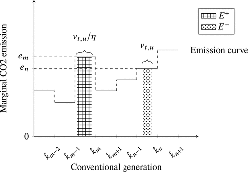
Hence, the transaction is -rate emission controlled if and only if , which is exactly Condition (22). When the storage transaction shifts market-clearing generators (and thus, prices), the marginal emission calculation becomes more complex. However, the proof of Theorem 3 establishes that the emission rates of such transactions cannot go beyond the maximal and minimal rates of the above-considered simple transactions (Condition (21)). Hence, Condition (22) remains sufficient in those cases as well.
Condition (22) formulates a tight requirement on storage-induced emissions at the transaction level in equilibrium while having a simple closed form and clear interpretation. Through profitable transactions, expensive conventional generation is replaced by cheaper alternatives. Condition (22) guarantees that this shift does not lead to emissions exceeding the acceptable threshold defined by . If , it is possible that when . However, for any —meaning that each profitable transaction must reduce emissions by at least —, we must have whenever . In this case, the interpretation is clear: to prevent storage agents from increasing pollution as CO2-intensive generators must be more expensive than cleaner ones. However, this is often not true in practice; for example, coal generation can be cheaper than gas in the absence of sufficiently high carbon pricing.
Furthermore, the theorem shows that simply aligning the merit-order curve with marginal emissions is not enough to ensure emission neutrality of storage; the inefficiency of storage must also be considered. The round-trip efficiency of storage () affects Condition (22) in two opposing ways. Higher efficiency expands the range of profitable transactions, making the condition more stringent as it applies to a broader set of trades. At the same time, increasing weakens the inequality in (22).
Finally, the results of Theorem 3 are robust regardless of residual demand, storage operations, or capacity. Instead, they depend only on the generator emission rates, merit-order curve, and storage inefficiency—factors that are relatively stable over time and known to the market operator. This allows the market operator to assess the conditions in advance (e.g., daily), evaluating the potential emission impact of a storage agent.
Note that the theoretical lower and upper bounds on the marginal emission rates per transaction in (21) are also bounds on the overall marginal emission rates of the storage by Lemma 2. Hence, using these bounds, one can evaluate the maximal potential of storage to reduce or increase pollution. Similarly, although Condition (22) is necessary and sufficient for -rate control at the transaction level, it also guarantees -rate control for the overall storage operation as shown in the corollary below (see Online Appendix EC.1.8 for the proof).
(
The analysis in this section and interval (21) provide a foundational framework for assessing the potential environmental impact of various storage agents differing by their round-trip efficiency (some examples are considered in Section 5). Moreover, Condition (22) can be utilized as a basis for developing policies aimed at mitigating storage marginal CO2 emission, which we will further explore in the next section.
4. Formulating a Carbon Levy to Mitigate Storage-Induced Emission
An effective approach to controlling storage marginal CO2 emissions is through a linear carbon levy. In our model, the levy represents a payment per unit of CO2 emitted. A fossil-based generator j with marginal emissions incurs a cost of for its output at time t, effectively shifting its marginal cost from to . This policy tool is already in use—for example, in carbon emission trading schemes, like the EU ETS. Although such levies apply only to emitting generators (not storage agents), we show that they can still indirectly and effectively reduce unintended storage-induced emissions. In this section, we formulate the carbon levy needed to satisfy Condition (22) from Theorem 3.
Carbon levies mitigate unintended storage-induced emissions by raising the marginal costs of fossil-fuel generators, thereby reshaping the merit-order curve and potentially satisfying Condition (22). To examine this effect more precisely, we first analyze the storage agent’s profitability under a carbon levy. Because the levy influences electricity prices, it shifts storage profits by redistributing gains from higher-emission transactions to those with lower emissions as shown in the following lemma (see Online Appendix EC.1.9 for the proof).
(
if , the profit of transaction decreases in ;
if , the profit of transaction does not change with ; and
if the profit of transaction increases in .
Lemma 3 shows that a positive carbon levy increases profits for transactions that potentially reduce emissions (i.e., when ) and reduces profits for those that may cause excessive emissions (i.e., when ), thereby discouraging the latter. Specifically, according to Lemma 3, any transaction violating Condition (22) from Theorem 3 becomes less profitable under a carbon levy, provided . As a result, a sufficiently high levy eliminates incentives for such transactions. When , however, the analysis becomes more nuanced as addressed in the next proposition (see Online Appendix EC.1.10 for the proof).
(
In the case of , (23) remains valid for only if for all .
Proposition 1 defines the minimum sufficient carbon levy. Any smaller levy would fail to satisfy the -rate emission control condition for some demand and RES realizations. Notably, Condition (23) is demand agnostic, ensuring that a levy above this threshold is robust to all possible demand and RES outcomes.
A carbon levy can ensure that each storage transaction does not exceed a nonnegative rate of marginal emissions (i.e., ). However, enforcing a negative marginal emission rate () per transaction through a carbon levy is generally infeasible. As shown in Lemma 3(c), the profitability of transactions with negative emission rates actually increases under a linear carbon levy. Because these transactions are already nonpolluting, the levy cannot further reduce their emissions. Achieving emission rates below a given negative threshold would require alternative instruments, such as levies applied directly to storage transactions to discourage specific behaviors. We leave the development of such mechanisms for future research.
A sufficiently high carbon levy eliminates all storage transactions that exceed a given nonnegative emission threshold. Thus, the theoretical upper bound from interval (21) on the marginal transaction-wise and overall emission rates of a storage agent (if positive) decreases with the levy. However, somewhat counterintuitively, this does not guarantee that the observed marginal emission rates for a given demand, RES, and storage volume scenario would decrease. The levy shifts the merit-order curve and changes the feasible set of transactions within a given scenario. For example, if all observed transactions initially have negative emission rates, a higher levy may make additional less clean (but still nonpolluting) transactions viable by Lemma 3(c), increasing the observed emission rates. Alternatively, when the levy does not eliminate all polluting transactions, a rise in the levy could make new polluting transactions feasible within the observed scenario because of the change in the merit order. In the next section, we demonstrate that such effects can occur in practice. This highlights a possible misalignment between policy goals; although a higher carbon levy cannot increase the total system CO2 emissions, it may paradoxically increase the emissions associated with storage.
We conclude with a corollary on the properties of the minimal carbon levy (see Online Appendix EC.1.11 for the proof).
(
The nonmonotonic relationship between the carbon levy and stems from opposing effects of on Condition (22). On one hand, higher expands the set of profitable transactions. On the other hand, as increases, fewer transactions satisfy , which can reduce the required levy.
5. Numerical Studies
In this section, we complement and support the above theoretical analysis with numerical studies using data from the Dutch electricity market. We work with the generation mix, marginal costs, and CO2 emissions data from the Dutch day-ahead electricity market during each day in two distinct years: 2019 and 2022. These years were deliberately selected because of their contrasting characteristics of demand, shares of renewable energy, and importantly, CO2 emission functions. We gathered the required market information from various sources as outlined in Table 2. We consider several types of storage: pumped hydro storage (PHS), compressed air energy storage, lithium-ion battery, hydrogen storage, and a hypothetical perfect energy storage system (perfect ESS) that has a perfect efficiency with no (dis-)charging-rate limitations and a negligible operational cost. Their respective parameters based on extensive research of open data sources are summarized in Table 3. The data sets and Python scripts used in this section are available on GitHub.
|
Table 2. Data Sources
| Variable | Data | Source |
|---|---|---|
| Fuel cost gas | Daily | Historic TTF market price |
| Fuel cost coal | Daily | Historic CIF ARA market price |
| EU ETS prices | Daily | Historic EU ETS price |
| Nuclear fuel cost | Mean 2019 and 2022 | “Economics of nuclear power” by World Nuclear Association (2025) |
| Operations and Management cost | Nuclear, coal, and gas plant | Lazard (2021) |
| Demand and renewable | Dutch day-ahead forecast 2019 and 2022 | “Transparency platform” by ENTSOE-E (2023) |
| Generators | Efficiency, CO2/GWh, capacity, min load, ramp up, ramp down | Kanellopoulos et al. (2019) |
Note. CIF ARA, cost, insurance and freight, Amsterdam Rotterdam, Antwerp; ENTSOE-E, E European Network of Transmission System Operators for Electricity; GWh, Gigawatt hour; TTF, title transfer facility.
|
Table 3. Storage Parameters
| Variable | PHS | CAES | Battery ion | Hydrogen | Perfect ESS |
|---|---|---|---|---|---|
| Round-trip efficiency | 0.76 | 0.795 | 0.9 | 0.375 | 1 |
| Maximum (dis-)charging rate (fraction of capacity/hour) | 0.12 | 0.19 | 0.57 | 1 | 1 |
| Round-trip Operation & Management cost (€/MWh) | 0.22 | 3.1 | 2.5 | 1 | 0.01 |
To find the optimal energy mix, we solve Problem (12). As inputs, we utilize the daily marginal cost of each generation facility, which encompasses fuel price, EU ETS price, and the facility’s efficiency. Our database includes 36 conventional generation facilities for 2019 and 38 conventional generation facilities for 2022, including parameters of their capacity, efficiency, and pollution rate. Using these data and the actual residual demand of the year, we solve Problem (12) for different storage technologies. In each case, we compute the profit of the storage agent using the market-clearing price extracted from the dual solution to Problem (12) according to Theorem 1.
5.1. Market Status Before Introducing Storage
Figure 2 shows the annual average daily merit-order curves for 2019 and 2022 based on fixed daily marginal costs (excluding renewables). Although over 36 generation facilities are included, we group them into four technology types, which are color coded in Figure 2 with darker shades indicating more polluting generators—nuclear, combined-cycle gas turbine (CCGT), gas peaker turbines, and coal. The top edges of the shaded areas in Figure 2 indicate the average yearly price for each unit of residual demand. The shaded composition at each capacity level in Figure 2 reflects the contribution of each technology to the average price. For instance, in 2019, a capacity of 7.5 GWh corresponds to an average price of 41.55€/GWh. At this capacity level, combined-cycle gas turbines account for 79% of this average price, whereas coal facilities contribute to the remainder—illustrating price variation between gas and coal over the year. Figure 2 also includes the yearly average marginal emission curve (right y axes). Residual demand is shown as box plots above each graph in Figure 2, indicating where market clearing occurs along the merit order. The box plots in Figure 2 display the interquartile range, with whiskers extending 1.5 times that range. Note that renewable generation is a part of residual demand, which explains its negative values. Although the residual demand varies hourly, the merit order is updated daily.
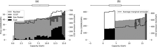
Notes. The “conflated” generation types are highlighted by different colors. The statistics of the residual demand are illustrated through the box plots on the top of the plots. (a) 2019. (b) 2022. CCGT, combined-cycle gas turbine; GWh, Gigawatt hour.
Figure 2 shows significant differences between 2019 and 2022, with prices in 2022 being notably higher because of increased fuel and EU ETS costs. Another difference is the stability of generating types’ positions in the merit order throughout the year. In 2022, gas-based assets were consistently more expensive than coal-based ones, whereas in 2019, coal was occasionally more expensive than gas. The marginal emission curve indicates that in 2022, a storage agent is more likely to replace low-polluting generators with high-polluting ones. If a storage agent displaces gas with coal, CO2 emissions increase. Yet, the residual demand is lower in 2022 because of higher renewable generation and reduced demand, leading to more instances of negative residual demand and greater opportunities for storage agents to help mitigate curtailment.
5.2. Market Status After Introducing Storage
By introducing a storage agent into the market based on the outcome of the system cost minimization Problem (12), we assess the overall storage marginal CO2 emissions for each year. Figure 3 shows the overall annual system emission changes because of storage participation (y axes) against storage capacity (as a percentage of the average daily demand; x axes) for each storage type. In 2019, all storage types reduce CO2 emissions, with reductions positively correlated to storage capacity and round-trip efficiency. In contrast, the impact in 2022 varies. Some storage types continue to reduce emissions, whereas others increase them. Emission changes in 2022 are not correlated with round-trip efficiency, unlike in 2019. These findings can be explained by combining the insights from Figure 2 and Section 3.2. In 2019, the marginal emission curve is mostly increasing within the interquantile range of residual demand, so the storage agent typically displaces more polluting generation with less polluting alternatives, reducing emissions. In contrast, 2022 shows a decreasing step in the emission curve within the interquantile range of residual demand coupled with more curtailment instances. Consequently, the storage agent both increases coal production and utilizes more renewable generation, leading to mixed effects on emissions.
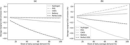
Notes. (a) 2019. (b) 2022.
The varying impacts of storage types highlight the importance of their parameters. Surprisingly, hydrogen, despite its low efficiency, achieves the greatest CO2 emission reduction in 2022. As shown in (19), storage with higher round-trip efficiency has more profit opportunities, leading to more transactions. The low efficiency of hydrogen storage makes many polluting transactions unprofitable. Hydrogen storage focuses on transactions with substantial spreads, such as charging from curtailed renewable energy or nuclear. This explains its superior emission reduction in 2022.
Although Figure 3 provides an overview of the overall storage marginal emissions per year, Figure 4 focuses on storage marginal emission rates at the transaction level. In the rest of this section, storage capacity is set to 10% of the daily average demand for each year. We decompose the optimal daily storage operation into profitable two-period transactions (as discussed in Online Appendix EC.1.5 via Algorithm 1) and calculate transaction-wise marginal emission rates (Definition 6). Figure 4 presents box plots of these rates for each year. Additionally, for each day, we compute the theoretical lower and upper bounds as stated in Theorem 3. In Figure 4, the highest daily theoretical upper bounds for the year are marked with ▲, and the lowest daily theoretical lower bounds for the year are marked with ▼. Figure 4 shows that the theoretical upper bound is not overly conservative as it is reached or nearly reached in all cases. Although there are more polluting transactions in 2022 than in 2019 (explaining the worse overall annual storage marginal emission in 2022 in Figure 3), the most polluting transactions have similar emission rates in both years. This suggests that although demand, generation costs, and emission patterns differ, the worst-case emissions remain similar. Also, there are more transactions reaching the theoretical lower bound (highest emission reduction) in 2022 in comparison with 2019.
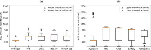
Notes. (a) 2019. (b) 2022.
Importantly, even small percentage changes in emissions are substantial; a 0.7% reduction in Dutch electricity emissions in 2019 corresponds to over 214,000 tons of CO2. As shown in Figure 4, the highest observed transaction-wise marginal emission rates in 2019 range from −376 tons CO2/GWh (hydrogen) to 638 tons CO2/GWh (pumped hydro storage). In 2022, this range shifts dramatically to the interval from 504 (perfect ESS) to 1,961 (hydrogen). The latter marginal emission is nearly three times as large as the one of the dirtiest generator. This observation indicates that low-efficiency storage can have substantially higher marginal emission than even the most polluting conventional generators, and it highlights the need to monitor transaction-level impacts to avoid excessive emissions.
5.3. The Impact of RES Generation Capacity
The relationship between RES and storage in market dynamics is complex. As noted by Peng et al. (2024), storage can either complement or substitute RES generation depending on market conditions. To assess this impact on storage emissions, we analyze how increased RES production—solar, wind, or both—affects storage transactions, focusing on battery storage. Figure 5(a) illustrates how storage’s CO2 impact evolves as RES scales up by x-fold (x axis). We consider three scenarios in Figure 5(a): scaling up total RES (“All RES”), scaling up only wind while keeping solar unchanged (“Wind”), and scaling up only solar while keeping wind unchanged (“Solar”). Both years follow similar trends, although at different scales because of residual demand differences. For instance, in 2022, lower initial residual demand and higher RES generation mean that a 10-fold RES increase in 2019 yields a similar residual demand to just a 5-fold increase in 2022.
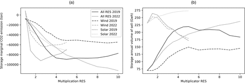
Notes. (a) Storage marginal CO2 emissions (b) Storage annual volume of sell.
Figure 5(a) shows that initially, greater RES penetration enhances storage’s ability to absorb green energy, displacing polluting sources and reducing overall emissions. However, this trend reverses as RES grows further, primarily because of its impact on price spreads, residual load, curtailments, and profitability. This nonmonotonic pattern is driven mainly by wind and not by solar. Scaling up wind power lowers residual demand (almost) uniformly, narrowing price spreads, reducing valley-filling potential, and increasing curtailment. In contrast, solar generation remains time concentrated, preserving valley-filling opportunities, as evidenced by Figure 6. Thus, as shown in Figure 5(b), storage transaction volume initially rises with wind expansion but later drops, whereas scaling solar consistently increases transactions. These observations align with the investment scenarios highlighted by Peng et al. (2024).
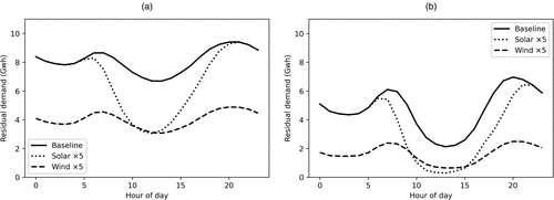
Notes. (a) 2019. (b) 2022.
To investigate this further, Figure 7 analyzes storage’s impact by categorizing transactions based on market-clearing generators. Each transaction is labeled , indicating charging from technology x and discharging to replace technology y. Figure 7 highlights solar’s and wind’s differing effects. We can see how complementing or substituting relationships between RES and storage impacts storage’s ability to reduce emissions. At moderate RES increases, storage complements RES by enabling “green” transactions—charging from otherwise curtailed RES and discharging to replace fossil fuels (i.e., ,, and ). However, as RES capacity grows further, these transactions decline in the wind scenario, a pattern absent in solar-only scenarios. This suggests that wind generation imposes greater constraints on storage’s ability to reduce curtailment and emissions by limiting opportunities of discharge. Thus, the “wind” scenario leads to higher res curtailment than the “solar” one.
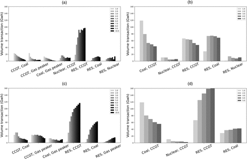
Notes. (a) Wind 2019. (b) Wind 2022. (c) Solar 2019. (d) Solar 2022.
Conversely, transactions where storage charges and discharges, whereas some fossil-fuel technologies are marginal generators (e.g., and ) decline in all scenarios, reflecting a substitutive effect between RES generation and storage, which leads to contrasting impacts. Namely, in 2019, this effect limits storage’s ability to reduce emissions by restricting transactions like . In 2022, it reduces storage’s potential to increase emissions by curbing transactions such as .
5.4. Carbon Levy
To mitigate unintended storage-induced emissions, we assess the carbon levy proposal from Section 4. Previously, generator marginal costs included EU ETS carbon prices. To isolate the impact of a storage-specific carbon levy, we remove the ETS component, setting a zero base for the theoretical levy. Figure 8 illustrates the levy’s effect on CO2 emissions across storage types. For each carbon levy rate , we solve Problem (12) using . Figure 8 presents (i) transaction-wise marginal emission-rate distributions (black box plots; comparable with Figure 4), (ii) yearly marginal emission rates (overall yearly storage emissions divided by yearly traded quantity), and (iii) worst-case theoretical upper and lower bounds per year.
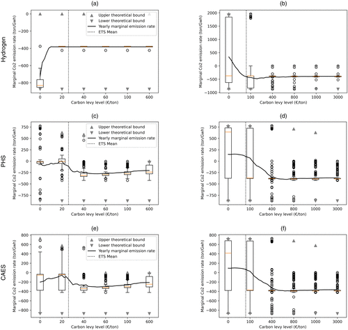
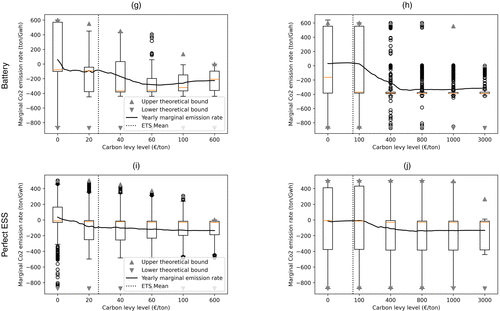
Notes. (a) Hydrogen 2019. (b) Hydrogen 2022. (c) PHS 2019. (d) PHS 2022. (e) CAES 2019. (f) CAES 2022. (g) Battery 2019. (h) Battery 2022. (i) Perfect ESS 2019. (j) Perfect ESS 2022.
Figure 8 shows that without a carbon levy, most storage transactions increase market emissions. As the levy grows, the distribution of storage transaction marginal emission shifts lower, and total market emissions decrease. However, the yearly marginal emission rates do not always decrease monotonically with the levy. For example, in 2019, hydrogen’s yearly marginal emission rate is lower without a levy than with a 20 €/ton levy. This counterintuitive outcome stems from two factors discussed in Section 4. First, as the levy rises, some nonpolluting transactions become profitable (Lemma 3), potentially leading to more storage transactions. However, these new transactions may be less effective in reducing emissions than those performed under a lower levy. Second, if generators are not ranked by marginal emissions in the merit order, a higher levy can shift their ranking, altering the set of feasible transactions for the same level of demand. Consequently, some high-emission transactions that were previously infeasible because of demand constraints may become viable for the storage agent. Paradoxically, in such cases, the storage agent might increase emissions under a higher carbon levy. However, this situation disappears with further increases in the carbon levy (after a certain levy level, all polluting transactions are not profitable by Proposition 1). Figure 8 also shows the average EU ETS prices for 2019 (26€/ton) and 2022 (81€/ton). Reducing storage-induced emissions requires a higher carbon levy in 2022 because of the merit-order shape discussed in Figure 2. In 2022, a levy exceeding the EU ETS price significantly lowers yearly marginal emission rates and reduces polluting transactions. In contrast, in 2019, raising the levy beyond the ETS level has minimal impact on yearly marginal emissions and transaction-level distributions.
Next, we evaluate the carbon levies proposed in Section 4. Figure 9 illustrates the yearly average minimal carbon levy defined in Proposition 1 against the maximal allowed transaction marginal emission rate in 2019 and 2022. The required levy is substantially higher in 2022 than in 2019 because of the emission curve shape discussed in Figure 2. When the maximum allowed transaction marginal emission rate tends to zero, the carbon levy tends to grow exponentially. For example, with a tolerance of 0 ton CO2/MWh for the perfect ESS, the carbon levy needs to be at least 380€/ton CO2 in 2019 and 3,902€/ton CO2 in 2022. For hydrogen, no levy is needed in 2019 because no polluting transactions exist, whereas in 2022, a flat levy of 120€/ton applies (just above the EU ETS price line). Although high in some cases, these levies will not necessarily hamper the total social welfare if the revenues from it are efficiently redistributed to society. Figure 9 also highlights the nonmonotonic relationship between round-trip efficiency and carbon levies as stated in Corollary 3. For example, for very small , the perfect ESS requires the highest carbon levy, whereas for high values, it requires the smallest one.
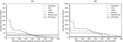
Notes. (a) 2019. (b) 2022.
Finally, we compare the theoretically sufficient carbon levy from Proposition 1 with the minimum required empirical levy. To obtain the latter, for each day, we conduct a line search to identify the lowest levy that achieves a given target for the observed demand. We then compute the ratio of the minimal required empirical levy to the theoretical levy. A value of indicates that the theoretical levy is tight for that day, whereas suggests that a lower levy suffices. Table 4 reports the highest of the year for three targets (, 100, 500 tons CO2/GWh). In most cases, the theoretical levy is tight on at least one day per year. However, for higher targets in 2022, throughout the year, indicating that lower levies are consistently sufficient.
|
Table 4. Maximum Ratio over the Year
| Year/Target | Hydrogen | PHS | CAES | Battery | Perfect ESS |
|---|---|---|---|---|---|
| (tons CO2/GWh) | |||||
| 2019 | No levy needed | 1 | 1 | 1 | 1 |
| 2022 | 0.54 | 1 | 0.1 | 1 | 1 |
| (tons CO2/GWh) | |||||
| 2019 | No levy needed | 1 | 1 | 1 | 1 |
| 2022 | 0.54 | 0.51 | 0.5 | 0.44 | 0.48 |
| (tons CO2/GWh) | |||||
| 2019 | No levy needed | 1 | 1 | 0.67 | 1 |
| 2022 | 1 | 0.51 | 0.53 | 0.87 | 1 |
Table 5 reports the 90th percentile of . For instance, with a target , the value for batteries is 0.81—indicating that on at least 10% of days in 2022, the empirical levy was at least 81% of the theoretical value. The 90th percentile values are substantially lower than the maximum values, highlighting that although the theoretical levy is conservative and ensures worst-case coverage, lower levies are sufficient on most days.
|
Table 5. Ninetieth Percentile of Ratio over the Year
| Year/Target | Hydrogen | PHS | CAES | Battery | Perfect ESS |
|---|---|---|---|---|---|
| (tons CO2/GWh) | |||||
| 2019 | No levy needed | 0.53 | 0 | 0.54 | 0.31 |
| 2022 | 0.34 | 0.22 | 0.08 | 0.28 | 0.65 |
| (tons CO2/GWh) | |||||
| 2019 | No levy needed | 0.53 | 0 | 0.54 | 0.72 |
| 2022 | 0.34 | 0.46 | 0.45 | 0.41 | 0.41 |
| (tons CO2/GWh) | |||||
| 2019 | No levy needed | 0.65 | 0 | 0.19 | 0 |
| 2022 | 1 | 0.46 | 0.47 | 0.81 | 0 |
5.5. Profit of Storage Agents
Figure 10 illustrates the percentage change in annual total profit for each storage agent under varying carbon levy levels relative to the no-levy baseline. Two distinct regions emerge. In the low-levy region, profits show little to no consistent increase and may even decline slightly. As indicated by Lemma 3, this pattern arises because some previously profitable but polluting transactions become unviable, whereas the gains from cleaner transactions are not yet sufficient to compensate for the loss. Once the levy surpasses a critical threshold, the system enters the second region, where profits grow steadily and monotonically with increasing levy. This shift aligns with our theoretical results. Proposition 1 shows that above this threshold, only nonpolluting transactions remain profitable, whereas Lemma 3 confirms that profits per transaction increase as the levy rises. Together, these results explain the rapid and sustained profit growth observed for all storage types once the threshold is crossed. This threshold is significantly higher in 2022 than in 2019 as demonstrated in Figures 8 and 9: around €10/ton CO2 in 2019 and approximately €150/ton CO2 in 2022. Notably, in 2019, the threshold lies below the prevailing ETS price, whereas in 2022, it exceeds it, suggesting that higher EU ETS prices could enhance both the profitability and environmental performance of storage operations.
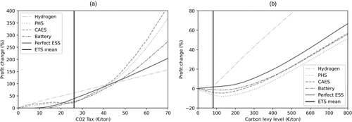
Notes. (a) 2019. (b) 2022.
5.6. The Impact of the Generator’s Technical Constraints
For analytical simplicity, we initially disregarded some of the generators’ technical constraints, specifically start-up costs, ramping limits, and minimum load. A theoretical analysis of these constraints is provided in Online Appendix EC.2. In summary, our core theoretical results about the equivalence of joint and individual optimization (Theorem 1) as well as the decomposition of the total emission into transaction-wise emissions (Section 3.2 up to Theorem 3) remain valid under these constraints. However, each constraint type introduces its own complications in estimating upper and lower bounds on the marginal transaction-wise emission rates as undertaken in Theorem 3. Below, we numerically assess their impacts by introducing each constraint individually and comparing the results with the unconstrained case. Minimum-load and ramping data are sourced from the European Network of Transmission System Operators for Electricity (ENTSOE-E 2023), whereas start-up costs are estimated from the International Energy Agency (2014). We evaluate how these constraints affect emissions and the role of storage in mitigating them.
5.6.1. Start-up Costs.
Including the start-up cost constraint has no impact on total emissions or the contribution of storage to them. Given the minimal changes, we omit the corresponding figures for brevity. This indicates that overall emissions and storage-driven CO2 effects remain effectively unchanged. In theory, the transaction types analyzed in our simplified model remain valid under start-up costs; yet, start-up costs could introduce some new transaction types whose marginal emission rates could potentially fall outside the theoretical bound established in Theorem 3. Nevertheless, we do not observe such deviations in the data.
5.6.2. Minimum Load.
The minimum-load constraint has only a limited effect on our results; therefore, the corresponding figures are omitted for brevity. Theoretically, the impact of the minimum-load constraint mirrors that of start-up costs; the transactions derived in our simplified model remain valid, although additional types of equilibria or dispatch patterns may emerge. Hence, the largest and lowest marginal emission rates may fall outside the bounds from Theorem 3; see Online Appendix EC.2 for more details. Without storage, minimum load increases emissions by only 0.02% in 2019 and 0.003% in 2022. The impact is greater in 2019 as coal replaces CCGT, whereas in 2022, coal is already heavily dispatched, making the constraint less relevant. Storage behaves similarly to the unconstrained case, with slightly amplified effects. Finally, over 92% of 2019 transaction volumes and 94.2% of 2022 transaction volumes remain within the theoretical interval.
5.6.3. Ramping Constraint.
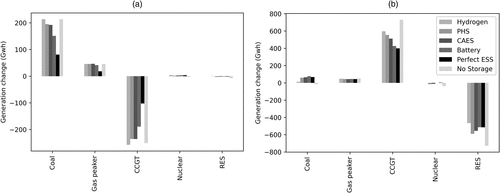
Unlike start-up costs and minimum load, ramping constraints have a more pronounced effect on the equilibrium and emissions. Figure 11, analogous to Figure 3 but with ramp-rate limits, illustrates this impact. Without storage, ramping constraints increase emissions by 0.4% in 2019 and 1.2% in 2022. Storage reduces this increase by providing flexible support to generator inflexibility. Comparing Figure 11 with Figure 3, we find that in 2019, all storage types achieve greater emission reductions, maintaining the same ranking as in the unconstrained case. In 2022, all storage types now reduce emissions unlike before, although their ranking still does not align with round-trip efficiency.
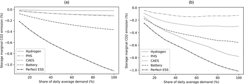
Notes. (a) 2019. (b) 2022.
To investigate further, Figure 12 shows the marginal impact of ramping constraint on the generation of each technology. Coal output increases in both years, primarily displacing flexible assets—CCGT in 2019 and RES in 2022. This indicates that ramping constraints force inflexible generators to produce more across adjacent periods, displacing cleaner technologies and contributing to higher CO2 emissions. Further analysis of Figure 12 reveals that storage reduces emissions through different mechanisms. In 2019, it limits coal’s rise and maintains CCGT output, whereas in 2022, it prevents some RES curtailment. However, the 2022 benefit is offset by a larger coal increase relative to CCGT, explaining the nonmonotonic emission effects. Overall, under ramping constraints, storage has a stronger influence on both emissions and the generation mix, with its impact more pronounced under favorable conditions as seen in 2019.
Notes. (a) 2019. (b) 2022.
It is also important to assess how ramping constraint affects the theoretical upper and lower bounds on the transaction pollution rate established in Theorem 3. Because this constraint is not considered in the theorem, we examine the extent of bound violations when ramp rates are imposed. Table 6 summarizes the results; each column in Table 6 shows the degree of violation (as a percentage of the theoretical bounds), and each row in Table 6 corresponds to a technology with 10% of daily average demand capacity. Each cell indicates the percentage of transactions for that technology (in volume) experiencing the specified violation. As shown in Table 6, the theoretical upper bound is largely respected; most technologies see only minor violations, and violations above 1% are rare. This suggests that ramping constraints might have only minimal impact on the worst-case pollution rate. A larger share of transactions violates the lower bound, suggesting that ramping constraints result in more pollution-reducing transactions than would occur without considering the constraint.
|
Table 6. Impact of the Ramping-Rate Constraint on Violating the Theoretical Upper and Lower Bounds
| Technology/violation of bound, % | 2019 | 2022 | ||||
|---|---|---|---|---|---|---|
| 0% | 0% | |||||
| Upper-bound violations, % of total volume of all transactions | ||||||
| Hydrogen | 98.4 | 98.4 | 1.6 | 75.7 | 85.7 | 14.3 |
| PHS | 95.6 | 95.6 | 4.4 | 84.2 | 97.8 | 2.2 |
| CAES | 96.6 | 96.6 | 3.4 | 81.9 | 97.8 | 2.2 |
| Battery | 98 | 98.9 | 1.1 | 72.2 | 95.2 | 4.8 |
| Perfect ESS | 92.4 | 97.9 | 2.1 | 79.6 | 95.2 | 4.6 |
| Lower-bound violations, % of total volume of all transactions | ||||||
| Hydrogen | 98.9 | 100 | — | 71.1 | 84.3 | 15.7 |
| PHS | 90.2 | 98.5 | 1.5 | 81 | 92.8 | 7.2 |
| CAES | 91 | 99.3 | 0.7 | 78.9 | 91.2 | 8.8 |
| Battery | 88.4 | 99.4 | 0.6 | 77.2 | 88.6 | 11.4 |
| Perfect ESS | 94 | 99.7 | 0.3 | 83.5 | 93 | 7 |
In summary, among the three constraints studied, ramping constraints appear the most consequential. This is consistent with our theoretical analysis in Online Appendix EC.2; for this type of constraint, not only the transaction types would change in comparison with our simplified model but also, the market prices, which complicates detecting profitable transactions. Nonetheless, even in the case of ramping constraints, the core conclusions of this study regarding storage’s role in emissions remain unaffected. In fact, although this study focuses on the worst-case indirect emissions of storage, our experimental results show that storage could be slightly more beneficial in reducing emissions under ramping constraints, reinforcing its value as a green asset.
6. Conclusions
As the energy transition shifts from fossil fuels to intermittent sources, like wind and solar, revenue and supply-demand uncertainties rise. To manage this intermittency, flexible resources—particularly large-scale storage—are expanding alongside renewable penetration. This study examines whether integrating such large-scale storage is carbon neutral. Although storage operations themselves are emission free, their influence on the dispatch of other generators can indirectly affect overall system emissions. From a sustainability standpoint, these often-overlooked scope 2 impacts may be significant.
We analyzed the impact of storage activities on electricity markets at the highest resolution (transaction level), identifying when and why storage can increase emissions. We formulated tight lower and upper bounds on marginal emission rates of storage depending on the generation mix of the market and storage type. The upper bound defines conditions under which storage integration aligns with emission targets. Building on these conditions, we derived a minimum carbon levy sufficient to ensure that a storage agent does not increase emissions beyond target limits. To support our theoretical findings, we conducted detailed numerical studies using real-world data from two distinct years in the Dutch electricity market. Our combined analytical and numerical results offer several novel insights. We also show how these results are impacted by technical constraints of conventional generators, such as start-up costs, minimum load, and ramping. Finally, we analyze how RES and storage interplay in terms of emission.
The findings of this paper can inform policymakers on how to integrate storage into electricity markets without compromising decarbonization goals. For example, we showed that there is no monotonic relationship between storage round-trip efficiency and its worst-case emission impact; although higher efficiency reduces reliance on “dirty” energy, it also allows access to a wider set of potentially polluting transactions. A carbon levy can effectively limit unintended emissions from storage. However, for the levy to be effective, it needs to render the marginal emission cost curve steep enough to counteract storage inefficiencies. This means that higher carbon prices may be required for storage than those typically seen in cap-and-trade schemes. The required levy increases as emission targets become more stringent, but interestingly, a higher levy does not always translate to lower observed emissions. We also found that more efficient storage may require a higher carbon levy to meet the same emission target. Lastly, we showed that indirect emissions of storage agents are also influenced by whether solar or wind dominates the renewable mix.
This study provides one of the most detailed analyses of storage-induced emissions, capturing essential market and storage dynamics. Although certain real-world factors, such as network congestion or multimarket participation, are excluded from our examination, this simplification facilitates the derivation of clear and generalizable insights. Yet, these extensions could be promising avenues for future studies. Our framework is designed to be robust against uncertainties in demand, renewable generation, and storage agent behavior, including variations in size and market strategy. The framework also allows for the robust incorporation of interval uncertainty in marginal costs and emission rates. This robustness introduces, however, a degree of conservatism, which may be relaxed through probabilistic approaches better suited to regulators that wish to target more flexible standards. Overall, our work brings clarity to the often-overlooked carbon implications of storage—an increasingly important consideration in designing sustainable, low-carbon power systems.
References
- (2019) The role of energy storage in deep decarbonization of electricity production. Nature Comm. 10(1):3413.Crossref, Google Scholar
- (2018) Tradeoffs between revenue and emissions in energy storage operation. Energy 143:1–11. Crossref, Google Scholar
- (2021) An experimental study of monthly electricity demand (in) elasticity. Energy J. 42(2):205–222.Crossref, Google Scholar
- (2013) The private and social economics of bulk electricity storage. J. Environ. Econom. Management 66(3):404–423.Crossref, Google Scholar
- (2019) Why 100% renewable energy is not enough. Joule 3(6):1389–1393.Crossref, Google Scholar
- (2016) The value of energy storage in decarbonizing the electricity sector. Appl. Energy 175:368–379.Crossref, Google Scholar
ENTSOE-E (2023) Transparency platform. Retrieved January 27, https://transparency.entsoe.eu/.Google Scholar- (2017) Emissions and economics of behind-the-meter electricity storage. Environ. Sci. Tech. 51(3):1094–1101.Crossref, Google Scholar
- (2021) The effect of price-based demand response on carbon emissions in European electricity markets: The importance of adequate carbon prices. Appl. Energy 295:117040.Crossref, Google Scholar
- (2019) How much wind and solar are needed to realize emissions benefits from storage? Energy Systems 10(2):437–459.Crossref, Google Scholar
- (2021) How does new energy storage affect the operation and revenue of existing generation? Appl. Energy 285:116383.Crossref, Google Scholar
- (2019) JRC open power plants database (JRC-PPDB-OPEN), European Commission, Joint Research Center (JRC). Retrieved September 28, 2022, http://data.europa.eu/89h/9810feeb-f062-49cd-8e76-8d8cfd488a05.Google Scholar
- (2015) Bulk energy storage increases United States electricity system emissions. Environ. Sci. Tech. 49(5):3203–3210.Crossref, Google Scholar
IEA (2014) The power of transformation. IEA, Paris, https://www.iea.org/reports/the-power-of-transformation, Licence: CC BY 4.0.Google ScholarIEA (2024) Batteries and secure energy transitions. IEA, Paris, https://www.iea.org/reports/batteries-and-secure-energy-transitions, Licence: CC BY 4.0.Google ScholarLazard (2021) Lazard’s levelized cost of energy analysis—Version 15. Technical report, Lazard, London.Google Scholar- (2023) The value of coordination in multimarket bidding of grid energy storage. Oper. Res. 71(1):1–22.Link, Google Scholar
- (2020) Profitable emissions-reducing energy storage. IEEE Trans. Power Systems 35(2):1509–1519.Crossref, Google Scholar
- (2024) Renewable, flexible, and storage capacities: Friends or foes? Manufacturing Service Oper. Management 26(5):1730–1749.Link, Google Scholar
- (2023) The role of electricity market design for energy storage in cost-efficient decarbonization. Joule 7(6):1227–1240.Crossref, Google Scholar
- (2024) On the means, costs, and system-level impacts of 24/7 carbon-free energy procurement. Energy Strategy Rev. 54:101488.Crossref, Google Scholar
- (2016) Comparative assessment of models and methods to calculate grid electricity emissions. Environ. Sci. Tech. 50(17):8937–8953.Crossref, Google Scholar
- (2016) Economic assessment of a price-maker energy storage facility in the Alberta electricity market. Energy 111:537–547.Crossref, Google Scholar
- (2024) Electricity pricing rules with residential solar-plus-storage: Economic and environmental impacts. Preprint, submitted July 19, http://dx.doi.org/10.2139/ssrn.4899728.Google Scholar
The World Bank (2025) State and trends of carbon pricing dashboard. Retrieved November 2025, https://carbonpricingdashboard.worldbank.org/.Google Scholar- (2022) Electricity storage and market power. Energy Policy 164:112872.Crossref, Google Scholar
World Nuclear Association (2025) Economics of nuclear power. Accessed October 18, 2022, https://world-nuclear.org/.Google Scholar- (2013) Curtailing intermittent generation in electrical systems. Manufacturing Service Oper. Management 15(4):578–595.Link, Google Scholar
- (2023) On the distributed energy storage investment and operations. Manufacturing Service Oper. Management 25(6):2277–2297.Abstract, Google Scholar
- (2023) The social cost of carbon when we wish for full-path robustness. Management Sci. 69(12):7585–7606.Link, Google Scholar
- (2016) Electricity trading and negative prices: Storage vs. disposal. Management Sci. 62(3):880–898.Link, Google Scholar