


Conformal Inverse Optimization for Adherence-Aware Prescriptive Analytics
Abstract
Inverse optimization is increasingly used to estimate unknown parameters in an optimization model based on decision data. However, when such point estimates are used to prescribe downstream decisions, the resulting decisions may be of low quality and misaligned with human intuition and, thus, less likely to be adopted. To tackle this challenge, we propose a prescriptive analytics pipeline that learns an uncertainty set for the unknown parameters and then solves a robust optimization model to prescribe new decisions. We show that the suggested decisions can achieve bounded optimality gaps as evaluated using both the ground truth parameters and human perceptions. Our method demonstrates strong empirical performance compared with the standard inverse optimization pipeline. Finally, we perform a simulated case study in which we apply this new pipeline to provide delivery route recommendations in Toronto, Canada. In this case study, our approach achieves a significantly higher delivery path adherence rate than current industry practices without compromising service quality. Moreover, our method provides a better trade-off between absolute and perceived decision quality under realistic scenarios, including cases with model misspecification and data scarcity.
Funding: E. Delage was partially supported by the Canadian Natural Sciences and Engineering Research Council [Grant RGPIN-2022-05261] and by the Canada Research Chair program [Grant 950-230057]. T. C. Y. Chan and B. Lin were partially supported by the Natural Sciences and Engineering Research Council of Canada Alliance [Grant 561212-20]. B. Lin was also supported by the National University of Singapore [Grant A-0010602-00-00].
Supplemental Material: All supplemental materials, including the code, data, and files required to reproduce the results, are available at https://doi.org/10.1287/opre.2024.1376.
1. Introduction
Inverse optimization (IO) is increasingly used to estimate unknown parameters in optimization models from decision data, after which the calibrated models can be used to prescribe prospective decisions in new contexts. Such estimate-then-optimize pipelines are applied across a range of domains, including vehicle routing (Rönnqvist et al. 2017, Zattoni Scroccaro et al. 2024a), last-mile delivery (Wang et al. 2025), transportation network design (Liu et al. 2024), radiation therapy treatment planning (Chan et al. 2014, Babier et al. 2020), portfolio optimization (Dong and Zeng 2021), and airline crew scheduling (Wei and Vaze 2018).
Despite these successes, prescriptive IO pipelines that rely on a point estimate may not always be effective. First, in many applications, decision data are generated by heterogeneous decision makers, and the parameters to be estimated represent their preferences or tacit knowledge (see, e.g., Merchán et al. 2022) that may vary widely across individuals (Lobo and Yao 2025). Consequently, a single point estimate may have limited value because of the lack of consensus among individuals. Second, the specified optimization model may not perfectly capture the human decision-making process, further limiting the generalization power of such estimates. Finally, even when decision makers are homogeneous and the model is well-specified, many IO approaches do not provide statistically consistent estimates and can be sensitive to data noise (Shahmoradi and Lee 2022). Whereas consistent IO estimators exist for strictly convex problems (Aswani et al. 2019), solving the resulting IO models is computationally challenging. In many practical settings, applying computationally tractable but inconsistent IO estimators to noisy data sets is the only realistic option. Nontrivial estimation errors may, therefore, arise no matter how large the data set is, and these errors can be significantly amplified in the downstream decision prescription process (Elmachtoub and Grigas 2022), leading to an unstable pipeline.
In this paper, we address this issue by robustifying the downstream optimization model to hedge against IO estimation errors. Whereas different forms of this strategy are shown to be effective in the broader data-driven optimization literature (Sadana et al. 2025), applying it in IO settings is challenging as the parameters of interest are, by definition, unobservable. For instance, they may represent latent weights in a multiobjective optimization model (Chan et al. 2014, Zattoni Scroccaro et al. 2024a, Wang et al. 2025), and these are intrinsically difficult to observe. As a result, uncertainty set construction methods from the robust optimization literature (e.g., Shang et al. 2017, Chenreddy et al. 2022, Goerigk and Kurtz 2023), which typically rely on such observations, are not applicable. This limitation calls for new methods that construct uncertainty sets from decision data and integrate them into the downstream optimization process.
In response, we propose a prescriptive analytics pipeline that requires only decision data and is flexible enough to incorporate observed parameters when they are available. First, we develop an IO method that returns not only a point estimate but also an uncertainty set calibrated around that estimate. This method can be used to estimate unknown parameters in an objective function that is linear in those parameters. Having an uncertainty set is particularly important in this setting as such problems typically do not satisfy the strict convexity conditions required for consistent IO estimators. Next, the uncertainty set is incorporated into a robust optimization model for decision prescription. When available, observed parameters can be leveraged to regularize the robust optimization model. Finally, we develop algorithms to accelerate both the uncertainty set calibration and the solution of the robust optimization model. Whereas this IO pipeline is general, it is motivated by practical challenges in human–AI interaction, in which the quality of the prescribed decisions can be defined both objectively and subjectively, creating additional nuances in our analysis.
1.1. Practical Motivation: Algorithm Adherence
AI techniques demonstrate strong performance across many tasks, yet humans may still be reluctant to adopt these techniques, a phenomenon known as algorithm aversion (Burton et al. 2020). In many operational settings, such deviations can be costly. For instance, Alibaba developed an algorithm to optimize delivery box packing. However, workers in their warehouse did not conform to algorithm-suggested packing plans for 5.8% of the packages, and these packages experienced a 48.3% increase in processing time compared with the recommended plan (Sun et al. 2022). Similarly, when an automobile parts retailer used a data-driven tool to identify low-performing stock-keeping units for removal from local stores, recommendations were overridden more than 50% of the time by local merchants, leading to an estimated 5.8% reduction in profitability (Kesavan and Kushwaha 2020). Deviations may also have other negative consequences besides degraded solution quality. For example, a rideshare driver’s deviation from the recommended path may raise rider safety concerns (Global Times 2021) and affect other platform functions that rely on route predictions, such as arrival time estimation (Hu et al. 2022).
Empirical research identifies the alignment between algorithmic recommendations and human perception as a key factor influencing algorithm adoption (Chen et al. 2023, Liu et al. 2023, Bastani et al. 2025). The essence of the issue is that an algorithm may present a decision that is optimal according to objective criteria but is perceived as suboptimal under subjective human judgment. As a result, human decision makers may reject the recommendation and implement an alternative decision even when they would have accepted a slightly suboptimal recommendation that better aligns with their judgment. For the successful deployment of data-driven decision support tools, it is critical to derive decisions that are not only high quality according to objective criteria but also perceived as high quality by human decision makers.
Indeed, there is increasing attention from both academia (Martínez-de Albéniz and Krigul 2025, Wang et al. 2026) and industry (Merchán et al. 2022) calling for algorithmic designs that better align with human perception. In such contexts, IO offers a methodology for inferring unobservable human perceptions from observed decisions, aiming to derive recommendations that are high quality both objectively and subjectively. Because such decision data sets are often crowd-sourced from heterogeneous decision makers, it is crucial to design an IO pipeline that captures this variability and is robust to estimation errors. These considerations motivate the IO pipeline and theoretical analysis developed in this paper.
1.2. Contributions
A new framework: We propose a prescriptive analytics pipeline to generate decisions that are of high quality and aligned with human intuition. Our pipeline integrates (i) conformal IO, a novel approach to constructing uncertainty sets based on decision data and (ii) a robust optimization model for decision recommendation. Item (i) may be of independent interest to the data-driven robust optimization community as it presents a new way to construct uncertainty sets without observations of the unknown parameters. Whereas the resulting worst case value problem in the robust model is nonconvex, we introduce a data-driven method to approximate it for the case in which the objective components and unknown parameters are nonnegative with provable solution quality guarantees. This method can be generalized to solve other norm-constrained robust optimization problems.
Theoretical guarantees: We prove that the probability of the learned uncertainty set containing parameters that make future observed decisions optimal always exceeds a specified threshold (conservatively valid), and this probability converges to the threshold as the sample size goes to infinity (asymptotically exact). This coverage guarantee leads to provable bounds on the optimality gap of the decisions from conformal IO as evaluated using both the ground truth parameters and the decision maker’s perceived parameters.
Performance: Through extensive numerical experiments, we (i) verify the effectiveness of conformal IO in constructing an uncertainty set that achieves the out-of-sample coverage desired by the model user, (ii) demonstrate better performance of our conformal IO pipeline compared with the standard IO pipeline in terms of ground truth and perceived solution quality, and (iii) show that our data-driven approximation to the nonconvex robust optimization model significantly improves the computational efficiency of our pipeline and maintains high decision quality.
Case study: Using a mix of real and simulated data, we perform a case study in which we apply the proposed approach to provide route recommendations for food delivery couriers in Toronto, Canada, leading to a rich set of managerial insights. In this case study, we estimate that, compared with the current industry practice that recommends the shortest delivery route, our approach may improve the path adherence rate by 8.75–62.5 percentage points, incurring comparable delivery time. When couriers have a low tolerance for suboptimal (with respect to their own perceptions) path recommendations, we can achieve shorter average delivery time than recommending the shortest path (with respect to ground truth parameters) because we prevent couriers from deviating and choosing a perceived optimal path that turns out to take more time. This finding underscores the opportunity for a win–win: improved recommendation adherence and improved service quality. When we benchmark against the standard IO pipeline, our pipeline offers a better trade-off between absolute and perceived decision quality. It also demonstrates more robust performance when the optimization model is misspecified. In a third experiment, we compare our model against a personalization strategy that maintains one model for each courier, varying the number of data points observed for each courier. Our method incurs lower computational overhead and demonstrates stronger performance in data-poor regimes with comparable performance in data-rich regimes. This finding highlights the value of our approach when the platform enters a new market or is onboarding new couriers, for example.
All proofs are in the Online Electronic Companion. The data and code used to implement our algorithm are available at https://github.com/lin-bo/ConformalInverseOptimization.
2. Literature Review
Our paper is related to a broad range of literature, including inverse optimization, estimate then optimize, data-driven robust optimization, and human–AI interaction.
IO aims to impute unknown parameters in an optimization model based on decision data in both off-line (Ahuja and Orlin 2001, Bertsimas et al. 2015, Chan and Kaw 2020, Birge et al. 2022b) and online settings (Dong et al. 2018, Bärmann et al. 2018, Besbes et al. 2025) in which data are observed sequentially. Early IO papers focus on deterministic settings in which the observed decisions are assumed to be optimal to the specified optimization model. Recent papers focus on stochastic settings in which the observed decisions are noisy. When the decision data are subject to execution errors, Aswani et al. (2018) propose an IO model that minimizes the predictability loss, leading to a statistically consistent estimator for strictly convex problems. When the decision data are subject to model misspecification, measurement error, and bounded rationality, Mohajerin Esfahani et al. (2018) propose a distributionally robust suboptimality loss and derive generalization bounds for the IO estimate. Chan et al. (2019) study similar suboptimality losses and demonstrate their tractability given noisy decision data. We refer readers to Chan et al. (2023a) for a comprehensive review. In this paper, we focus on another source of noise; our decision data are generated using possibly biased human perception of the ground truth parameters. Our IO pipeline utilizes the suboptimality loss of Mohajerin Esfahani et al. (2018) and Chan et al. (2019) as we focus on developing a computationally tractable pipeline that can be applied to both continuous and discrete optimization models. Moreover, we derive theoretical guarantees on absolute and perceived solution quality for our prescribed decisions, which has not been studied in the IO literature.
The above IO methods all return a point estimate of the target parameters, whereas our goal is to learn an uncertainty set. Recently, Birge et al. (2022a) and Yousefi (2023) present IO approaches for estimating a parameter distribution, which can also be used to construct an uncertainty set. The former approach relies on distributional assumptions regarding the unknown parameters, whereas the latter relies on an identifiability condition being satisfied. Both papers rely on posterior sampling algorithms to solve the IO problem, which is computationally demanding and cannot deal with more than a few parameters. In this paper, we do not impose any distributional assumptions regarding the unknown parameters, so the method by Birge et al. (2022a) is not applicable. Moreover, we focus on a class of problems whose objective function is linear in the unknown parameters, which violates the identifiability condition used by Yousefi (2023).
Our approach belongs to the family of estimate-then-optimize methods. Recent studies suggest that estimation errors may be amplified in the optimization step, leading to significant decision errors. This issue can be mitigated by training the estimation model with decision-aware losses (Wilder et al. 2019, Elmachtoub and Grigas 2022, Mandi et al. 2022) and robustifying the optimization model (Chan et al. 2023b, Sun et al. 2023). We are similar to the second stream, but differ by (i) using decision data instead of observations of the unknown parameters and (ii) focusing on both absolute and perceived solution quality, the latter of which has not been studied.
Uncertainty set construction for robust optimization has been extensively studied. Central to this problem are the tractability of the resulting robust model and the price of robustness. Early papers use prior knowledge about the parameter uncertainty to design sets that are polyhedral (Ben-Tal and Nemirovski 1999), ellipsoidal (Ben-Tal and Nemirovski 2000), cardinality-constrained (Bertsimas and Sim 2004), and norm-constrained (Bertsimas et al. 2004). Recently, data have become a critical ingredient in defining new uncertainty sets for distributionally robust optimization (Delage and Ye 2010, Mohajerin Esfahani et al. 2018, Gao and Kleywegt 2023) and calibrating the size of the uncertainty set (Bertsimas et al. 2018, Chenreddy et al. 2022). Closest to our work are Hong et al. (2021) and Sun et al. (2023), who use conformal prediction to calibrate uncertainty set sizes. Whereas conceptually similar, there is a key distinction: their methods require observations of the unknown parameters, which we assume are unavailable or unobservable. In contrast, we propose the first method for calibrating uncertainty sets using decision data alone, which are more readily observed in many applications. Moreover, whereas Hong et al. (2021) and Sun et al. (2023) aim to construct sets that cover future parameter realizations with a specified probability, our goal is to identify sets that contain parameters capable of rationalizing future decisions with a specified probability.
Our paper relates to human–AI interaction. Empirical studies identify factors that explain algorithm aversion, including poor performance (Yin et al. 2019) and the lack of human control (Dietvorst et al. 2018), human inputs (Kawaguchi 2021), or transparency (Kizilcec 2016). In response, researchers propose algorithms that are interpretable (Ciocan and Mišić 2022, Bastani et al. 2025) and adherence-aware (Grand-Clément and Pauphilet 2024), leading to improved human–AI collaboration. Our paper shares the same goal, but focuses on improving the alignment between algorithmic recommendation and human perception, which is identified as another major factor that affects algorithm adoption (Chen et al. 2023, Liu et al. 2023). Closest to our paper is Fu et al. (2023), who combine driver routing preferences learned using inverse reinforcement learning with the theoretical shortest path to prescribe last-mile delivery routes. In contrast, our method is not specific to last-mile delivery. Additionally, we characterize the concepts of actual and perceived optimality gaps and derive theoretical guarantees for our model’s performance.
3. Preliminaries
In this section, we present the problem setup (Section 3.1) and discuss the challenges associated with the standard IO pipeline (Sections 3.2 and 3.3). To address these challenges, we introduce a new IO pipeline that incorporates robustness into the decision recommendation process (Sections 3.4 and 3.5) and provide theoretical results that explain why adding robustness can be beneficial (Section 3.6).
3.1. Problem Setup
Consider N decision makers, each solving an optimization problem. The feasible region for decision maker is parameterized by some observed exogenous parameters , whereas the objective is parameterized by some unobserved parameters representing the decision maker’s perception. There also exist ground truth parameters that may be known or unknown and that correspond to an objective evaluation criterion. Let denote decision maker k’s decision made based on and . Given a data set , we are interested in designing a decision policy that recommends a decision for any future . We seek a policy such that the prescribed decision is of high quality with respect to both and a future .
(
(
3.1.1. Data-Generation Process.
Consider a forward optimization problem:
We focus on the case in which f is linear in . That is, the objective of can be written as
(
(
3.1.2. Evaluation Metrics.
We propose the following two metrics to evaluate .
The actual optimality gap (AOG) of a decision policy is defined as
The perceived optimality gap (POG) of a decision policy is defined as
AOG is an objective performance metric that measures the absolute solution quality, that is, with respect to . In contrast, POG is a subjective metric that measures the decision quality perceived by humans. Our goal is to design a decision policy that has low AOG and POG simultaneously, so the recommendations generated by are of high quality and likely to be implemented.
(
(
3.1.3. Assumptions and Definitions.
We introduce two mild assumptions on the data-generation process and define a constant that later appears in our bounds.
The data set is generated using , where are independent and identically distributed (i.i.d.) samples from for all .
There exists a constant such that .
Define to be a constant such that for any , , and , where .
Assumption 1 is standard in the data-driven optimization literature. Assumption 2 simply states that the distance between the expected value of the perceived parameters and the ground truth parameters is bounded. We know such a constant exists because the support of lies within the unit ball (recall Section 3.1.1). We expect to be moderate in many settings, such as in routing, in which drivers develop a good sense of travel times over repeated experience. Similar ideas motivate prediction markets, in which aggregated beliefs often outperform individual estimates and are close to the ground truth (see Chen and Zhao 2025 for a review). The constant in Definition 3 exists as is bounded because of the norm constraint.
3.2. Standard Inverse Optimization Pipeline
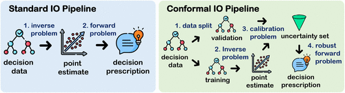
A natural approach to solving the learning task, referred to as the standard IO pipeline (visualized in Figure 1), is to first use IO to obtain a point estimate of the unknown parameters and then employ a policy to prescribe decisions for any , that is, solving with the estimated and .
Specifically, given , we can estimate the parameters by solving the following inverse optimization problem:
The suboptimality loss of is given by
Whereas this loss function does not produce statistically consistent estimates of the parameters (Aswani et al. 2018), it is the most commonly used because it is tractable. In fact, when is nonconvex or the unknown parameters are high dimensional, the suboptimality loss is usually the only loss function that leads to a tractable . As noted by Mohajerin Esfahani et al. (2018), this is similar to binary classification in which it is preferable to minimize the convex cross-entropy loss instead of the 0-1 loss even if the latter is the actual metric of interest. However, as we show next, this loss function can lead to decision policies with arbitrarily large AOG and POG.
3.3. Limitations of the Standard Inverse Optimization Pipeline: An Example
To build intuition, we examine the performance of the standard IO pipeline with the suboptimality loss (6) via an illustrative example visualized in Figure 2. Let be the following problem:
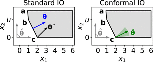
Notes. The shaded areas are the feasible region . The arrow labeled denotes the ground-truth parameter, while the arrows originating at the origin indicate the extreme rays of . The arrows labeled denote the point estimates. In the conformal IO panel, the shaded sector around the point estimate denotes the uncertainty set .
Let the ground truth parameter vector be and , where is a real constant. The optimal solution of corresponding to is point , as shown in Figure 2. Now, suppose is uniformly and independently drawn from for all , resulting in a data set , where . Given the support , the possible decisions in the data set (assuming the solver only returns extreme points) are points , , and . Let , , and be the number of times , , appear in , respectively.
Suppose and (which occurs with probability one as ). Then, the optimal solution to with the suboptimality loss is , where satisfies , corresponding to the arrow orthogonal to Constraint (7b) in Figure 2. This implies that the decision policy derived by solving , , randomly draws from . However, point is suboptimal with respect to and most . It can be shown that (see Online Section EC.1.1 for all calculations) the AOG and POG of are and , respectively, both of which can be arbitrarily large as u increases.
This example shows that with the suboptimality loss can produce a point estimate that deviates from the ground truth and from most realizations . These estimation errors may be amplified in the downstream optimization phase, leading to considerable decision errors as measured by AOG and POG. A similar issue is highlighted in Elmachtoub and Grigas (2022). Existing literature proposes two strategies to tackle this issue: (i) a decision-aware loss function for parameter estimation (Wilder et al. 2019, Mandi et al. 2022) and (ii) a robust optimization model that accounts for the estimation errors (Chan et al. 2023b, Sun et al. 2023). Strategy (i) is not applicable in our setting because of computational tractability and because we do not assume access to observations of the unknown parameters. We propose a new method along the lines of strategy (ii).
3.4. Incorporating Robustness into the Decision Pipeline
In this section, we introduce a new decision policy that uses a robust optimization model for decision prescription (as opposed to using as in the standard IO pipeline). This robust model hedges against deviations from a point estimate, leading to decisions less sensitive to parameter estimation errors. Specifically, we solve the following robust forward optimization problem.
In this model, is an uncertainty set centered at the point estimate with being parameters that control its size. We define
This uncertainty set is the unit spherical cap in , that is, the intersection of the unit sphere and a revolution cone with center and aperture angle .
(
(
3.5. Performance of the Robust Decision Policy: Example Revisited
To illustrate the performance of this new policy, we apply it to the example from Section 3.3. We construct the uncertainty set around obtained by solving the with the suboptimality loss. When the angle satisfies , the optimal solution to is always , which is optimal with respect to and most . It can be shown that (see Online Section EC.1.2) the AOG and POG that result from this pipeline are zero and upper bounded by , respectively, regardless of u. Whereas this pipeline guarantees a bounded AOG and POG in this example, its performance still depends on the choice of , which we address in Section 4.
3.6. The Value of Robustness
We now present theoretical results that formalize the value of incorporating robustness into our decision pipeline. These results identify the conditions under which the policy performs well and motivate our approach for constructing uncertainty sets in the next section. The following lemma is an immediate result of the objective function f being linear in (see Equation (2)).
For any and , there exists a constant such that, for any , we have .
(
Theorem 1 characterizes the performance of our decision policy in terms of AOG and POG when the uncertainty set used for decision prescription can rationalize an unseen, future decision with some probability. To examine the tightness of these bounds, we evaluate their numerical values in Online Section EC.1.3 using the example from Section 3.3, in which the empirical POG and AOG closely match the theoretical bounds. Let be the minimal angle that satisfies the coverage condition in Theorem 1. This choice of ensures that the bounds in Theorem 1 have well-defined derivatives with respect to (because multiple feasible may exist for a given ) and provides additional insight into the comparison between standard IO and our decision policies. After substituting with , the bounds in Theorem 1 become
The POG and AOG bounds at offer several key insights. First, the right-hand derivatives of and at are strictly negative. Because implies and, therefore, recovers the standard IO method, this result shows that introducing even an infinitesimal amount of robustness leads to immediate improvements over standard IO in both guarantees. This underscores the value of robustness in our decision policy as formalized in the next proposition.
(
Second, a reasonable point estimate is essential for realizing the value of robustness. Proposition 1 requires that the point estimate rationalizes a randomly drawn decision with positive probability. That is, the uncertainty set must be centered around a reasonably accurate . This requirement is mild as it is satisfied whenever lies within the support of . Conversely, if is severely inaccurate, both standard IO and our policies are likely to perform poorly.
Third, the performance of our policy may be improved by tuning . Whereas increasing from zero to a small value yields improvements in both bounds, the bounds are not necessarily monotone in because of their dependence on and . So larger values of may sometimes weaken the guarantees. In practice, should, thus, be selected with care, for example, via cross-validation.
Finally, the AOG bound has an additional term , which captures the divergence between the mean perception of the decision makers and the ground truth (see Assumption 2). When , the AOG and POG bounds coincide. However, when the wisdom of the crowd deviates significantly from , learning from the decisions becomes difficult. In such cases, if or an estimate of it is available, we may use the strategy presented in Remark 7 to trade off between AOG and POG.
The , , and values in Theorem 1 are finite. A natural uniform upper bound for them is , where is as defined in Lemma 1. In the special case in which , this reduces to , that is, the largest distance from the origin to any point in .
4. Conformal Inverse Optimization
The theoretical results in Section 3.6 rely on the requirement that parameters in the uncertainty set can rationalize future decisions with a specified probability . In this section, we propose a principled method to construct an uncertainty set that satisfies this requirement asymptotically. Together with the solution of , this method yields a new IO-based decision pipeline. As illustrated in Figure 1, the pipeline has four steps: (i) data splitting, (ii) point estimation, (iii) uncertainty set calibration, and (iv) decision prescription. We refer to the first three steps as conformal inverse optimization because they follow the spirit of conformal prediction (Vovk et al. 2005) and to the overall framework as the conformal IO pipeline. Section 4.1 details the procedure for learning uncertainty sets (steps (i)–(iii)), whereas Section 4.2 introduces an algorithm to accelerate step (iv).
4.1. Learning an Uncertainty Set
4.1.1. Algorithm.
Our approach has the following three steps.
Step i. Data split: We split into training () and validation () sets. Let and index the elements in and , respectively, and and .
Step ii. Point estimation: Given the training set , we solve with the suboptimality loss to obtain a point estimate . Other approaches are possible, such as using a different loss function in or using end-to-end machine learning approaches by treating as an optimization layer that returns a decision based on and applying gradient-based methods, for example, Berthet et al. (2020), to optimize . We compare our approach with these others in Section 5. Note that our uncertainty set calibration method works with any point estimation approach.
Step iii. Uncertainty set calibration: Given a point estimate , we construct an uncertainty set using that, with a specified probability, contains parameters that rationalize the next unseen decision. Note that we can naively achieve a probability of one by setting , but the resulting would generate overly conservative decisions. So we are interested in learning the smallest uncertainty set that achieves the desired probability. The uncertainty set calibration problem is
(
(
Solving appears to be hard because of the nonconvexity of Constraints (10d) and the growth in its size as increases. Nonetheless, we can efficiently solve using the following insights.
Let be a data set, , , and be an operator that returns the largest value in a set. The optimal solution to is with .
Theorem 2 states that we can solve by (i) solving optimization problems whose size is independent of and (ii) finding a quantile in a set of elements. This decomposition helps eliminate Constraint (10c), whose full representation (see Online Section EC.2.6) involves binary variables indicating whether each validation data point is covered by the uncertainty set, which contributes to the intractability of . Step (i) is parallelizable, and step (ii) can be done in time. Because the problem required for evaluating is a maximization problem, we can replace the constraint with if , so this problem is convex when is convex.
4.1.2. Properties of the Learned Uncertainty Set.
(
Moreover, for any , with probability at least , is such that
Theorem 3 states that our learned uncertainty set is conservatively valid and asymptotically exact. Specifically, our method produces a set that contains a that makes the next decision maker’s decision optimal no less than of the time that it is used (conservatively valid). The probability in Inequality (11) is with respect to the joint distribution over and the new sample. Moreover, once the set is given, we have high confidence that the probability of the next decision maker’s decision being covered is within from . The probability in Inequality (12) is with respect to the new sample, whereas the high confidence is with respect to the draw of the validation data set. Overall, we have the almost sure convergence of to as .
4.2. Acceleration Scheme for Prescribing New Decisions
Once an uncertainty set is calibrated and a new context is given, we then solve to prescribe new decisions. In this section, we discuss the computational challenges of solving this problem and methods to accelerate its solution process.
Let , and then can be written as
Note that, in many applications, we know and are both nonnegative. For example, in routing problems in which , the travel costs represented by are typically nonnegative and the routing decisions represented by are binary (Zattoni Scroccaro et al. 2024b). In these cases, we can replace the constraint with , leading to the following reformulation.
Given a fixed , assuming that and for any , then Problem (13) can be formulated as
Going forward, we assume that and are nonnegative. Whereas this reformulation accelerates the solution process, Problem (14) may still be difficult to solve. For example, when involves discrete decisions, Problem (14) is a quadratic mixed integer program. In light of this challenge, we develop an approximation to Problem (14). In particular, we approximate the norm using a polyhedral norm , defined as a norm such that the unit ball is a polyhedron. A benefit of this approach is that we can dualize the inner problem and generate an approximation to with similar computational tractability as . Specifically, we solve
The next proposition bounds the optimality loss of using an optimal solution to (15) as a function of the approximation error of the polyhedral norm to the norm.
Let be a norm that satisfies for any and some , and be optimal solutions to Problems (14) and (15), respectively, and , which is finite because the basis functions are continuous and the feasible set is compact. Assuming that , , and for any , then .
Indeed, the idea of approximating the norm using a polyhedral norm has been used to improve the computational tractability of other norm-constrained optimization models. Existing literature proposes the D-norm (Bertsimas et al. 2004), which approximates a vector’s norm as a weighted sum of its largest entries, and the norm (Chen et al. 2025), which derives an approximation as the maximal inner product of the vector of interest and any vectors that satisfy a set of constraints on their and norms. Whereas both the D-norm and -norm enjoy global bounds on the approximation error, our experiments suggest that their local approximation errors for were large and the resulting decisions were of poor quality. Thus, we propose the following data-driven norm, which can be written as a linear combination of polyhedral norms and whose parameters can be tuned to refine the approximation locally.
(
We require to be nonnegative so is nonnegative. Moreover, it is easy to verify that satisfies the triangle inequality and . So is a norm.
There are many possible norms that could be used to form the data-driven norm, including the , , D-norm, and -norm. We demonstrate in our numerical results that simply using and achieves strong empirical performance, approaching the best possible performance (obtained using an exact algorithm). We write the specific data-driven norm that uses and as
To approximate the norm with , we need to fit the parameters and using data collected around the region of interest, that is, . Generating the training data can be a daunting computational task when is high dimensional. It typically involves (i) generating random vectors in a d-dimensional space and (ii) accepting the vector if it falls inside the specified region. The probability of accepting in step (ii) decreases quickly as the dimensionality increases; see discussions in Arun and Venkatapathi (2025). In response, we build a training set for fitting the data-driven norm using the cost vectors generated in the uncertainty set calibration step, that is, in the solution of (see Section 4.1), which are guaranteed to be around the subregion of interest. The complete procedure is detailed in Online Section EC.3.6. Once the training data are generated, can be fit as a constrained linear regression model with zero intercept. The next corollary specializes the bound in Proposition 3 for the data-driven norm .
For any fixed , , and , let be an optimal solution to Problem (14) and be an optimal solution to Problem (15) with . If and , then
Corollary 1 characterizes the solution quality achieved by our data-driven approximation model. The bound requires to be larger than a threshold. If both and are small, then the resulting polyhedron would be much larger than the unit ball, leading to overly conservative cost estimation for a decision . In principle, one should include this threshold constraint in the parameter estimation problem. However, we find that fitting the regression without this constraint always results in parameters that satisfy the inequality. The intuition is that small generally results in poor approximation error, which is the training loss used for parameter estimation. Additionally, the bound also requires that be below a threshold. If and are too large, the resulting polyhedron would be much smaller than the unit ball, leading to an underestimation of the decision cost. Similarly, we find empirically that our fitted parameters always satisfy this constraint as is the center of the original uncertainty set, around which the data-driven norm typically achieves small approximation errors. Thus, we ignore both constraints so we can use off-the-shelf ML packages to fit . If the parameters violate these constraints, one can simply fit the model again by solving a constrained optimization model with the constraints embedded.
The bound in Corollary 1 provides direct insight into the performance of the general bound. We expect the bound in Proposition 3 to increase as increases, reflecting the fact that it is harder to achieve high approximation accuracy and, thus, high decision quality when the uncertainty set is larger. We also expect the bound to go to zero when goes to zero. But without an explicit relationship between and , these behaviors are difficult to establish. With , Corollary 1 provides a clear picture of the bound’s behavior as a function of : increasing in and converging to zero as goes to zero as expected. Finally, we present a complete formulation of Problem (15) with in Online Section EC.2.11. The model is a linear mixed integer program when is discrete.
5. Numerical Studies
We perform numerical studies with synthetic problem instances to compare the performance of the standard and conformal IO pipelines. Section 5.1 introduces the experimental setup; Section 5.2 presents main numerical results. Additional results regarding the choice of hyperparameters, uncertainty set size, other baselines, and alternative performance metrics are in Online Section EC.4.
5.1. Experiment Setup
We consider two forward problems: (i) a shortest path problem on a grid (linear program) and (ii) a knapsack problem with 10 items (integer program). Inverse models of such problems are studied in the literature (Burton and Toint 1992, Turner and Chan 2013). See Online Section EC.3.2 for formulations. For both problems, we generate a ground truth and a data set of N = 1,000 decisions, corresponding to distinct decision makers. For each decision maker k, we generate for , where is drawn from and is drawn from a standard normal distribution. For the shortest path problem, is a random origin–destination pair. For the knapsack problem, item weights are drawn from [1, 10] and are shared among decision makers. Each decision maker has a budget , where is drawn from .
We focus on comparing conformal IO with the standard IO to highlight the value of incorporating robustness in the decision pipeline. Additional strategies for improving both pipelines are in Online Section EC.4.4. We implement both policies with two point estimation methods: (i) solving with the suboptimality loss, and (ii) the perturbed Fenchel–Young loss approach from Berthet et al. (2020). See Online Section EC.3 for details. In all experiments, our policy uses the training set for point estimation and the validation set for calibration, whereas the standard IO policy uses the union of the training and validation sets for point estimation. Thus, both policies use the same amount of data and are evaluated on the same test set.
5.2. Experiment Results
5.2.1. Uncertainty Set Validity.
We first evaluate the out-of-sample coverage achieved by the uncertainty set learned using conformal IO under different target levels and sample sizes . As shown in Figure 3, when the validation set is small (), we always achieve the specified target, but tends to overcover. When using larger validation sets (), our coverage level gets closer to . These empirical findings echo our theoretical result in Theorem 3.
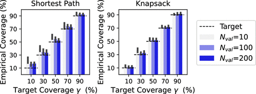
Notes. We evaluate each uncertainty set using 500 out-of-sample data points. Each experiment is repeated 10 times, and we report the average empirical coverage along with the range across the 10 runs (shown as error bars).
5.2.2. Solution Quality.
As shown in Figure 4, conformal IO typically achieves lower POG and AOG. On average, when varying , conformal IO improves the AOG by 20.1%–30.4% and the POG by 15.0%–23.2% for the shortest path problem and improves the AOG by 40.3%–57.0% and the POG by 13.5%–20.1% for the knapsack problem. The solutions generated by conformal IO are not only of higher quality but also perceived to be of higher quality. The performance of conformal IO improves quickly as increases from 0% to 10%, reflecting the value of robustness (recall Proposition 1). It may further improve as increases but can also worsen slightly when becomes large. This finding aligns with Theorem 1, which shows that performance may not vary monotonically with . In practice, this parameter should be tuned via cross-validation.
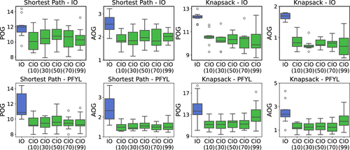
Notes. Each box plot summarizes performance over 10 random 60-20-20 train–validation–test splits of a data set with 1,000 data points. The numbers in parentheses indicate the target coverage level used in the CIO pipeline.
5.2.3. Computational Efficiency.
As shown in Table 1, the two pipelines have similar training times. In standard IO, training refers to generating the point estimate by solving the . In conformal IO, training time is the time it takes to solve both the and . When is an integer program (knapsack), the training of conformal IO is faster as it replaces a relatively large inverse integer program (associated with ), which is notoriously difficult to solve, with a smaller inverse problem and a set of small calibration problems (Theorem 2). For prediction, our method achieves lower AOG and POG at the cost of solving a more challenging . As these problems are small, we can solve them exactly with a cutting plane method described in Online Section EC.3.5.
|

Table 1. Average (Standard Deviation) Computational Time of Standard and Conformal IO Pipelines in Seconds
| Training | Prediction (per decision) | |||
|---|---|---|---|---|
| Problem | Standard IO | Conformal IO | ||
| Shortest path | 0.18 (0.02) | 0.27 (0.03) | 0.01 (0.00) | 0.63 (0.12) |
| Knapsack | 2.47 (0.37) | 1.95 (0.32) | 0.01 (0.00) | 0.44 (0.15) |
Next, we investigate the performance of the data-driven approximation models described in Section 4.2. We focus on the shortest path problem as our approximation requires the cost vector to be nonnegative. As shown in Online Section EC.4.2, our data-driven norm achieves significantly lower approximation errors to the norm than other norms from the literature. Below, we perform computation experiments to study if the reduced approximation error can be translated into better decisions.
5.2.3.1. Trade-off Between Solution Time and Solution Quality.
We compare our data-driven approximation model against approximation models that utilize the D, , , and norms. We also implement the polyhedral outer approximation method from Kocuk (2021). This method can approximate the second order cone described by the norm constraint arbitrarily well with a polyhedral cone in an extended space. The number of additional decision variables and constraints grow polynomially in , where denotes the target approximation error, which we vary in . To obtain the exact solution, we implement the cutting-plane algorithm and the quadratic program reformulation presented in Section 4.2. For each method, we report the average percentage reduction in out-of-sample AOG and POG with respect to the standard IO pipeline (y-axis) and the solution time required to generate 200 routes (x-axis) in Figure 5.

Notes. The small and large instances are on and grids, respectively. The approximation models are omitted as they are far worse than others. The points labeled “Poly Approx,” from left to right, represent implementations of the method of Kocuk (2021) with increasing approximation accuracy.
For small instances, our approach is the only norm-based approximation method that can achieve AOG and POG reductions compared with standard IO. Some of the polyhedral approximation models of Kocuk (2021) can achieve similar AOG and POG reduction but take two to five times as long to solve. The only competitor to our approach for small problem sizes is the exact cutting-plane method, which achieves comparable AOG and POG with similar solution time. For large instances, however, exact approaches were not able to find a feasible solution. In these cases, our data-driven norm approximation model essentially Pareto-dominated the others: (i) it achieved similar solution quality using less than 10% of the solution time compared with the polyhedral approximation model, and (ii) at similar computational expense, it was the only norm-approximation model to achieve AOG and POG reductions. Compared with other norms, the advantage of the data-driven norm lies in the fact that the resulting uncertainty set has more vertices than those defined by its constituent norms, allowing for a closer approximation to the ball. As visualized in Online Section EC.3.7, our data-driven polyhedron (constructed from the and norms) has vertices in , whereas the and balls have 2d and , respectively. This is important as only these vertices can be optimal solutions to the inner problem in . By increasing the number of vertices, we hedge against a broader range of parameter realizations, thereby improving robustness and out-of-sample performance.
5.2.4. Summary.
The main takeaways are that (i) conformal IO generates uncertainty sets that satisfy the target coverage levels, (ii) the conformal IO pipeline produces decisions with higher absolute and perceived quality than standard IO, and (iii) replacing in the conformal IO pipeline with our data-driven norm approximation model significantly enhances its computational tractability, still improving absolute and perceived decision quality compared with standard IO.
6. Case Study
Finally, we present a case study related to delivery path recommendations in Toronto, Canada. The primary goal of food delivery platforms is to fulfill customer demand in a timely manner. However, a theoretical shortest path may be suboptimal from the courier’s perspective. So platforms may need to trade delivery time for path adherence, which impacts many downstream operations, for example, order batching, which relies on accurate route modeling. The question becomes, how much additional travel time must the platform bear to achieve a certain adherence rate? We perform experiments to quantify this trade-off. We focus on bike delivery, which is increasingly popular in urban areas as it is low cost, low emission, and often faster than car delivery (DoorDash 2024).
6.1. Data
6.1.1. Road Network.
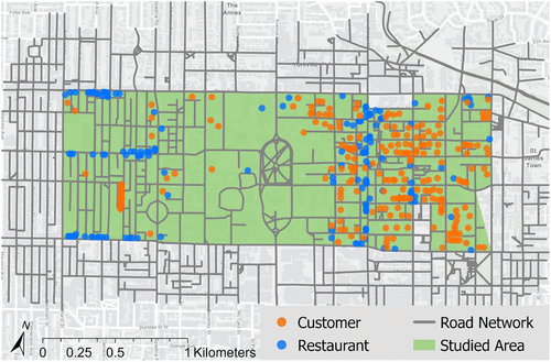
We focus on delivery trips whose origin and destination are within the forward sortation areas M5S and M4Y in Toronto, Canada (Figure 6). We retrieve the road network from City of Toronto (2020) and focus on the subnetwork within 500 meters of the studied area’s boundary so couriers can use segments outside this area. The network is represented as a directed graph , where and are the sets of 1,163 intersections and 2,450 road segments, respectively.
6.1.2. Road Segment Features.
We collect features related to length, traffic volume, and bike friendliness for each edge. The edge lengths are retrieved from the road network. We obtain the daily motor traffic volume on each edge from a well-established transportation model (Travel Modelling Group 2016). We categorize traffic volume into light (≤8,000 vehicles/day), medium (between 8,000 and 20,000 vehicles/day), and heavy volume (≥20,000 vehicles/day) following the route choice model proposed by Zimmermann et al. (2017), which we introduce later. Let and denote if edge has medium or heavy volume, respectively. For bike friendliness, we follow Lin et al. (2021) to classify edges into low- and high-stress based on detailed road network data, including road geometry, traffic speed, and the presence of bike infrastructure. Let denote if edge is high-stress (one) or not (zero).
6.1.3. Perceived Travel Cost.
We consider a set of bike couriers indexed by , each having an unobservable travel cost perception for each edge . We generate travel cost perceptions by adapting a route choice model fitted by Zimmermann et al. (2017). Specifically,
6.1.4. Delivery Routes.
We generate delivery routes for each courier, totaling observed routes. Each route k has an origin and a destination that are, respectively, sampled from 147 restaurants and 230 residential buildings queried from the study area using OpenStreetMap (2017). We ensure that and are at least 1 km apart to justify the use of a food delivery service. We generate a route from to by solving a shortest path problem based on the courier’s perception . We set and vary this value in Section 6.3.3.
6.2. Experimental Setup
6.2.1. Forward Problem.
Given edge features and routes , let be a feature matrix in which each column corresponds to an edge, be the node–edge incidence matrix of graph , and be a vector with a one in the entry corresponding to o and a in the entry corresponding to d with all other entries being zero. Because the travel cost is linear in edge features, we formulate the following multiobjective shortest path problem between o and d as :
6.2.2. Path Evaluation and Prescription.
We assess the recommended paths using POG, a proxy for courier adherence, and AOG with , which reflects the food delivery platform’s preference to prioritize service quality (i.e., delivery time). We consider three policies for path recommendation: (i) the standard IO policy, which relies on a point estimate of ; (ii) a conformal IO policy, which leverages an uncertainty set constructed for ; and (iii) the shortest-path policy that generates paths by solving FOP with . Method (i) mimics the IO method used by Rönnqvist et al. (2017), whereas method (iii) reflects current industry practice. Because is known, we can explicitly trade off between adherence and service quality when applying standard and conformal IO. Specifically, when prescribing a path from o to d, we add a constraint to or , where denotes the vector of edge travel times, is the travel time of the shortest path from o to d, and is the maximum percentage increase in travel time that the platform allows. As increases, we expect the path to achieve a higher adherence rate and lower service quality as the model can operate in a larger feasible region, tailoring the path to the courier’s preferences. We vary from 0% to 20% to provide a spectrum of possible model performance. Note that, when , both the standard and conformal IO policies coincide with the shortest path policy.
6.3. Results
6.3.1. Trade-off Between Path Adherence and Service Quality.
As shown in Figure 7(a), compared with the shortest path policy (point A), conformal IO (point B) can reduce POG by up to 93%, only increasing AOG by 80 units, corresponding to an 8% increase in travel time. For any level of POG reduction, conformal IO consistently incurs a smaller AOG than standard IO. This performance gap widens as increases.
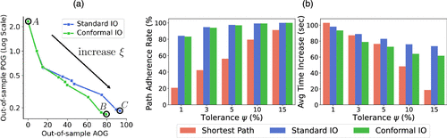
Notes. Panel (a) shows the AOG and POG achieved by the two pipelines when varying . Point A corresponds to the shortest path policy. Points B and C correspond to setting to 20% for the conformal and standard IO pipelines, respectively. Panel (b) shows the path adherence rates and average delivery times achieved at points A, B, and C, when varying couriers’ tolerance for suboptimal recommendations ().
Next, we investigate how the POG reduction translates into improvements in path adherence when the maximum allowed travel time increase from the shortest path is set to for the two IO approaches (points B and C). We assume that couriers follow the recommended path only if it is within % of their perceived optimality. We vary in . As shown in Figure 7(b), for every tolerance level, conformal IO results in a smaller travel time increase compared with standard IO, achieving similar adherence rates. Compared with the shortest path policy, conformal IO achieves significant increases in adherence rates across all values of (e.g., 62.5 percentage points when ). However, the impact on travel times depends on . Most notably, for proud couriers who believe strongly in their own intuition (), there is no trade-off: conformal IO can yield both higher adoption rates and faster deliveries. For humble couriers who have higher tolerance levels (), conformal IO still improves adherence rates by 8.75 to 19.25 percentage points, increasing the travel time by only one to two minutes. Overall, these results highlight the potential to significantly improve path adherence without compromising service quality in last-mile delivery.
The adherence model described above (i.e., adhere if POG is within ) offers a way to quantify the potential real-world impact of our algorithm. We use POG as a predictor for human adherence as empirical studies in human–AI interaction show that individuals are more likely to follow algorithmic recommendations that align with their intuition (Chen et al. 2023, Liu et al. 2023, Bastani et al. 2025). This is particularly salient in last-mile delivery when couriers often view algorithm-proposed routes as low quality and deviate from them (Liu et al. 2021, Merchán et al. 2022, Fu et al. 2023). The threshold structure follows behavioral economics literature (Simon 1955), in which satisficing (i.e., humans choose an action that exceeds an aspiration level) is well studied to model human decision making, and the IO literature (Mohajerin Esfahani et al. 2018), in which -optimality gaps are used to model bounded rationality (i.e., humans may accept suboptimal decisions because of cognitive and computational limitations). Prior work proposes alternative adherence models (see review in Grand-Clément and Pauphilet 2024), but these frameworks are designed to yield analytical insights rather than to support counterfactual evaluation. Our model captures one central driver of adherence in last-mile delivery—alignment with intuition—but we acknowledge that other factors, reviewed in Section 2, also play a role. Some can be modeled in our multiobjective framework (e.g., implementation cost via the bike-friendliness objective in Problem (19)), whereas others, for example, peer influence (Liu et al. 2023), are more difficult to formalize. The improvements above should, thus, be viewed as an optimistic estimate of our algorithm’s impact. As a robustness check, we replicate the experiment with an alternative measure of alignment that accounts for both the gap in perceived optimal value (POG) and the deviation from the perceived optimal decision. The results (Online Section EC.5.1) are consistent with our findings.
6.3.2. Performance Under Misspecification.
One concern of applying IO is model misspecification, meaning the forward problem may not fully capture how decision makers choose their paths. To investigate the performance in such cases, we simulate increasing levels of misspecification by varying in in Equation (18), allowing couriers’ perceived travel costs to depend on higher order interactions between different road features. However, when applying both IO pipelines, we intentionally assume a forward model with . We repeat the experiment in Section 6.3.1 for each value of . As shown in Figure 8, conformal IO consistently provides a better trade-off between path adherence (POG) and delivery efficiency (AOG) than standard IO even when the model is misspecified (). Moreover, the performance gap widens as the level of misspecification increases. This suggests that it is beneficial to use conformal IO in practice as the true forward problem is typically inaccessible, necessitating the use of a wrong model.
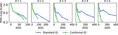
Notes. Each curve is generated by adjusting the maximum allowed percentage increase in travel time, . The y-axis reports the reduction in POG relative to the shortest path policy (rather than raw POG values), allowing all subfigures to share the same scale.
6.3.3. Data Pooling vs. Personalization.
So far, our case study focuses on using one route recommendation model for all couriers, which aligns with current industry practice (Liu and Jiang 2022). An alternative is to personalize recommendations by fitting a separate IO model for each courier based on the courier’s own delivery history. We compare the performance of this strategy (PIO) against standard and conformal IO, both of which use data from multiple users. To understand how data availability affects performance, we vary the number of trips per courier in . As shown in Figure 9, the conformal IO pipeline consistently offers a better trade-off between path adherence and delivery efficiency than standard IO regardless of how much data are available. In the small data regime (), conformal IO significantly outperforms PIO. Therefore, when launching services in a new city or onboarding a new courier in an existing one, it is advantageous to use conformal IO to leverage the shared knowledge from all couriers. In the big data regime, conformal IO performs similarly to PIO. Furthermore, conformal IO incurs lower computational overhead as it requires hyperparameter tuning and model training for only one model across all users, whereas PIO requires separate processes for each courier.
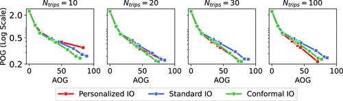
Note. Each curve is generated by adjusting the maximum allowed percentage increase in travel time, .
6.3.4. Summary.
Our results highlight the potential to improve delivery path adherence without compromising service quality in last-mile delivery. Conformal IO has robust performance under model misspecification. It is particularly useful in the small data regime, for example, when the platform is launching services in a new city or onboarding a new courier. In the big data regime, conformal IO closely matches the performance of PIO and requires less computational overhead.
7. Conclusion
In this paper, we propose conformal IO, a new approach for recommending high-quality decisions that align with human intuition. We present the first method for learning uncertainty sets from decision data, which is then utilized in a robust model to prescribe new decisions. Under mild conditions, we prove that conformal IO achieves bounded optimality gaps with respect to both the ground truth parameters and human perceptions. This suggests that decisions based on conformal IO may be more likely to be adopted compared with decisions from standard IO. We demonstrate strong performance of conformal IO using synthetic problem instances and a case study.
The authors are grateful to the area editor, the associate editor, and two referees for their valuable feedback and insightful comments.
References
- (2001) Inverse optimization. Oper. Res. 49(5):771–783.Link, Google Scholar
- (2025) An algorithm for generating uniform random vectors in n-dimensional cones. Sankhya A 87:327–348.Crossref, Google Scholar
- (2018) Inverse optimization with noisy data. Oper. Res. 66(3):870–892.Link, Google Scholar
- (2019) Data-driven incentive design in the Medicare shared savings program. Oper. Res. 67(4):1002–1026.Abstract, Google Scholar
- (2020) Knowledge-based automated planning with three-dimensional generative adversarial networks. Medical Phys. 47(2):297–306.Crossref, Google Scholar
- (2018) An online-learning approach to inverse optimization. Preprint, submitted October 30, https://arxiv.org/abs/1810.12997.Google Scholar
- (2025) Improving human sequential decision making with reinforcement learning. Management Sci. 72(1):733–755.Link, Google Scholar
- (1999) Robust solutions of uncertain linear programs. Oper. Res. Lett. 25(1):1–13.Crossref, Google Scholar
- (2000) Robust solutions of linear programming problems contaminated with uncertain data. Math. Programming 88:411–424.Crossref, Google Scholar
- (2020) Learning with differentiable perturbed optimizers. Adv. Neural Inform. Processing Systems, vol. 33 (Curran Associates Inc., Red Hook, NY), 9508–9519.Google Scholar
- (2004) The price of robustness. Oper. Res. 52(1):35–53.Link, Google Scholar
- (2018) Data-driven robust optimization. Math. Programming 167:235–292.Crossref, Google Scholar
- (2015) Data-driven estimation in equilibrium using inverse optimization. Math. Programming 153:595–633.Crossref, Google Scholar
- (2004) Robust linear optimization under general norms. Oper. Res. Lett. 32(6):510–516.Crossref, Google Scholar
- (2025) Contextual inverse optimization: Offline and online learning. Oper. Res. 73(1):424–443.Link, Google Scholar
- (2022a) Stochastic inverse optimization. Accessed January 20, 2024, https://perma.cc/8T8L-MZZE.Google Scholar
- (2022b) Spatial price integration in commodity markets with capacitated transportation networks. Oper. Res. 70(3):1739–1761.Link, Google Scholar
- (1992) On an instance of the inverse shortest paths problem. Math. Programming 53(1):45–61.Crossref, Google Scholar
- (2020) A systematic review of algorithm aversion in augmented decision making. J. Behav. Decision Making 33(2):220–239.Crossref, Google Scholar
- (2020) Inverse optimization for the recovery of constraint parameters. Eur. J. Oper. Res. 282(2):415–427.Crossref, Google Scholar
- (2019) Inverse optimization: Closed-form solutions, geometry, and goodness of fit. Management Sci. 65(3):1115–1135.Link, Google Scholar
- (2023a) Inverse optimization: Theory and applications. Oper. Res. 73(2):1046–1074.Link, Google Scholar
- (2014) Generalized inverse multiobjective optimization with application to cancer therapy. Oper. Res. 62(3):680–695.Link, Google Scholar
- (2023b) Got (optimal) milk? Pooling donations in human milk banks with machine learning and optimization. Manufacturing Service Oper. Management 27(6):1721–1739.Link, Google Scholar
- (2025) Combining forecasts from multiple experts for multiple variables. Management Sci. 72(8):6542–6558.Link, Google Scholar
- (2023) Understanding the role of human intuition on reliance in human-AI decision-making with explanations. Proc. ACM Human-Comput. Interaction, vol. 7, 1–32.Google Scholar
- (2025) Robust data-driven CARA optimization. Preprint, submitted February 24, https://doi.org/10.2139/ssrn.5130565.Google Scholar
- (2022) Data-driven conditional robust optimization. Adv. Neural Inform. Processing Systems, vol. 35, 9525–9537.Google Scholar
- (2022) Interpretable optimal stopping. Management Sci. 68(3):1616–1638.Link, Google Scholar
City of Toronto (2020) City of Toronto open data. Accessed September 15, 2020, https://open.toronto.ca/.Google Scholar- (2010) Distributionally robust optimization under moment uncertainty with application to data-driven problems. Oper. Res. 58(3):595–612.Link, Google Scholar
- (2018) Overcoming algorithm aversion: People will use imperfect algorithms if they can (even slightly) modify them. Management Sci. 64(3):1155–1170.Link, Google Scholar
- (2021) Wasserstein distributionally robust inverse multiobjective optimization. Proc. AAAI Conf. Artificial Intelligence, vol. 35, 5914–5921.Google Scholar
- (2018) Generalized inverse optimization through online learning. Adv. Neural Inform. Processing Systems, vol. 31.Google Scholar
DoorDash (2024) Bike delivery strategies. Accessed June 12, 2024, https://perma.cc/M98U-A8LC.Google Scholar- (2022) Smart “predict, then optimize.” Management Sci. 68(1):9–26.Link, Google Scholar
- (2023) Learning for guiding: A pairwise inverse reinforcement learning framework for last-mile deliveries. Preprint, submitted November 30, https://doi.org/10.2139/ssrn.4639706.Google Scholar
- (2023) Distributionally robust stochastic optimization with Wasserstein distance. Math. Oper. Res. 48(2):603–655.Link, Google Scholar
Global Times (2021) Panicked woman rider jumps out of car, breaking bones; car-hailing platform probed. Accessed August 1, 2024, https://www.globaltimes.cn/page/202106/1226697.shtml.Google Scholar- (2023) Data-driven robust optimization using deep neural networks. Comput. Oper. Res. 151:106087.Crossref, Google Scholar
- (2024) The best decisions are not the best advice: Making adherence-aware recommendations. Management Sci. 72(1):667–692.Link, Google Scholar
- (1955) Cardinal welfare, individualistic ethics, and interpersonal comparisons of utility. J. Political Econom. 63(4):309–321.Crossref, Google Scholar
- (2021) Learning-based robust optimization: Procedures and statistical guarantees. Management Sci. 67(6):3447–3467.Link, Google Scholar
- (2022) DeepETA: How Uber predicts arrival times using deep learning. Uber engineering blog. Accessed January 19, 2024, https://perma.cc/VBR7-E37Z.Google Scholar
- (2021) When will workers follow an algorithm? A field experiment with a retail business. Management Sci. 67(3):1670–1695.Link, Google Scholar
- (2020) Field experiment on the profit implications of merchants’ discretionary power to override data-driven decision-making tools. Management Sci. 66(11):5182–5190.Link, Google Scholar
- (2016) How much information? Effects of transparency on trust in an algorithmic interface. Proc. 2016 CHI Conf. Human Factors Comput. Systems, 2390–2395.Google Scholar
- (2021) Rational polyhedral outer-approximations of the second-order cone. Discrete Optim. 40:100643.Crossref, Google Scholar
- (2021) The impact of COVID-19 cycling infrastructure on low-stress cycling accessibility: A case study in the City of Toronto. Findings.Crossref, Google Scholar
- (2022) Personalized route recommendation for ride-hailing with deep inverse reinforcement learning and real-time traffic conditions. Transportation Res. Part E Logist. Transportation Rev. 164:102780.Crossref, Google Scholar
- (2021) On-time last-mile delivery: Order assignment with travel-time predictors. Management Sci. 67(7):4095–4119.Link, Google Scholar
- (2024) Planning bike lanes with data: Ridership, congestion, and path selection. Management Sci. 71(9):7631–7654.Link, Google Scholar
- (2023) Algorithm aversion: Evidence from ridesharing drivers. Management Sci. 72(1):193–203.Link, Google Scholar
- (2025) Fat tails in human judgment: Empirical evidence and implications for the aggregation of estimates and forecasts. Management Sci. 72(3):2364–2379.Link, Google Scholar
- (2022) Decision-focused learning: Through the lens of learning to rank. Internat. Conf. Machine Learn. (PMLR), 14935–14947.Google Scholar
- (2025) Human agency in last mile delivery. https://perma.cc/6XM7-7ZJE.Google Scholar
- (2022) 2021 Amazon last mile routing research challenge: Data set. Transportation Sci. 58(1):8–11.Link, Google Scholar
- (2018) Data-driven inverse optimization with imperfect information. Math. Programming 167:191–234.Crossref, Google Scholar
OpenStreetMap (2017) Planet dump. https://planet.osm.org.Google Scholar- (2017) Calibrated route finder: Improving the safety, environmental consciousness, and cost effectiveness of truck routing in Sweden. Interfaces 47(5):372–395.Link, Google Scholar
- (2025) A survey of contextual optimization methods for decision-making under uncertainty. Eur. J. Oper. Res. 320(2):271–289.Crossref, Google Scholar
- (2022) Quantile inverse optimization: Improving stability in inverse linear programming. Oper. Res. 70(4):2538–2562.Link, Google Scholar
- (2017) Data-driven robust optimization based on kernel learning. Comput. Chemical Engrg. 106:464–479.Crossref, Google Scholar
- (1955) A behavioral model of rational choice. Quart. J. Econom. 69(1):99–118.Crossref, Google Scholar
- (2023) Predict-then-calibrate: A new perspective of robust contextual LP. Adv. Neural Inform. Processing Systems, vol. 36, 17713–17741.Google Scholar
- (2022) Predicting human discretion to adjust algorithmic prescription: A large-scale field experiment in warehouse operations. Management Sci. 68(2):846–865.Link, Google Scholar
Travel Modelling Group (2016) GTAModel V4 introduction. Accessed November 20, 2020, https://perma.cc/7CUU-BMHB.Google Scholar- (2013) Examining the LEED rating system using inverse optimization. J. Solar Energy Engrg. 135(4):040901.Crossref, Google Scholar
- (2005) Algorithmic Learning in a Random World, vol. 29 (Springer).Google Scholar
- (2026) The human-AI-human newsvendor: Behavioral biases, partial adherence and learning. Preprint, submitted January 22, https://doi.org/10.2139/ssrn.5999076.Google Scholar
- (2025) Dispatch or hold? An inverse optimization and reinforcement learning approach for multi-objective on-demand delivery. Preprint, submitted December 1, https://doi.org/10.2139/ssrn.5839702.Google Scholar
- (2018) Modeling crew itineraries and delays in the national air transportation system. Transportation Sci. 52(5):1276–1296.Link, Google Scholar
- (2019) Melding the data-decisions pipeline: Decision-focused learning for combinatorial optimization. Proc. AAAI Conf. Artificial Intelligence, vol. 33, 1658–1665.Google Scholar
- (2019) Understanding the effect of accuracy on trust in machine learning models. Proc. 2019 CHI Conf. Human Factors Comput. Systems, 1–12.Google Scholar
- (2023) Inverse optimization and its applications in measuring clinical pathway concordance. Unpublished PhD thesis, University of Toronto, Ontario.Google Scholar
- (2024a) Learning in inverse optimization: Incenter cost, augmented suboptimality loss, and algorithms. Oper. Res. 73(5):2661–2679.Link, Google Scholar
- (2024b) Inverse optimization for routing problems. Transportation Sci. 59(2):301–321.Link, Google Scholar
- (2017) Bike route choice modeling using GPS data without choice sets of paths. Transportation Res. Part C Emerging Tech. 75:183–196.Crossref, Google Scholar
Timothy C. Y. Chan is the associate vice-president and vice-provost, strategic initiatives, and a professor in the department of mechanical and industrial engineering at the University of Toronto. His primary research interests are in operations research, optimization, and applied machine learning with applications in healthcare, medicine, sustainability, and sports.
Erick Delage is a professor in the department of decision sciences at HEC Montréal, where he holds the chair in data-driven decision making. He is a member of the College of New Scholars, Artists and Scientists of the Royal Society of Canada. His research interests span areas of robust and stochastic optimization, decision analysis, reinforcement learning, and risk management with applications to portfolio optimization/option hedging, inventory management, energy, and transportation problems.
Bo Lin is an assistant professor at the National University of Singapore. His research focuses on developing machine learning and optimization methods to evaluate, design, and help people interact with urban systems. Motivated by practical challenges in real-world deployment, the other line of his research integrates machine learning and optimization, aiming to improve the efficiency, effectiveness, and applicability of data-driven decision-making tools.

