Proper and Consistent Production Tradeoffs in Models of Data Envelopment Analysis

1. Introduction

Most models of data envelopment analysis (DEA) are used to assess the efficiency of decision-making units (DMUs) on a selected set of inputs and outputs without taking into account the relative value of individual inputs for the production process and the complexity of producing individual outputs. This leads to a common situation in which DMUs that excel on some relatively insignificant measures (inputs and outputs) may be shown as technically efficient, even if they do not perform well on the remaining technologically more important measures.

1.1. Production Tradeoffs and Weight Restrictions

For the conventional constant and variable returns-to-scale (CRS and VRS) models, introduced to DEA by Charnes et al. (1978) and Banker et al. (1984), information about the relative value of inputs and outputs in the production process can be specified in two mutually dual ways. In the multiplier CRS and VRS models, this takes on the form of restrictions on the input and output weights, or weight restrictions—see, for example, Allen et al. (1997). In the envelopment CRS and VRS models, the weight restrictions are restated in the dual forms as production tradeoffs, which are interpretable as simultaneous changes to the inputs and outputs that are technologically possible at any DMU in the technology (Podinovski 2004).

The specification of technologically realistic production tradeoffs or weight restrictions leads to a meaningful (explainable by the assumptions made) expansion of the CRS or VRS production technology and improved discrimination on efficiency of the models based on them. The use of such tradeoffs and weight restrictions in different models has been reported in various application contexts, including primary healthcare provision (Amado and Santos 2009, Capeletti et al. 2024), school education (Khalili et al. 2010, Podinovski et al. 2024), courts of justice (Santos and Amado 2014), agricultural farms (Atici and Podinovski 2015), labor inspectorates (Santos et al. 2020), railway traffic control centers (Roets et al. 2018), industrial robots (Ravanos and Karagiannis 2023), bank branches (Razipoor-GhalehJough et al. 2020), and electricity distributors (Santos et al. 2011).

As earlier applications of DEA showed, the incorporation of weight restrictions in multiplier DEA models may lead to their infeasibility (Allen et al. 1997, Thanassoulis et al. 2008), in which case the weight restrictions are unusable and need to be reassessed. Podinovski and Bouzdine-Chameeva (2013) proved that the infeasibility of multiplier VRS and CRS models with weight restrictions corresponds to the case in which the dual production tradeoffs expand the technology in such a way that it includes either free (with a zero input) or unlimited production of some nonzero output vector. Furthermore, free or unlimited production does not necessarily manifest itself in an infeasible multiplier model and may remain undetected in the evaluation of efficiency of DMUs.

Free and unlimited production is disallowed by production theory (Färe et al. 1985). Podinovski and Bouzdine-Chameeva (2013) introduced the notion of consistent weight restrictions and tradeoffs as those that do not generate free and unlimited production in the VRS and CRS technologies and develop computational and analytical tests of their consistency. If the tradeoffs are inconsistent, then they should not be used because the expanded VRS or CRS technology and its production frontier are theoretically unsubstantiated. In this case, we need to reconsider the tradeoffs or weight restrictions.

1.2. Motivation and Contribution

In this paper, we show that the requirement of consistency may fail to detect another potential problem with production tradeoffs, which would require correction in any practical application. (The main definitions, models, and tests developed in this paper are naturally introduced in the language of tradeoffs, but they can equivalently be restated in terms of dual weight restrictions.) Namely, we call the specified set of production tradeoffs proper if none of their combinations can lead to an improvement in some inputs and outputs (i.e., a reduction of inputs and increase in outputs) without simultaneously worsening some other inputs and outputs. Otherwise, the tradeoffs are not proper.

It is clear why the tradeoffs should be proper. If they are not, then every DMU in the technology (at least those with strictly positive inputs and outputs) can be improved on some inputs and outputs “for free” without having to become worse on the other measures. This implies that no DMU in the technology can be efficient, which is unrealistic and means that we made an error in the specification of tradeoffs.

We show that production tradeoffs (and weight restrictions) can be consistent but not proper and, similarly, proper but inconsistent. Because both are problematic and require reassessing, in addition to the known tests of consistency, in this paper we develop analytical and computational tests for proper tradeoffs and weight restrictions. We prove that the multiplier VRS or CRS program with not proper weight restrictions either is infeasible or, if it is feasible, assigns a zero weight to all inputs and outputs that, according to the specified tradeoffs, can be improved “for free” in all its feasible (and, therefore, in all optimal) solutions.

We further identify a large and practically important class of production tradeoffs (and weight restrictions), for which it is sufficient to test only if the tradeoffs are proper because this would imply that they are also consistent. (It is worth noting that the tests developed in this paper for proper tradeoffs are also conceptually and computationally simpler than similar tests for consistent tradeoffs, which offers further theoretical and practical advantages.) However, if the specified tradeoffs are not in this class, we generally need to perform both tests.

1.3. Proper Tradeoffs in Decision Analysis

The notion of proper tradeoffs introduced in this paper in the framework of DEA and related mathematical results allow a straightforward interpretation in the terminology of multicriteria decision analysis (MCDA). In this interpretation, the input and output measures in DEA correspond to criteria in MCDA that the decision-maker wishes to minimize and maximize, respectively.

There is significant literature in the field of MCDA devoted to the assessment of tradeoffs between different criteria—see, for example, Keeney and Raiffa (1976). A tradeoff represents a judgement that balances out an improvement on some criteria at the expense of detriment to some other criteria. Often, such information is incomplete and imprecise and is stated in the dual form as a set of linear inequalities in terms of criterion weights (Hazen 1986, Weber 1987, Harju et al. 2019).

Several tradeoffs can be applied collectively, creating complex substitutions involving multiple criteria. If there is some inconsistency, then it is possible that a “collective” tradeoff may represent improvements to only some criteria, without any detriment to the other criteria. In this paper, we call sets of judgements that can create such tradeoffs not proper and develop analytical and computational tests for their identification.

As follows from our main results obtained in Section 4 (stated in terminology of DEA but equally applicable to MCDA), any criterion whose improvement in at least one “collective” tradeoff appears without a detriment to at least some of the other criteria would necessarily have a zero weight in any weighting scheme based on the given set of tradeoffs. This means that any such criterion is effectively excluded from the ranking of decision alternatives, which should be highlighted as possibly based on erroneous judgements that need reassessing.

1.4. Organization of This Paper

The structure of this paper is as follows. In Sections 2 and 3, we briefly outline the known definitions and results concerning production tradeoffs and their consistency. In Section 4, we define proper production tradeoffs, give their dual characterization in terms of weight restrictions, and develop computational and analytical tests for proper tradeoffs. In Section 5, we establish a relationship between proper and consistent tradeoffs for different types of tradeoffs. In Section 6, we give examples that illustrate theoretical results and tests developed in our paper. In Section 7, we consider an illustrative application in the context of research-intensive universities in the United Kingdom. Section 8 contains concluding discussion. The proofs of all mathematical statements are given in Appendix A. In Appendix B, we present detailed statements of several linear programs discussed in the main sections.

2. Production Tradeoffs

Consider technology $\mathcal{T}\subset {\mathbb{R}}_{+}^m\times {\mathbb{R}}_{+}^s$ characterized by $m\ge 1$ inputs and $s\ge 1$ outputs. Decision making units are elements of $\mathcal{T}$ stated as pairs $(\mathbf{x},\mathbf{y})$, where $\mathbf{x}\in {\mathbb{R}}_{+}^m$ and $\mathbf{y}\in {\mathbb{R}}_{+}^s$ are the vectors of inputs and outputs, respectively.

Let $\mathrm{\Omega }$ be the set of observed DMUs (the data set) $({\mathbf{x}}_j,{\mathbf{y}}_j)$, $j\in \{1,\dots ,n\}=\mathcal{J}$. We assume that ${\mathbf{x}}_j\ne \mathbf{0}$ and ${\mathbf{y}}_j\ne \mathbf{0}$ for all $j\in \mathcal{J}$, that is, that each observed DMU has at least one strictly positive input and output.

The VRS technology ${\mathcal{T}}_{\text{VRS}}$ of Banker et al. (1984) generated by the set of observed DMUs $\mathrm{\Omega }$ is stated as the set of all DMUs $(\mathbf{x},\mathbf{y})$ defined by the following conditions:

Removing the normalizing equality ${\mathbf{1}}^{\top }\mathit{\lambda }=1$ from the conditions (1), we obtain a statement of the CRS technology ${\mathcal{T}}_{\text{CRS}}$ of Charnes et al. (1978).

For both CRS and VRS technologies, Podinovski (2004) defines a production tradeoff as a pair of vectors of sign-free components

that represents simultaneous changes to the inputs and outputs assumed technologically possible for any DMU in the technology, provided that all inputs and outputs of the resulting DMU remain nonnegative. Components of vectors $\mathbf{p}$ and $\mathbf{q}$ represent changes to individual inputs and outputs and can be positive, negative, or equal to zero.

Example 1.

Let DMUs be similar academic departments of different universities, for example, business schools. Let the vector of inputs be $\mathbf{x}={(x_1,x_2)}^{\top }$, where $x_1$ is the number of academic staff who teach and do research and $x_2$ is research staff who do research only. Let the vector of outputs be $\mathbf{y}={(y_1,y_2,y_3)}^{\top }$, where $y_1$ and $y_2$ are, respectively, the numbers of undergraduate (UG) and postgraduate (PG) students and $y_3$ is the number of published papers.

In the described setting, we may identify several production tradeoffs. For example, we may assume that the teaching of one UG student does not require more resources than the teaching of one PG student. Therefore, no department should claim extra resources (namely, academic and research staff) if they are required to teach one UG student instead of one PG student. This is expressed by the tradeoff $({\mathbf{p}}_1,{\mathbf{q}}_1)$, where

In this statement, the components of vector ${\mathbf{q}}_1$ specify a reduction of the number of PG students by 1 and a simultaneous increase in the UG numbers by 1, whereas the zero vector ${\mathbf{p}}_1$ means that such change is possible without any change to the academic and research staff.

We may also judge that one additionally employed academic member of staff should be able to teach, for example, at least 10 UG students and publish one paper per year. We state this by the tradeoff $({\mathbf{p}}_2,{\mathbf{q}}_2)$, where

Finally, suppose that the reduction of one research staff should in most cases not lead to the reduction of more than five papers per year. This is expressed by the tradeoff $({\mathbf{p}}_3,{\mathbf{q}}_3)$, where

Suppose that we have specified $K\ge 1$ production tradeoffs, which we state as follows:

Because, as assumed, changing the inputs and outputs of any DMU $(\mathbf{x},\mathbf{y})$ by any of the tradeoffs (5) leads to another DMU that is technologically possible, we can subsequently modify the resulting DMU by the same or another tradeoff, and so on. Allowing for fractional proportions ${\pi }_k\ge 0$, $k\in \mathcal{K}$, in which the tradeoffs in (5) are used, we finally obtain the following DMU:

If all components of vectors ${\mathbf{x}}^{\prime }$ and ${\mathbf{y}}^{\prime }$ are nonnegative, then the DMU $({\mathbf{x}}^{\prime },{\mathbf{y}}^{\prime })$ is technologically feasible and should be included in the model of technology.

Podinovski (2004) defines the VRS technology expanded by production tradeoffs (5) as the smallest technology (in the sense of the minimum extrapolation principle of Banker et al. 1984) that is freely (strongly) disposable, convex and incorporates the stated tradeoffs. An operational statement of this technology is given by the following conditions:

Similarly, an extension of the CRS technology ${\mathcal{T}}_{\text{CRS}}$ by production tradeoffs (5) is defined by the axioms of technology ${\mathcal{T}}_{\text{VRS}-\text{TO}}$ and the additional axiom of scalability, referred to as “ray unboundedness” by Banker et al. (1984). Such extended CRS technology ${\mathcal{T}}_{\text{CRS}-\text{TO}}$ is obtained from the statement (6) by removing the equality ${\mathbf{1}}^{\top }\mathit{\lambda }=1$.

Example 2.

Consider the VRS technology with a single input x and single output y defined by three observed DMUs A, B, and C in Figure 1. This technology is shown as the darker shaded area below and to the right of the line KABL. Further consider the two production tradeoffs:

$$(p_1,q_1)=(-1,-1),\hspace{1em}(p_2,q_2)=(2,0.5).$$(7)

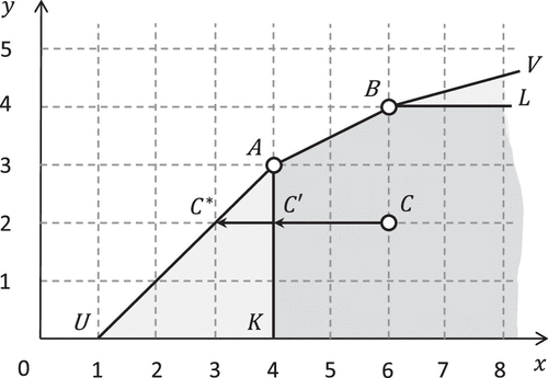
The specification of these two tradeoffs adds the lighter shaded areas UAK and LBV to the technology. For example, the new DMU $C^{*}$ is obtained if we apply the tradeoff $(p_1,q_1)=(-1,-1)$ to the observed DMU A. Applying this tradeoff three times (with ${\pi }_1=3$ in the above notation), we obtain DMU U. Similarly, the line BV is obtained by modifying DMU B by the tradeoff $(p_2,q_2)$ taken in varying proportions ${\pi }_2\ge 0$.

The VRS model based on the expanded technology ${\mathcal{T}}_{\text{VRS}-\text{TO}}$ exhibits a better discriminating power than the original VRS model based on technology ${\mathcal{T}}_{\text{VRS}}$. Indeed, in the latter, the input projection of the inefficient DMU C is DMU $C^{\prime }$, and the input radial efficiency of DMU C is equal to $4/6=2/3$. In the expanded technology, the input projection of DMU C is DMU $C^{*}$, and the input radial efficiency of DMU C is reduced to $3/6=1/2$.

The statement of envelopment models for the assessment of efficiency of DMUs in technologies ${\mathcal{T}}_{\text{VRS}-\text{TO}}$ and ${\mathcal{T}}_{\text{CRS}-\text{TO}}$, which may employ different measures of efficiency, is straightforward. Examples of such efficiency measures include the input and output radial measures of efficiency employed by Charnes et al. (1978) and Banker et al. (1984), measures based on directional distance functions of Chambers et al. (1998) and various nondirectional and slack-based measures, such as those developed by Tone (2001), Fukuyama and Weber (2009), and Färe and Grosskopf (2010).

Dual to the envelopment models are multiplier models stated in terms of vectors of input and output weights $\mathbf{v}\in {\mathbb{R}}_{+}^m$ and $\mathbf{u}\in {\mathbb{R}}_{+}^s$ and, in the case of VRS, the sign-free variable $u_0$ that is dual to the normalizing equality ${\mathbf{1}}^{\top }\mathit{\lambda }=1$.

Podinovski (2004) showed that the specification of tradeoffs (5) in envelopment models is equivalent (in the sense of duality) to the incorporation of the following weight restrictions in the multiplier models:

As an illustration, let ${(v_1,v_2)}^{\top }$ and ${(u_1,u_2,u_3)}^{\top }$ be the vectors of input and output weights in the setting considered in Example 1. The specification of tradeoffs (2)–(4) in envelopment VRS and CRS models is equivalent to the incorporation of the following weight restrictions in their dual multiplier models: $u_1-u_2\le 0$, $10u_1+u_3-v_1\le 0$ and $-5u_3+v_2\le 0$.

Remark 1.

The duality of tradeoffs (5) and weight restrictions (8) allows us to give an interpretation of production tradeoffs in terms of marginal characteristics of production frontiers such as marginal productivity and rates of transformation and substitution between inputs and outputs. As a simple example, consider technology ${\mathcal{T}}_{\text{VRS}-\text{TO}}$ in Example 2, which incorporates tradeoffs (7). According to (8), the latter can be restated in the dual form as the weight restrictions $-u_1+v_1\le 0$ and $0.5u_1-2v_1\le 0$ or as the two-sided inequality

$$0.25\le \frac{v_1}{u_1}\le 1.$$(9)

For any optimal solution of the multiplier model based on technology ${\mathcal{T}}_{\text{VRS}-\text{TO}}$, the ratio of optimal weights $v_1^{*}/u_1^{*}$ is equal to the marginal productivity on the supporting hyperplane to the technology whose equation (in the input and output dimensions x and y) is $-x{v}_1^{*}+y{u}_1^{*}+u_0^{*}=0$. (For the standard VRS technology, this was shown by Banker et al. (1984). For arbitrary polyhedral technologies, including the VRS and CRS technologies with tradeoffs, this was proved by Podinovski and Bouzdine-Chameeva (2021). The formula for marginal productivity then follows from the implicit function theorem.)

The two-sided inequality (9) and the underlying tradeoffs (5) state that the production frontier enveloping the data must have the marginal productivity in the range between 0.25 and 1. This technology is depicted in Figure 1. The highest marginal productivity equal to 1 is observed on the supporting hyperplane that includes the segment UA. The lowest marginal productivity equal to 0.25 is observed on the supporting hyperplane that includes the line BV. Any other supporting hyperplane to the technology has the marginal productivity strictly in the range [0.25, 1]. For example, it is equal to 0.5 on the segment AB.

3. Consistent Production Tradeoffs

In this section, we briefly outline the notion of consistent tradeoffs and weight restrictions introduced by Podinovski and Bouzdine-Chameeva (2013, 2015). We use this outline to contrast consistent tradeoffs with the new notion of proper tradeoffs introduced in Section 4.

The specification of production tradeoffs (5) or weight restrictions equivalent to them (8) expands technologies ${\mathcal{T}}_{\text{VRS}}$ and ${\mathcal{T}}_{\text{CRS}}$ to the generally larger technologies ${\mathcal{T}}_{\text{VRS}-\text{TO}}$ and ${\mathcal{T}}_{\text{CRS}-\text{TO}}$. In some cases, the expanded technology may become unrealistically large and no longer comply with the basic axioms of production theory (see, e.g., Färe et al. 1985). This means that the tradeoffs and the expanded technology based on them are theoretically unsubstantiated.

Podinovski and Bouzdine-Chameeva (2013, 2015) identified a case in which the expanded technologies ${\mathcal{T}}_{\text{VRS}-\text{TO}}$ and ${\mathcal{T}}_{\text{CRS}-\text{TO}}$ allowed either free or unlimited production of a nonzero output vector (we define this formally below), which is disallowed by production theory and indicates an error in the specification of production tradeoffs. This leads to the notion of consistent production tradeoffs (and weight restrictions dual to them) whose specification does not result in free and unlimited production.

Definition 1.

Let ${\mathbf{y}}_o$ be a nonzero output vector, that is, ${\mathbf{y}}_o\in {\mathbb{R}}_{+}^s\backslash \{\mathbf{0}\}$. Technology $\mathcal{T}$ allows free production of vector ${\mathbf{y}}_o$ if $(\mathbf{0},{\mathbf{y}}_o)\in \mathcal{T}$. Technology $\mathcal{T}$ allows unlimited production of ${\mathbf{y}}_o$ if there exists an input vector ${\mathbf{x}}_o\in {\mathbb{R}}_{+}^m$ such that $({\mathbf{x}}_o,\alpha {\mathbf{y}}_o)\in \mathcal{T}$ for all $\alpha \ge 0$.

It is clear that the standard VRS and CRS technologies based on a finite set of observed DMUs do not allow free and unlimited production. However, their extensions by tradeoffs may generate such production; see Example 3 below.

Definition 2.

Production tradeoffs (5) are consistent with technology ${\mathcal{T}}_{\text{VRS}}$ (or with technology ${\mathcal{T}}_{\text{CRS}}$) generated by the data set of observed DMUs $\mathrm{\Omega }$ if the expanded technology ${\mathcal{T}}_{\text{VRS}-\text{TO}}$ (respectively, ${\mathcal{T}}_{\text{CRS}-\text{TO}}$) does not allow free and unlimited production. Otherwise, the tradeoffs (5) are inconsistent with technology ${\mathcal{T}}_{\text{VRS}}$ (or, respectively, ${\mathcal{T}}_{\text{CRS}}$).

As shown by Podinovski and Bouzdine-Chameeva (2013), the consistency of production tradeoffs generally depends on the set of observed DMUs $\mathrm{\Omega }$. Namely, the tradeoffs (5) may be consistent with the VRS or CRS technology generated by one data set and inconsistent with these technologies generated by another data set.

Example 3.

Consider a modification of Example 2 in which we use the same tradeoffs (7) but employ a modified set of observed DMUs A, B, and C. Figure 2 shows the standard VRS technology as the darker shaded area below and to the right of the line KABL. Let us show that although we employ the same tradeoffs as in Example 2, these tradeoffs are no longer consistent with the technology (which is generated by a different data set).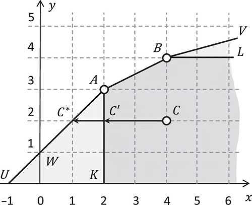

Indeed, if we modify DMU A by the tradeoff $(p_1,q_1)$ taken in proportion ${\pi }_1=2$, we obtain DMU W, which represents free production. (The input of DMU W is equal to zero, and its output is equal to one.) Note that free production caused by the specification of tradeoff $(p_1,q_1)$ is not easily observed by the standard assessment of efficiency. Indeed, in Figure 2, DMU C is projected on DMU $C^{*}$, and its input radial efficiency is equal to $1/4$, which may not appear as problematic. Below, we discuss how the consistency of tradeoffs (5) can be rigorously tested.

As proven by Podinovski and Bouzdine-Chameeva (2013), production tradeoffs (5) are consistent with the VRS technology generated by a set of observed DMUs $\mathrm{\Omega }$ if and only if they are consistent with the CRS technology generated by the same data set. Therefore, we can simply state that the tradeoffs (5) are consistent or inconsistent with the data set $\mathrm{\Omega }$ without referring to the VRS or CRS technology. It further turns out that the inconsistency of tradeoffs manifests itself differently in the two technologies. In the CRS technology, inconsistent tradeoffs always generate both free and unlimited production. In the case of VRS, inconsistent production tradeoffs (5) may generate free production but not necessarily unlimited production (as, for example, in Figure 2), and vice versa.

Podinovski and Bouzdine-Chameeva (2013, 2015) developed several analytical and computational tests of the consistency of tradeoffs (5). The main computational test is based on the fact that the consistency of production tradeoffs with the data set $\mathrm{\Omega }$ is equivalent to the absence of unlimited production in the expanded CRS technology ${\mathcal{T}}_{\text{CRS}-\text{TO}}$. The latter is tested by solving a single linear program. Below, we state this program in the form suggested by Mehdiloo et al. (2026).

Namely, the tradeoffs (5) are consistent with the data set $\mathrm{\Omega }$ if and only if the optimal value $y^{*}$ of the following program is equal to zero (and inconsistent if the optimal value is unbounded):

Remark 2.

Podinovski and Bouzdine-Chameeva (2013) stated program (10) in a slightly different form, with the input vector $\mathbf{0}\in {\mathbb{R}}^m$ on the right-hand side of its first constraint replaced by the input vector ${\mathbf{x}}_o$ of any observed DMU. The two approaches are equivalent. Indeed, in the terminology of convex analysis, the unlimited production of a nonzero output vector ${\mathbf{y}}_o\in {\mathbb{R}}^s$ means that the combined input-output vector $(\mathbf{0},{\mathbf{y}}_o)\in {\mathbb{R}}^m\times {\mathbb{R}}^s$ is a direction of recession of the CRS technology, which is a closed convex set. As follows from theorem 8.3 in Rockafellar (1970), the production of vector ${\mathbf{y}}_o$ is unlimited from the input vector ${\mathbf{x}}_o$ of any observed DMU $({\mathbf{x}}_o,{\mathbf{y}}_o)$ if and only if it is unlimited from the input vector of any other (observed or unobserved) DMU in the CRS technology, including the origin $(\mathbf{0},\mathbf{0})$. For the latter DMU, we have ${\mathbf{x}}_o=\mathbf{0}$, which leads to program (10).

We also have the following simple result, which has not been noted previously.

Theorem 1.

Let the set of tradeoffs (5) be consistent with the data set $\mathrm{\Omega }$, and let ${\mathcal{K}}^{\prime }$ be any subset of $\mathcal{K}$. Then, the subset of tradeoffs (5) indexed by ${\mathcal{K}}^{\prime }$ (i.e., the tradeoffs $({\mathbf{p}}_k,{\mathbf{q}}_k)$, $k\in {\mathcal{K}}^{\prime }$) is also consistent with $\mathrm{\Omega }$.

4. Proper Production Tradeoffs

In this section, we define the new notion of proper production tradeoffs, which, as we show, is different from the notion of consistent tradeoffs considered in the previous section. Similar to inconsistent production tradeoffs, if the tradeoffs are found to be not proper, then this indicates that an error has been made in their assessment and that the tradeoffs need revisiting.

4.1. Definitions

We consider a single production tradeoff proper if it improves some of the inputs and outputs only at the expense of making some other inputs and outputs worse and not proper otherwise. Formally, a single tradeoff $(\mathbf{p},\mathbf{q})$ is not proper if $\mathbf{p}\le \mathbf{0}$, $\mathbf{q}\ge \mathbf{0}$, and at least one of the two vectors $\mathbf{p}$ and $\mathbf{q}$ is not a zero vector.

We consider the set of production tradeoffs (5) proper if, for any proportions ${\pi }_k\ge 0$, $k\in \mathcal{K}$, their nonnegative linear (conical) combination

is a proper single tradeoff, as defined above. In other words, production tradeoffs (5) are proper if they cannot be used to construct a combined tradeoff (11) that improves some of the inputs and outputs without worsening some other inputs and outputs.

It is clear why the not proper tradeoffs (5) are problematic and indicate an error. Indeed, in this case, there exists a combined tradeoff $(\mathbf{p},\mathbf{q})$ stated by (11) that makes it possible to improve some inputs and outputs, without worsening some other inputs and outputs, for any DMU in the technology. This implies that all DMUs in the technology (including all observed DMUs) can be improved (by such tradeoffs) and are inefficient, which is unrealistic. This conclusion means that we made an error in the specification of tradeoffs and that they need to be reconsidered.

To formalize the above definitions, we first introduce the cone consisting of all tradeoffs that can be obtained as a combination (11) of tradeoffs (5):

Furthermore, define the set (which is also a cone as the intersection of two cones)

where ${\mathbb{R}}_{-}^m$ and ${\mathbb{R}}_{+}^s$ are the nonpositive and nonnegative orthants in the m input and s output dimensions, respectively.

It is clear that the cone ${\mathcal{C}}_0$ contains the origin. Moreover, if it also contains any nonzero tradeoff $(\mathbf{p},\mathbf{q})\in {\mathcal{C}}_0$, then this tradeoff would represent only improvements to some inputs and outputs without making the other inputs and outputs worse. This leads to the following formal definition of proper tradeoffs.

Definition 3.

Production tradeoffs (5) are proper if the cone ${\mathcal{C}}_0$ is a singleton that includes only the origin, that is, ${\mathcal{C}}_0=\{(\mathbf{0},\mathbf{0})\}$, and not proper otherwise.

The notion of proper tradeoffs is generally different from the notion of consistent tradeoffs; that is, proper tradeoffs are not necessarily consistent, and vice versa, consistent tradeoffs are not necessarily proper. As illustrated by Examples 2 and 3, the tradeoffs (5) may be consistent or inconsistent, depending on the data set $\mathrm{\Omega }$. In contrast, the notion of proper tradeoffs (5) is independent of the observed data set and is therefore their endogenous characteristic.

The following examples highlight the difference between the notions of proper and consistent tradeoffs.

Example 4.

The linked tradeoff $(p_1,q_1)=(-1,-1)$ defined by (7) was shown to be consistent with the data set in Example 2 and inconsistent in Example 3. It is also clear that this tradeoff is proper; it improves (reduces) the input at the expense of worsening (reducing) the output. Therefore, it is possible that a tradeoff is proper but inconsistent.

Example 5.

Consider a technology with three inputs $\mathbf{x}={(x_1,x_2,x_3)}^{\top }$. (The outputs in this example are unimportant.) Consider the following two tradeoffs (their output component vectors ${\mathbf{q}}_1$ and ${\mathbf{q}}_2$ are assumed to be zero vectors):

$$\begin{array}{ll}\hfill & {\mathbf{p}}_1={(-2,1,0)}^{\top },\hspace{1em}{\mathbf{q}}_1=\mathbf{0},\hfill \\ \hfill & {\mathbf{p}}_2={(1,-2,0)}^{\top },\hspace{1em}{\mathbf{q}}_2=\mathbf{0}.\hfill \end{array}$$(14)

Consider the sum (11) of these two tradeoffs taken with ${\pi }_1={\pi }_2=1$:

The tradeoff $({\mathbf{p}}^{\prime },{\mathbf{q}}^{\prime })$ improves (reduces) the first two inputs but does not make worse the remaining third input or any of the outputs. Therefore, the tradeoffs (14) are not proper. However, for most data sets these tradeoffs would be consistent. Indeed, note that the vectors ${\mathbf{p}}_1$ and ${\mathbf{p}}_2$ change only the first two inputs and do not affect the third input. If the third input of all observed DMUs is strictly positive, then the tradeoffs (14) would not be able to reduce it to zero and hence, create free (and therefore, unlimited) production in the expanded CRS technology. As highlighted in Section 3, this means that the tradeoffs (14) are consistent, although they are not proper.

The following is a useful result concerning proper tradeoffs.

Theorem 2.

Let the set of tradeoffs (5) be proper, and let ${\mathcal{K}}^{\prime }$ be any subset of $\mathcal{K}$. Then, the subset of tradeoffs (5) indexed by ${\mathcal{K}}^{\prime }$ (i.e., the tradeoffs $({\mathbf{p}}_k,{\mathbf{q}}_k)$, $k\in {\mathcal{K}}^{\prime }$) is also proper.

4.2. A Computational Test for Proper Tradeoffs

As follows from Definition 3, to test whether tradeoffs (5) are proper, we need to check whether the cone ${\mathcal{C}}_0$ defined by (13) contains a nonzero tradeoff $(\mathbf{p},\mathbf{q})$. This can be achieved by solving the following linear program and verifying whether its optimal value $z^{*}$ is equal to zero:

Theorem 3.

The tradeoffs (5) are proper if and only the optimal value $z^{*}$ of the program (15) is equal to zero and not proper if and only if program (15) has an unbounded optimal value.

In program (15), all components of vector $\mathbf{p}$ are nonpositive. In practical computations, this would require declaring $\mathbf{p}$ a sign-free vector and incorporating the constraint $\mathbf{p}\le \mathbf{0}$. An alternative is to make the substitution $\mathbf{p}=-\mathbf{w}$, in which case program (15) is restated as

Remark 3.

Programs (15) or (16) require only the statement of tradeoffs (5) and do not depend on the data set of observed DMUs. In contrast, the test of consistency of tradeoffs accounts for the full data set of observed DMUs and requires solving a separate larger program (10) for each such data set. This reflects the fact that the notion of being proper is an endogenous characteristic of tradeoffs, whereas the notion of their consistency depends on the data set and is not endogenous.

4.3. Dual Characterization of Proper Tradeoffs

Let us now obtain the dual characterization of proper tradeoffs. Multiply the second (output) equality in the constraints of program (16) by $-1$. The dual to the resulting program can be stated in terms of vectors $\mathbf{v}\in {\mathbb{R}}^m$ and $\mathbf{u}\in {\mathbb{R}}^s$ dual to the input and output constraints as follows:

The constraints of the dual (17) are the weight restrictions (8), with the additional requirement that all components of vectors $\mathbf{v}$ and $\mathbf{u}$ are greater than or equal to one. This leads to the following analytical test of proper tradeoffs (5).

Theorem 4.

The tradeoffs (5) are proper if and only if there exist strictly positive vectors $\mathbf{v}\in {\mathbb{R}}^m$ and $\mathbf{u}\in {\mathbb{R}}^s$ that satisfy the weight restrictions (8).

In some applications, verifying the conditions of Theorem 4 may be a simpler alternative to performing a computational test based on solving program (15). We illustrate this by examples in Section 6.

Clearly, program (17) can itself be used as a computational test of proper tradeoffs instead of program (15). This may be useful in applications in which we prefer to specify weight restrictions (8) without a need to restate them as production tradeoffs.

Theorem 5.

The tradeoffs (5) are proper if program (17) is feasible (in which case its optimal value $z^{*}=0$) and are not proper if program (17) is infeasible.

Note that the actual objective function of program (17) is unimportant and can be replaced by any other objective function, in which case $z^{*}$ may be any other finite value or be unbounded.

Let us obtain a more precise characterization of proper and not proper tradeoffs (5). Denote ${\mathcal{I}}^{\prime }$ as the set of all inputs $i^{\prime }\in \{1,\dots ,m\}$ for which there exists a not proper tradeoff $(\mathbf{p},\mathbf{q})\in {\mathcal{C}}_0$ (generally different for each $i^{\prime }\in {\mathcal{I}}^{\prime }$) such that $p_{i^{\prime }}<0$. Similarly, denote ${\mathcal{O}}^{\prime }$ as the set of all outputs $r^{\prime }\in \{1,\dots ,s\}$ for which there exists a not proper tradeoff $(\mathbf{p},\mathbf{q})\in {\mathcal{C}}_0$ (generally different for each $r^{\prime }\in {\mathcal{O}}^{\prime }$) such that $q_{r^{\prime }}>0$. Restating Definition 3, the tradeoffs (5) are proper if both sets ${\mathcal{I}}^{\prime }$ and ${\mathcal{O}}^{\prime }$ are empty sets and not proper otherwise.

Now consider the weight restrictions (8). Denote ${\mathcal{I}}^{″}\subseteq \{1,\dots ,m\}$ and ${\mathcal{O}}^{″}\subseteq \{1,\dots ,s\}$ as the subsets of inputs and outputs such that $v_i=0$, for all $i\in {\mathcal{I}}^{″}$, and $u_r=0$, for all $r\in {\mathcal{O}}^{″}$, in all nonnegative solutions $(\mathbf{u},\mathbf{v})\in {\mathbb{R}}_{+}^s\times {\mathbb{R}}_{+}^m$ of the set of inequalities (weight restrictions) (8).

Theorem 6.

We have ${\mathcal{I}}^{\prime }={\mathcal{I}}^{″}$ and ${\mathcal{O}}^{\prime }={\mathcal{O}}^{″}$.

The meaning of Theorem 6 is clear. Suppose that the tradeoffs (5) are not proper. Then, by Definition 3, there exists a tradeoff $(\mathbf{p},\mathbf{q})\in {\mathcal{C}}_0$ that improves some inputs and outputs “for free,” that is, without worsening the remaining inputs and outputs. According to Theorem 6, all such inputs and outputs that can be improved “for free” (and only they) will have zero weights in any nonnegative solution to the set of inequalities (weight restrictions) (8) and in any feasible (including any optimal) solution of the multiplier VRS or CRS program that incorporates them. (The latter assumes that the multiplier model is feasible. This may not be the case if the not proper tradeoffs (5) are also inconsistent with the data set—see Podinovski and Bouzdine-Chameeva (2013).)

5. Proper and Consistent Production Tradeoffs

In Section 4, we showed that production tradeoffs (5) may be proper but inconsistent and vice versa, consistent but not proper. Therefore, generally, in order to verify that the tradeoffs are both proper and consistent, we would need to solve two linear programs, (10) and (15).

In this section, we identify a very large class of production tradeoffs for which it suffices to verify only that the tradeoffs are proper because this in turn is sufficient for their consistency. We further identify a class of tradeoffs for which the notions of consistency and being proper are equivalent.

The tradeoffs (5) can be assigned to one of the following three groups (we do not assume that all three groups are present):

The input tradeoffs (18a) and output tradeoffs (18b) are referred to as unlinked tradeoffs. For the tradeoffs (18c), we assume that ${\mathbf{p}}_k\ne \mathbf{0}$ and ${\mathbf{q}}_k\ne \mathbf{0}$, for all $k\in {\mathcal{K}}_3$. These tradeoffs identify simultaneous changes to both inputs and outputs and are referred to as linked tradeoffs.

Theorem 7.

Assume that the set of tradeoffs (18) either does not include linked tradeoffs (18c) or, if it does, then ${\mathbf{p}}_k\ge \mathbf{0}$ for all $k\in {\mathcal{K}}_3$. Then, if the tradeoffs (18) are proper, then they are also consistent for any data set $\mathrm{\Omega }$.

As noted, we generally need to check that the tradeoffs are both proper and consistent. The analytical conditions for proper tradeoffs stated by Theorem 4 in our paper are easier to verify than the more complex conditions required for consistent tradeoffs (Podinovski and Bouzdine-Chameeva 2013, 2015). Similarly, as noted in Remark 3, the computational testing that the tradeoffs are proper is significantly simpler than the testing of their consistency. If the tradeoffs (18) satisfy the assumptions of Theorem 7, then the overall testing task is simplified further because it suffices to perform only the simpler check that the tradeoffs are proper, which also implies their consistency.

Before we state the next result concerning the equivalence of the notions of proper and consistent tradeoffs, we first prove the following theorem concerning consistent tradeoffs.

Theorem 8.

Assume that the set of tradeoffs (18) does not include input tradeoffs (18a), and, if the linked tradeoffs (18c) are specified, then ${\mathbf{p}}_k\ge \mathbf{0}$ for all $k\in {\mathcal{K}}_3$. Then, the tradeoffs (18) are either consistent for all data sets $\mathrm{\Omega }$ or they are inconsistent for all data sets $\mathrm{\Omega }$ (i.e., the tradeoffs (18) cannot be consistent for some data sets $\mathrm{\Omega }$ and inconsistent for the other).

The next result shows that, for the types of tradeoffs described by the conditions of Theorem 8, the notions of proper and consistent tradeoffs are equivalent.

Theorem 9.

Assume that the set of tradeoffs (18) does not include input tradeoffs (18a), and, if the linked tradeoffs (18c) are specified, then ${\mathbf{p}}_k\ge \mathbf{0}$ for all $k\in {\mathcal{K}}_3$. Then, the tradeoffs (18) are proper if and only if they are consistent for any, and therefore for all, data sets $\mathrm{\Omega }$.

As a special case of Theorem 9, we observe that if we have only the output tradeoffs (18b), then they are proper if and only if they are consistent for any, and therefore for all, data sets $\mathrm{\Omega }$.

The next result was proved by Podinovski and Bouzdine-Chameeva (2015) for consistent tradeoffs. We show that it also extends to the case of proper tradeoffs.

Theorem 10.

Let all tradeoffs be linked, that is, stated in the form (18c), where ${\mathbf{p}}_k\ge \mathbf{0}$ for all $k\in {\mathcal{K}}_3$. Then, the tradeoffs (18c) are proper (and, by Theorem 9, consistent for any data set $\mathrm{\Omega }$).

6. Examples

In this section, we consider examples that illustrate theoretical results obtained in the previous sections. The first example provides an illustration to Theorems 4 and 7.

Example 6.

Let there be two inputs and two outputs. Consider the following two tradeoffs:

$$\begin{array}{ll}\hfill & {\mathbf{p}}_1={(0,0)}^{\top },\hspace{1em}{\mathbf{q}}_1={(-2,1)}^{\top },\hfill \\ \hfill & {\mathbf{p}}_2={(1,0)}^{\top },\hspace{1em}{\mathbf{q}}_2={(1,0)}^{\top }.\hfill \end{array}$$(19)

The corresponding weight restrictions are stated as $-2u_1+u_2\le 0$ and $u_1-v_1\le 0$. These inequalities are satisfied by $u_1=u_2=v_1=v_2=1$. By Theorem 4, the tradeoffs (19) are proper. Furthermore, by Theorem 7, they are also consistent for any data set $\mathrm{\Omega }$ of observed DMUs.

The next example provides an illustration to Theorems 1, 4, and 9.

Example 7.

Assume that there are two inputs and two outputs. Consider the following three tradeoffs:

$$\begin{array}{ll}\hfill & {\mathbf{p}}_1={(0,0)}^{\top },\hspace{1em}{\mathbf{q}}_1={(3,-1)}^{\top },\hfill \\ \hfill & {\mathbf{p}}_2={(0,0)}^{\top },\hspace{1em}{\mathbf{q}}_2={(-1,1)}^{\top },\hfill \\ \hfill & {\mathbf{p}}_3={(1,2)}^{\top },\hspace{1em}{\mathbf{q}}_3={(1,0)}^{\top }.\hfill \end{array}$$(20)

Restating these tradeoffs as weight restrictions, we have $3u_1-u_2\le 0$, $-u_1+u_2\le 0$ and $u_1-v_1-2v_2\le 0$. It is straightforward to see that there do not exist strictly positive vectors $\mathbf{v}$ and $\mathbf{u}$ that satisfy these three inequalities. Indeed, adding the first two inequalities, we have $2u_1\le 0$, which implies that $u_1\le 0$. According to Theorem 4, the tradeoffs (20) are not proper. Furthermore, by Theorem 9, they are also inconsistent for any data set $\mathrm{\Omega }$ of observed DMUs.

Alternatively, we notice that the subset of the first two tradeoffs (20) is not proper. (As shown, the corresponding two weight restrictions imply that $u_1\le 0$.) By Theorem 9, these two tradeoffs are also inconsistent for any data set $\mathrm{\Omega }$. By Theorem 1, the set of all three tradeoffs (20) is inconsistent for any $\mathrm{\Omega }$.

In the next final example, we use Theorem 4 to verify that the tradeoffs are proper but need to solve a linear program (10) to test whether they are consistent.

Example 8.

Let us have one input and two outputs. Consider the following two tradeoffs:

$$\begin{array}{ll}\hfill & {\mathbf{p}}_1=(1),\hspace{1em}{\mathbf{q}}_1={(-1,1)}^{\top },\hfill \\ \hfill & {\mathbf{p}}_2=(-2),\hspace{1em}{\mathbf{q}}_2={(1,-2)}^{\top }.\hfill \end{array}$$(21)

Restating these tradeoffs as weight restrictions, we have $-u_1+u_2-v_1\le 0$ and $u_1-2u_2+2v_1\le 0$. These inequalities are satisfied by strictly positive weights $u_1=1$, $u_2=2$ and $v_1=1$. By Theorem 4, the tradeoffs (21) are proper.

Because the input component ${\mathbf{p}}_2=(-2)$ is negative, we cannot use any of the theorems proven in Section 5 to confirm whether the tradeoffs are consistent. In this case, given a specific set of observed DMUs, we need to solve program (10) to verify this. It is easy to see that the result will depend on the data set $\mathrm{\Omega }$. For example, suppose that the data set includes the DMU $(4,10,5)$, where the first component is the input and the remaining two components are outputs. Applying the tradeoff $({\mathbf{p}}_2,{\mathbf{q}}_2)$ to this DMU in proportion ${\pi }_2=2$, we obtain the modified DMU $(0,12,1)$, which represents free production. Therefore, if the data set $\mathrm{\Omega }$ includes the above DMU A, then the tradeoffs (21) are proper but inconsistent.

7. Illustrative Application

We illustrate the methodology developed in our paper in the context of higher education.

7.1. The Data and Preliminary Results

The data set consists of 24 research-intensive U.K. universities collectively referred to as the Russell group of universities. The model includes one input and seven outputs. The latter represent the teaching and research functions of academic staff. Table 1 shows summary statistics of this data set.

Table 1. Descriptive Statistics for the Application

The single input is the total academic staff of the universities. Six of the seven outputs represent the numbers of undergraduate (UG) and postgraduate (PG) students (including both taught and research variants), split by the three groups of departments. The first group is referred to as medical departments, which also includes veterinary departments. The second group is referred to as science departments, which also includes mathematics, engineering, and computer science. The third group is referred to as nonscience departments and includes social sciences, business schools, and arts. This split accounts for different teaching and research cultures across different types of disciplines. The data for total academic staff and students in all six categories is obtained from the publicly available tables for the 2024–2025 academic year published by the Higher Education Statistics Agency (HESA) on www.hesa.ac.uk. The seventh output is the number of academic papers included in the Scopus database as published in 2025.

Table 2 shows additional summary statistics for the two useful ratio indicators: students per staff, also known as the student-to-staff ratio (the total number of UG and PG students divided by total academic staff), and papers per staff (the number of papers published in 2025 divided by total academic staff).

Table 2. Students and Papers per Academic Staff

The first and third numerical rows of Table 3 show summary statistics of the output radial efficiency of all universities evaluated in the standard VRS and CRS models (without tradeoffs). As expected, because the number of inputs and outputs is relatively large for the given small data set, the VRS model does not show good discrimination on efficiency, with 20 universities shown as efficient and the average efficiency being more than 98%.

Table 3. Output Radial Efficiency in Different Models

7.2. Specifying and Using Production Tradeoffs

We now consider the incorporation of production tradeoffs in the VRS and CRS models. The first three tradeoffs are variants of the tradeoff (2) specified separately for the medical, science, and nonscience groups of departments:

(To avoid confusion with the previously discussed examples, we add a bar over the vectors $\mathbf{p}$ and $\mathbf{q}$.)

The tradeoffs (22) state the assumption that the teaching of one PG student takes no less academic time than the teaching of one UG student. The rationale for this is that, in the United Kingdom, PG students are typically taught over almost the entire year and in smaller classes compared with the UG students in the same department who are taught only nine months, excluding the summer.

We now specify tradeoffs that relate the time used to teach students to the time required to write an academic paper. The underlying assumption is that a six-month period (spent, for example, on a study leave) should typically be sufficient to write two academic papers. According to Table 2, the mean “student-per-staff” ratio across all universities is 7.38. This suggests that the writing of two papers (e.g., six months on a study leave) should typically require the same academic time as the teaching of about four students (equal to 0.5 full-time academic staff equivalent). Because this is just a rough estimate, which is also likely to vary between the universities, the statements of the following tradeoffs use more relaxed assumptions.

Namely, the next group of tradeoffs assumes that the reduction of the number of UG students by five releases sufficient academic time to write just one paper (instead of the more demanding assumption of two papers, as estimated) at each of the three groups of departments:

The second group of tradeoffs states the opposite change. Namely, it assumes that, if required, the reduction of the number of papers by one releases sufficient time to teach at least three extra students:

Computations show that the optimal value of program (15) stated for tradeoffs (22)–(24) is equal to zero. Therefore, by Theorem 3, this set of tradeoffs is proper. Furthermore, because all these tradeoffs concern only the outputs, that is, they are of the type (18b), by either Theorem 7 or 9, the set of tradeoffs (22)–(24) is also consistent with the data set.

We now assess the output radial efficiency of all universities in the VRS technology expanded by the tradeoffs (22)–(24), according to its statement (6), and also in its CRS variant. The second and fourth numerical rows of Table 3 show summary statistics for the results.

It is clear that the incorporation of tradeoffs in the VRS and CRS models has a significant effect on the efficiency estimation. For example, whereas the standard VRS model shows 20 out of 24 universities as efficient, the VRS model with tradeoffs shows only eight universities as efficient, with the average efficiency reduced from more than 98% to almost 92%. A similar improvement is also observed in the case of CRS.

7.3. What If the Tradeoffs Are Not Proper?

Suppose that, instead of the tradeoff $({\overline{\mathbf{p}}}_4,{\overline{\mathbf{q}}}_4)$ in the group of tradeoffs (23), we have specified the more demanding tradeoff

To justify this tradeoff, we may take into account that the teaching of one medical student requires more time than the teaching of students at other departments and that, therefore, the reduction of only 2.5 students should release sufficient time to write an academic paper.

Computations show that as a result of replacing tradeoff $({\overline{\mathbf{p}}}_4,{\overline{\mathbf{q}}}_4)$ with the tradeoff $({\widehat{\mathbf{p}}}_4,{\widehat{\mathbf{q}}}_4)$, the average efficiency across all universities drops to 0.8264 and 0.7578 in the VRS and CRS models, respectively. There is no indication that any of these results may be problematic.

Let us test whether the set of tradeoffs (22)–(24), where the tradeoff $({\overline{\mathbf{p}}}_4,{\overline{\mathbf{q}}}_4)$ is substituted by the tradeoff $({\widehat{\mathbf{p}}}_4,{\widehat{\mathbf{q}}}_4)$, is proper. Solving the appropriately specified program (15), we find out that its objective function is unbounded. By Theorem 3, the above set of tradeoffs is not proper.

It is easy to point out where the problem is. Indeed, if we combine the tradeoff $({\widehat{\mathbf{p}}}_4,{\widehat{\mathbf{q}}}_4)$ with the tradeoff $({\overline{\mathbf{p}}}_7,{\overline{\mathbf{q}}}_7)$ from the group (24), we obtain the combined tradeoff

The tradeoff $({\mathbf{p}}^{\prime },{\mathbf{q}}^{\prime })$ states that at any university in the technology, it is possible to increase the number of UG medical students without any worsening of the other outputs or increasing the input. (Note that we cannot say that either individual tradeoff $({\widehat{\mathbf{p}}}_4,{\widehat{\mathbf{q}}}_4)$ or $({\overline{\mathbf{p}}}_7,{\overline{\mathbf{q}}}_7)$ is problematic. However, these two tradeoffs contradict each other and should not be specified simultaneously.)

We have shown that the set of tradeoffs (22)–(24), with the tradeoff $({\overline{\mathbf{p}}}_4,{\overline{\mathbf{q}}}_4)$ substituted by $({\widehat{\mathbf{p}}}_4,{\widehat{\mathbf{q}}}_4)$, is not proper. Such a set is theoretically unsubstantiated and cannot be used, even though the results of computations do not appear problematic.

8. Conclusion

The specification of production tradeoffs or, equivalently, weight restrictions leads to an enlargement of the model of technology and improved discrimination of efficiency analysis based on it. The notions of consistent tradeoffs, already known from the existing literature, and proper tradeoffs introduced in our paper are useful for the identification of possible errors made in their specification.

The tradeoffs are inconsistent if their specification generates free or unlimited production of a nonzero output vector. As noted, this also explains the possible infeasibility of the multiplier model based on them. Inconsistent tradeoffs contradict the established assumptions of production theory, which makes them unacceptable in efficiency analysis.

The new notion of proper tradeoffs is based on a different principle. The tradeoffs are not proper if their use may lead to an improvement of some inputs and outputs “for free” without worsening any other inputs and outputs. It is clear that, in this case, any DMU can be improved “for free.” This further means that no DMU can be considered as efficient, which is unrealistic.

As we show in this paper, the notions of consistent and proper tradeoffs are overlapping but nevertheless different. The tradeoffs can be consistent but not proper and, vice versa, proper but inconsistent. Both inconsistent and not proper tradeoffs are problematic and indicate that we have made an error in their specification that needs rectifying.

In this paper, we explore the notion of proper tradeoffs (and weight restrictions equivalent to them) in detail. It turns out that although, as known, the tradeoffs may be consistent for one set of observed DMUs and inconsistent for another set, the characterization of tradeoffs as proper or not proper is endogenous and independent of the data set. This means that, for example, if we change the data set (e.g., by including additional observed DMUs), the consistency of tradeoffs generally needs rechecking but the fact that they remain proper does not.

We develop a computational test for proper tradeoffs based on solving a single linear program and its equivalent dual variant stated in terms of weight restrictions. We also obtain an analytical condition for proper tradeoffs that does not require solving linear programs. Both the computational and analytical tests for proper tradeoffs are significantly simpler than the corresponding tests of their consistency.

We finally prove that for a large class of production tradeoffs that are considered in most applications, the fact that they are proper implies that they are also consistent, and we need only to verify the former. The only exception is the case in which the specified tradeoffs include a linked tradeoff (changing both inputs and outputs) that shows a reduction of one or more inputs. In this case, we need to perform two separate tests, one for proper and one for consistent tradeoffs.

We illustrate the notion of proper tradeoffs in an application to a sample of U.K. universities. We show that even if the results of efficiency evaluation with production tradeoffs (or weight restrictions) do not appear to be problematic, the tradeoffs may still be not proper and therefore theoretically unsubstantiated together with the efficiency scores obtained by using them. We show how the simple tests developed in our paper can be used to check whether the tradeoffs are proper or point out an error in their specification that needs correcting.

References

- (1997) Weights restrictions and value judgements in data envelopment analysis: Evolution, development and future directions. Ann. Oper. Res. 73:13–34.Crossref, Google Scholar
- (2009) Challenges for performance assessment and improvement in primary health care: The case of the Portuguese health centres. Health Policy 91(1):43–56.Crossref, Google Scholar
- (2015) Using data envelopment analysis for the assessment of technical efficiency of units with different specialisations: An application to agriculture. Omega 54:72–83.Crossref, Google Scholar
- (1984) Some models for estimating technical and scale inefficiencies in data envelopment analysis. Management Sci. 30(9):1078–1092.Link, Google Scholar
- (2024) Performance assessment of primary health care services using data envelopment analysis and the quality-adjusted Malmquist index. J. Oper. Res. Soc. 75(2):361–377.Crossref, Google Scholar
- (1998) Profit, directional distance functions, and Nerlovian efficiency. J. Optim. Theory Appl. 98(2):351–364.Crossref, Google Scholar
- (1978) Measuring the efficiency of decision making units. Eur. J. Oper. Res. 2(6):429–444.Crossref, Google Scholar
- (2010) Directional distance functions and slacks-based measures of efficiency. Eur. J. Oper. Res. 200(1):320–322.Crossref, Google Scholar
- (1985) The Measurement of Efficiency of Production (Kluwer, Boston).Crossref, Google Scholar
- (2009) A directional slacks-based measure of technical inefficiency. Socio-Econom. Planning Sci. 43(4):274–287.Crossref, Google Scholar
- (2019) Spatial multi-attribute decision analysis: Axiomatic foundations and incomplete preference information. Eur. J. Oper. Res. 275(1):167–181.Crossref, Google Scholar
- (1986) Partial information, dominance, and potential optimality in multiattribute utility theory. Oper. Res. 34(2):296–310.Link, Google Scholar
- (1976) Decisions with Multiple Objectives: Preferences and Value Tradeoffs (Wiley, New York).Google Scholar
- (2010) The measurement of relative efficiency using data envelopment analysis with assurance regions that link inputs and outputs. Eur. J. Oper. Res. 203(3):761–770.Crossref, Google Scholar
- (2026) Production trade-offs in free disposal hull technologies. Eur. J. Oper. Res. 328(2):530–544.Crossref, Google Scholar