
Compressed Smooth Sparse Decomposition
Abstract
Image-based anomaly detection systems are of vital importance in various manufacturing applications. The resolution and acquisition rate of such systems are increasing significant in recent years under the fast development of image sensing technology. This enables the detection of tiny anomalies in real time. However, such a high resolution and a high acquisition rate of image data not only slow down the speed of image processing algorithms but also, increase data storage and transmission cost. To tackle this problem, we propose a fast and data-efficient method with theoretical performance guarantee that is suitable for sparse anomaly detection in images with a smooth background (smooth plus sparse signal). The proposed method, named compressed smooth sparse decomposition (CSSD), is a one-step method that unifies the compressive image acquisition- and decomposition-based image processing techniques. To further enhance its performance in a high-dimensional scenario, a Kronecker compressed smooth sparse decomposition (KronCSSD) method is proposed. Compared with traditional smooth and sparse decomposition algorithms, significant transmission cost reduction and computational speed boost can be achieved with negligible performance loss. Simulation examples and several case studies in various applications illustrate the effectiveness of the proposed framework.
History: Kwok-Leung Tsui served as the senior editor for this article.
Funding: This work is partially support by the National Science Foundation Division of Engineering Education and Centers [Grant 2052714].
Data Ethics & Reproducibility Note: The code capsule is available on Code Ocean at https://doi.org/10.24433/CO.6352310.v2 and in the e-Companion to this article (available at https://doi.org/10.1287/ijds.2022.0023).
1. Introduction
High-quality image sensing systems are widely used in manufacturing processes for product quality monitoring and fault diagnosis. The resolution and acquisition rate of such systems increase significantly benefiting from the rapid development of image sensing technology. For example, in a hot rolling process, an in situ image-based sensor can detect a micrometer-sized seam on a rolling bar at a speed of up to 225 miles per hour (Yan et al. 2018). For another example, to monitor solar activity, satellites can capture high-resolution solar images with a high acquisition rate, producing terabytes of data per day (Wang et al. 2018). To achieve real-time inspection, a large volume of high-resolution images needs to be transmitted and processed in real time. Such a large volume of high-resolution image data poses a big challenge not only on the speed of image processing algorithms but also, for the storage and transmission of the data itself.
Matrix decomposition-based image processing techniques are widely used in image-based process monitoring and anomaly detection. They achieve the goal by integrating the prior for background and anomaly components into the optimization problem. In terms of utilizing the low-rank and sparse property, robust principal component analysis was first proposed by Candès et al. (2011) to decompose a data matrix into low-rank and element-wise sparse components. One of its famous applications is dynamic foreground and static background separation (Bouwmans and Zahzah 2014). Following this approach, numerous algorithm variants have been proposed, including outlier pursuit (Xu et al. 2012), which aims to decompose the data matrix into a low-rank component and a column-wise sparse component, and low-rank plus compressed sparse decomposition (Mardani et al. 2013), which aims to decompose the data matrix into low-rank and compressed sparse components and so on. For utilizing smooth and sparse properties, smooth and sparse decomposition (SSD) methods (Minaee et al. 2015, Yan et al. 2017) are proposed for anomaly detection in images with smooth backgrounds. Following this approach, several explorations have been conducted, including spatiotemporal smooth sparse decomposition (ST-SSD) (Yan et al. 2018), additive tensor decomposition (Mou et al. 2021), and so on. By adopting the matrix decomposition approach, both the background and anomaly can be captured without detection time delay. However, because of the requirement of storage, transmission, and processing of the whole image signal, it cannot be applied in the scenario with low-transmission bandwidth but high processing speed requirements: for example, the solar flare detection application (Augusto et al. 2011).
To mitigate the data storage and transmission burden and improve sensing efficiency, compressive sensing (CS) (Candes et al. 2006) has been proposed, in which the data are directly collected in a compressed form and then, reconstructed accurately with high probability. More specifically, suppose that the original signal is a sparse vector , and the main idea is to store and transmit a small set of compressive measurements , where is an underdetermined sensing matrix () satisfying specific properties. Then, the original signal can be reconstructed from its compressed form , on which assorted image processing algorithms can be applied for defect detection and so on. For a comprehensive review of CS, please refer to Marques et al. (2018) and Rani et al. (2018). Even though promising, the naïve approach that tries to first reconstruct the image from the compressed measurement and then, apply matrix decomposition algorithms for anomaly detection has two issues.
For smooth plus sparse signals, the existence of such a sensing matrix satisfying specific properties is unknown.
The reconstruction process is usually computationally intensive (Marques et al. 2018), which on the other hand, slows down the overall computational speed of the defect detection algorithms.
Recently, to integrate the CS with matrix decomposition algorithms, Waters et al. (2011) proposed an SpaRCS method to recover low-rank and sparse matrices directly from compressive measurements, and Tanner and Vary (2020) gave a rigorous performance discussion. However, those methods do not consider the smooth plus sparse decomposition problems and are not efficient in dealing with high-order data.
In this paper, we discuss the possibility of adopting compressive data acquisition systems for image-based quality monitoring and fault detection in applications where the background is smooth, and anomalies are sparse. To achieve so, we propose a compressed smooth sparse decomposition (CSSD) framework. In this framework, the signal processing algorithms are directly applied to the compressed data, and no reconstruction step is needed. By doing so, a significant cost reduction in sensing, storage, and transmission as well as a boost in the speed of image processing algorithms can be achieved with negligible performance loss. We also established the theoretical foundation of adopting such a compressive data acquisition system for smooth plus sparse signals as well as the performance guarantee of the proposed algorithm. To further improve its performance in high-order scenarios, a Kronecker compressed smooth sparse sensing (KronCSSD) is proposed.
The remainder of this paper is organized as follows. In Section 2, we present the CSSD framework. In Section 3, we use simulation studies to validate the proposed framework. In Section 4, we demonstrate the proposed framework using several case studies. Finally, Section 5 concludes the paper.
2. Compressed Smooth Sparse Decomposition Framework
In this section, we will present the proposed CSSD framework. As mentioned in Section 1, we aim to design a fast and data-efficient method for sparse anomaly (sparse signal component) detection in signals with a smooth background (smooth signal component). For simplicity, we first discuss the methodology for one-dimensional (1D) signals and then, generalize it to n-dimensional images. Figure 1 provides an overview of the proposed methodology. There are three stages in the proposed methodology. (i) The signal is acquired in its compressed form through compressive measurement. (ii) Then, the compressed data are transmitted to the server. (iii) Finally, a decomposition algorithm will be applied directly to the compressed signal to decompose it into its corresponding smooth and sparse signal components.

Mathematically, let be a smooth plus sparse signal (which will be defined formally in Section 2.1). We aim to store and transmit a small set of compressive measurements (i.e., ) and then, reconstruct the smooth and sparse signal components from . To achieve so, there are three questions to be addressed.
What is a smooth plus sparse signal?
How do we compress such a signal?
How do we reconstruct such a signal from compressive measurements?
The remainder of this section is organized as follows to answer those three questions. We start with a formal definition of 1D smooth plus sparse signals in Section 2.1. Based on that, we introduce the compressive measurement method and discuss its theoretical properties for such signals in Section 2.2. In Section 2.3, we present the proposed CSSD framework that can directly reconstruct the smooth and sparse signal components from the compressive measurement by solving the following optimization problem:
2.1. The Set of Smooth Plus Sparse Signals
In this section, we define the set of smooth plus sparse signals mathematically. The smooth signals originate from the spline smoothing (De Boor and De Boor 1978, Eilers and Marx 1996), where the raw signal is approximated by a linear combination of a set of spline basis functions for smooth interpolation and denoising, and a spline regression technique is usually utilized. To improve the regression robustness with respect to outliers, outliers are explicitly accounted for in the regression model as a sparse component of the raw signal (Giannakis et al. 2011, Mateos and Giannakis 2011). This idea was further generalized to incorporate the special structure of outliers (Yan et al. 2017, 2018).
As a summary, a 1D signal is defined as a smooth plus sparse signal if it can be decomposed into two signal components: (i) a smooth signal in a low-dimensional subspace spanned by a set of smooth bases (i.e., , where is a basis matrix with ) and (ii) a sparse signal in a relatively high-dimensional subspace spanned by a set of predefined bases, of which the coefficients admit sparse property (i.e., , where is a basis matrix with and is an -sparse vector; i.e., ). Given a smooth plus sparse signal , we define the aforementioned decomposition as SSD (i.e., ).
To ensure the uniqueness of SSD in a nontrivial case when , the following definition is introduced.
The local support property of , . only has local support such that each column of only has nonzero values inside a specific interval. The length of this interval is defined as .
Notice that . The local support property with a small ensures the sparsity of . For example, the B-spline basis has a local support property (Unser 1999).
The incoherence condition of . Let be the reduced singular value decomposition (SVD) of , where , and . Its incoherence condition parameter is defined as the smallest value such that
Notice that . The incoherent condition with a small ensures that the is not sparse (Candès et al. 2011).
The following theorem ensures the uniqueness of the SSD decomposition.
If , then the SSD decomposition is unique with respect to and .
Theorem 2.1 gives the condition that the smooth plus sparse signal can be uniquely decomposed into a smooth part and a sparse part. The proof of Theorem 2.1 is in Appendix A.
Formally, we define the set of smooth plus sparse signals as follows.
The set of smooth and sparse signals is defined as
For such a smooth plus sparse signal, how to compress it while ensuring the reconstruction performance will be discussed in the next section.
2.2. Compressive Sensing for Smooth Plus Sparse Signals
As mentioned in Section 1, to ensure the reconstruction performance, the sensing matrix has to satisfy the so-called restricted isometry property (RIP) (Candes 2008). It has been proven that a random matrix can satisfy the RIP property for the sparse signal (Candes 2008), the low-rank signal (Recht et al. 2010), and the rank plus sparse signal (Tanner and Vary 2020). However, the existence of such a matrix for the smooth plus sparse signal, which is the foundation of adopting compressed data acquisition techniques in applications with smooth background and sparse anomalies, is still unknown. In this section, we will discuss the existence of such a sensing matrix. Before stating the result, we will first present the relevant definitions that are necessary to derive the main result.
RIP for . Let be a linear measurement matrix. For every quadruple , define the restricted isometry constant (RIC) to be the smallest positive constant such that
If such a exists, we say that satisfies the RIP.
Suppose that for some integer and positive numbers ; then, there is a in the set , which is the only solution for
Theorem 2.2 guarantees the uniqueness of the smooth plus sparse signal that satisfies the sensing equation when satisfies the RIP. The proof of Theorem 2.2 is in Appendix B.
Next, we prove that for the set of smooth plus sparse signals, , there exists such a matrix satisfying the RIP property with RIC = with high probability.
Notice that the RIP for a matrix is difficult to verify. A suitable set of random matrices that obey the RIP for the set of sparse vectors with high probability (Recht et al. 2010, Tanner and Vary 2020) is defined as follows.
Nearly isometric matrices (Baraniuk et al. 2008). Let be a random variable that takes values in linear maps from to ; then, for any , is nearly isometrically distributed if
and
where is a constant that only depends on .
The matrix with independent, identically distributed (i.i.d.) Gaussian entries satisfies those two properties (Baraniuk et al. 2008) i.e., with . There are also other distributions satisfying the nearly isometric property, such as the matrix with i.i.d. Bernoulli entries and their related distribution (Baraniuk et al. 2008).
Then, the following theorem states that the nearly isometric matrices can also serve as the sensing matrix for smooth plus sparse signals and gives the magnitude of the number of linear measurements.
Let be a matrix from the families described in Definition 2.5. Furthermore, assume that and the basis matrix for the sparse signal component satisfies the RIP with RIC : that is, to be the smallest positive constant such that
For a given , there exists constants depending only on , such that the RIC for is upper bounded by with the probability of at least , whenever
Theorem 2.3 states that if the nearly isometric matrix is selected as the sensing matrix, the RIC for is upper bounded with high probability. In practice, and are prespecified based on the understanding/engineering knowledge of the process (please refer to Section 2.5.4 for more detail). Theorem 2.3 also provides a guidance on the magnitude of linear measurements , which determines the compressive measurement matrix .
The proof of Theorem 2.3 is in Appendix C.
In this section, we answered two fundamental questions. (i) How do we compress the smooth plus sparse signal (design the compressive measurement matrix )? (ii) How many linear measurements are needed to preserve the information in smooth plus sparse signals with high probability?
In the next section, we will discuss the problem formulation to recover the smooth and sparse signal components simultaneously from the compressed signal using the CSSD framework.
2.3. Compressed Smooth Sparse Decomposition
As mentioned in Section 1, one way to recover the smooth component and sparse component is first reconstructing the compressed image and then, using the SSD algorithm. However, this will slow down the speed of the defect detection algorithm. Instead, we propose to solve the one-step convex relaxation Problem (1). Natural questions are if we can recover the smooth and sparse signals from the compressed measurement by solving Problem (1) and what the accuracy is. The following theorem guarantees the recovery performance of the proposed convex relaxation Problem (1).
Let be a matrix from the families described inDefinition 2.5. Let the signal , where and . Assume that Problem (1) is feasible, and let the optimal solution be and . Assume that the basis matrix for sparse signal component satisfies the RIP with RIC . Let and c , where , , , and . Suppose that and , such that and ; then,
Theorem 2.4 gives the conditions that the proposed convex relaxation Problem (1) can recover the true smooth and sparse signal up to a constant times the noise bound.
The proof of Theorem 2.4 is in Appendix D.
Notice that one advantage of the proposed CSSD framework is that it is compatible with existing decomposition algorithms. For example, for the SSD algorithm proposed by Yan et al. (2017), the problem formulation becomes
2.4. Kronecker Compressed Smooth Sparse Decomposition
In the previous section, we discussed the CSSD framework for the 1D signal. In this section, we will generalize the proposed CSSD to KronCSSD framework for high-order tensor data.
Let be the original signal and be its corresponding vectorized signal (i.e., and ). Let be a measurement matrix satisfying the RIP. Let be the compressed data, such that . and are the known bases for smooth and sparse components, respectively. Notice that problem formulation (1) can still be used for recovering the high-order smooth and sparse signal components from the compressive measurement. However, there are two issues. (i) In practice, the global CS measurements matrix is hard to realize using the CS device (Duarte and Baraniuk 2011). (ii) The resulting bases and can be extremely large as the dimension of the data increases, which will not only cause a big challenge in the storage of such a large matrix but also, result in the computational issue in handling such large matrices.
In reality, the high-dimensional tensor data usually have low-rank properties along each mode, which have been extensively exploited in tensor low-rank modeling techniques, such as CANDECOMP/PARAFAC (CP)/Tucker decompositions (Kolda and Bader 2009). This makes it possible for designing a sensing matrix for each mode, which is called Kronecker CS (Duarte and Baraniuk 2011). Inspired by the KCS method, we propose the KronCSSD framework formulation as follows.
Let be a measurement matrix with RIP for each mode of the tensor; then, we have the following formulation,
The proposed KronCSSD framework is a nontrivial generalization of the CSSD framework for 1D signals. Its performance will be shown empirically in simulation and case studies. The theoretical discussion of the KronSSD framework is left for future work.
For example, for a two-dimensional (2D) image , when adopting the SSD algorithm (Yan et al. 2017), the problem formulation becomes
2.5. Discussion
2.5.1. Advantages of the Proposed CSSD/KronCSSD Methods.
In this section, we will give a brief discussion about the advantages of the proposed CSSD/KronCSSD methods. We define the compressive ratio as . The smaller the compressive ratio, the fewer data will be transmitted. The proposed CSSD/KronCSSD methods have the following characteristics.
We propose to directly acquire the compressed image, which not only reduces the sensing cost but also, reduces the data transmission and storage cost by times.
The smooth and sparse signal components can be recovered by solving a smaller-scale convex optimization problem with input data times smaller than that of the original problem, which significantly boosts the computation.
2.5.2. Compressive Ratio Selection in Practice.
Theorems 2.3 and 2.4 show that the 1D smooth plus sparse signal can be recovered with high probability from a compressive measurement if the compressive ratio is above a specific threshold. However, there are several parameters (such as ) that are difficult to obtain when calculating the threshold in practice. We propose a practical procedure of selecting the compressive ratio utilizing the historical data. Suppose some training signals with their real background and anomalies are available; the compressive ratio can be selected with the following guidelines.
If there is a requirement for reconstruction accuracy for smooth and sparse signal components, then is chosen as the smallest value that satisfies such a requirement.
If there is no such requirement, we recommend choosing the compressive ratio corresponding to the sharp change point of the slope of the loss function-compressive ratio curve. This point exists because of the existence of such a threshold, after which the reconstruction with high probability is guaranteed by Theorems 2.3 and 2.4. We will demonstrate this in the simulation study in Section 3.1.
For high-order tensor data, the selection of the for each mode can be challenging. We provide some empirical guidelines as follows.
If the smoothness of the background is similar along different modes, a unified compressive ratio is recommended.
If the smoothness of the background is different, more sensing budget should be allocated to the mode along which the background is less smooth.
We recommend fixing the ratio among along different modes and adopting steps (i) and (ii) for 1D signal to determine the compressive ratio.
2.5.3. Tuning Parameter Selection in Practice.
Notice that in problem formulations (1) and (3), there is a hyperparameter , indicating the bound for measurement noise. If the measurement error bound is known from the accuracy of the measurement device, it can be directly used here. Otherwise, a crossvalidation step using historical data is recommended. Similarly, there is a tuning parameter in their corresponding Lagrangian form Equations (2) and (4), which controls the sparsity of the decomposed anomaly. Crossvalidation can be used to determine this parameter. For more detail, please refer to Yan et al. (2017).
2.5.4. Bases Selection in Practice.
The bases and are prespecified based on the understanding/engineering knowledge of the process. The selection of such bases is discussed in detail in section 3.4 of Yan et al. (2017). In general, any smooth basis, such as splines or kernels, can be used for the background. For sparse anomalies, such as small regions scattered over the background or in the form of thin lines, an identity basis is recommended. Linear (quadratic) B splines are recommended for anomalous regions with sharp corners (curved boundaries). However, to ensure the uniqueness of the smooth sparse decomposition, we do require the bases and to satisfy specific properties, such as those mentioned in Definitions 2.1 and 2.2 and Theorem 2.1, which should be checked for selected bases. We will demonstrate this in the simulation study in Section 3.1.
3. Simulation Study
In this section, we will demonstrate the proposed CSSD and KronCSSD framework with simulation studies. First, the CSSD method is applied on 1D signals in Section 3.1, and then, we apply the KronCSSD method on 2D images in Section 3.2.
3.1. CSSD on a 1D Signal
A 1D signal is assumed to be a superposition of the smooth signal component (), the sparse signal component , and noise (i.e., ). To demonstrate the proposed CSSD framework, we will first conduct compressive data acquisition on the raw signal (i.e., ). Then, the data reconstruction and decomposition are achieved in one step. The performance is evaluated by the relative error between the true signal and the reconstructed one (i.e., and for the smooth background).
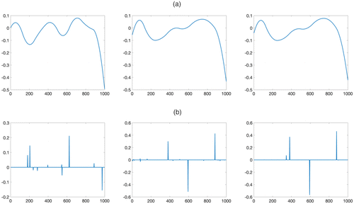
In the simulation study, we generate a 1D signal from and let . The smooth background is generated from a random linear combination of B-spline bases with three knots (i.e., , where and is a random vector such that , ). The incoherence condition parameter . The sparse signal component is generated by a sparse random linear combination of degree 2 B-spline bases with 500 knots : that is, , where and is a four-sparse random vector () such that its nonzero elements follow i.i.d. standard normal distribution. Notice that the RIC, for matrix , is hard to calculate in general. However, there is a loose upper bound that can be used, which is , where and are the maximum and minimum singular values of , respectively. The noise signal generated as a random vector is a random vector such that , . Figure 2 shows a sample raw signal and its smooth, sparse components.

Notes. (a) Raw signal. (b) Smooth signal component . (c) Sparse signal component .
Before we state the result, we first check the assumption of Theorems 2.3 and 2.4. For Theorem 2.3, it is easy to check that and also, that . For Theorem 2.4, , , and . Notice that the range for is small in this case because of the loose upper bound for , which can be further improved. This indicates that the smooth and sparse signal can be recovered by the proposed algorithm with high probability provided that the compressive ratio is above a specific threshold, which is demonstrated by the following observation.
The simulation is repeated 100 times, and the average log relative error for the background and sparse signal components with respect to compressive ratio are shown in Figure 3. We can observe a large error at the beginning, and it drops very fast with an increase of the compressive ratio. Then, above a threshold (0.1 approximately) of compressive ratio, the error becomes small (below 3%), and the decrease of error becomes less significant, which demonstrates the effectiveness of the reconstruction algorithm. The threshold of 0.1 can be chosen as the compressive ratio mentioned in Section 2.5.2.

Notes. (a) Log relative error for the smooth component. (b) Log relative error for the sparse component.
The reconstructed signal components in 1 of the 100 simulations are shown in Figure 4. We can observe that when adopting the compressive ratio of 0.1, both the smooth and sparse signal components can be reconstructed with high accuracy.
Notes. (a) Smooth signal component of compressive ratios 0.02 (left panel), 0.05 (center panel), and 0.1 (right panel). (b) Sparse signal component of compressive ratios 0.02 (left panel), 0.05 (center panel), and 0.1 (right panel).
We also vary the magnitude of sparse signals to examine the reconstruction performance of the proposed method. The result and analysis are provided in Appendix H.
3.2. CSSD on a 2D Image
In this simulation study, we aim to decompose an image into the smooth background, sparse anomalies, and noise. A image with smooth background and the sparse anomaly is generated similar to Yan et al. (2017) (i.e., , where is the smooth background, is the sparse anomalies, and is i.i.d. Gaussian noise such that ). The smooth background is generated from a linear combination of B-spline bases with knots, and the anomalies are generated from a sparse linear combination of B-spline bases with knots. The background and anomalies are shown in Figure 5.

We can see that the anomaly size covers a large range. The mean absolute value of the background plus anomaly is . In this simulation, we first study the reconstruction performance under a noise-free scenario. Then, we increase the noise level to test the robustness of the algorithm.
3.2.1. Noise-Free Case.
In this section, we vary the compressive ratio from 4% to 100%. For each compressive ratio, we simulate 100 times and the average false-negative rate (FNR) and false-positive rate (FPR) are reported in Figure 6. The FPR is defined as the portion of normal pixels predicted as anomaly,
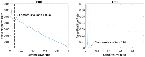
From Figure 6, we can see that both the FPR and FNR ratios decrease as the compressive ratio increases. The FPR drops so fast that when the compressive ratio achieves 8%, there is no false alarm, which is desired for the anomaly detection algorithm. The FNR drops slower, and less than 5% of the anomaly pixels are ignored when the compressive ratio achieves 8%. However, it does not miss any cluster of the anomalies, even though some of them are small.
The recovered sparse signal components are shown in Figure 7 for compressive ratios 4% (Figure 7(a)), 8% (Figure 7(b)), 33% (Figure 7(c)), and 73% (Figure 7(d)). For comparison, we apply the SSD algorithm (Yan et al. 2017), of which the FNR and the FPR are zero and computation time is 0.16 seconds.
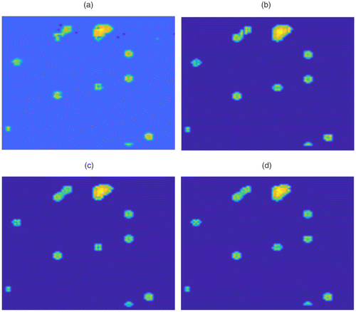
Notes. (a) Compressive ratio 4%. (b) Compressive ratio 8%. (c) Compressive ratio 33%. (d) Compressive ratio 73%.
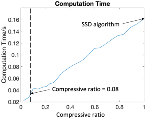
We record the computation time in Figure 8. A significant boosting of the computation is observed when the compressive ratio is 8%, which speeds up the SSD algorithm by 4.3 times.
3.2.2. Noisy Case.
The signal-to-noise ratio is studied to evaluate the robustness of the algorithm. The three-dimensional plot of FPR, the signal-to-noise ratio, and the compressive ratio are shown in Figure 9.
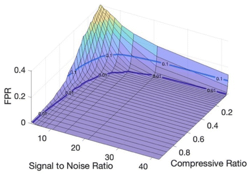
The purple line indicates the equipotential line of FPR = 0.01. We can see that with the increase of the signal-to-noise ratio, we are allowed to use a less compressive ratio to achieve satisfactory decomposition results. The majority of the area lies below the equipotential line of FPR = 0.01, which means that the proposed algorithm is robust.
4. Case Study
In this section, we use three real cases to demonstrate the effectiveness of the proposed CSSD/KronCSSD framework. For comparison, we also apply the SSD method in each case study. The compressive ratio () and the average computational time () for a single image are reported in Table 1. A significant transmission bandwidth reduction and computation boost can be observed with negligible performance degradation (Figures 10–12), compared with the vanilla SSD algorithm.
|

Table 1. Comparison Between KronCSSD and SSD
| Surface defect | Solar flare | Indentation | ||||
|---|---|---|---|---|---|---|
| /s | /s | /s | ||||
| KronCSSD | 54% | 0.073 | 22% | 0.034 | 48% | 0.053 |
| SSD | 1 | 0.135 | 1 | 0.086 | 1 | 0.094 |
Notes. (a) Raw image. (b) KronCSSD result. (c) SSD result.
Notes. (a) Raw image. (b) KronCSSD result. (c) SSD result.
Notes. (a) Raw image. (b) KronCSSD result. (c) SSD result.
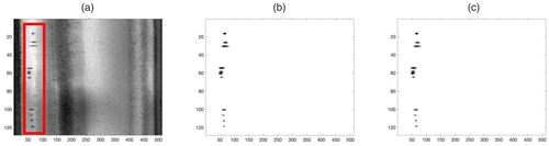
4.1. Surface Defect Detection in a Steel Rolling Process
As mentioned in Section 1, vision sensors collect high-resolution images of the product surface with a high data acquisition rate in the rolling processes. This poses a challenge in data storage, transmission, and processing. One sample image of size with typical anomalies is shown in Figure 10(a). The black scratches shown in the red block are surface anomalies. For a detailed description, the readers are encouraged to refer to Yan et al. (2018). The detected anomalies are shown in Figure 10, (b) and (c) by using the proposed KronCSSD algorithm and the SSD algorithm, respectively. The data set has 100 images, and more example results can be found in Appendix I.
The KronCSSD method achieves a similar anomaly detection performance with 54% bandwidth and is 1.8 times faster. By adopting the KronCSSD method, (i) we can achieve a faster anomaly detection and thus, reduce the loss through a timely intervention of the manufacturing process, and (ii) we can keep the manufacturing inspection information for a longer time period with the same storage capability, which is important for root cause analysis.
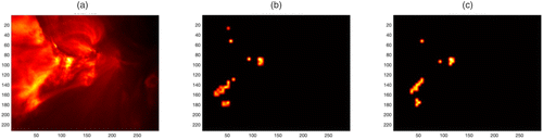
4.2. Solar Flare Detection
Another important application is solar flare detection from satellite images. A solar flare is defined as a sudden, transient, and intense variation in brightness over the sun’s surface. It has a significant influence on radio communication on Earth. Each second, thousands of high-resolution images are captured by a satellite, which poses a big challenge to real-time data transmission and processing (Yan et al. 2018). The data set has 300 images, and more example images can be found in Appendix I.
One sample image of size with a typical solar flare is shown in Figure 11(a), where the yellowish bright region is the solar flare. The detected anomalies are shown in Figure 11, (b) and (c) by using the proposed KronCSSD and SSD algorithms, respectively. The KronCSSD method achieves a similar solar flare detection performance as the SSD method but with 22% bandwidth, and it is 2.5 times faster. Notice that the decomposed images can also be used for downstream tasks, such as control charts and so on, which are beyond the scope of this paper.
By adopting the KronCSSD method, we can improve the transmission rate under the same transmission bandwidth and thus, achieve almost five times faster solar flare detection, which is of vital importance for protecting radio communications, power grids, and navigation systems.
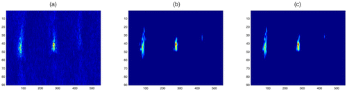
4.3. Silicon Surface Indentation Detection
The stress map of size of a silicon surface laminate with surface indentation is shown in Figure 12, where clusters of high-stress areas indicate the surface indentation (Yan et al. 2017). We aim to detect those high-stress areas. The detected anomalies are shown in Figure 12, (b) and (c). We can see that the KronCSSD method achieves a similar detection performance with the SSD method but with 40% bandwidth, and it is 1.8 times faster, which significantly reduces the storage and transmission cost and improves the processing speed.
5. Conclusion
In this paper, we proposed a CSSD framework for efficient data acquisition, transmission, and processing for sparse anomaly detection in smooth backgrounds. To further enhance its computational efficiency, a KronCSSD framework is proposed for tensor data.
The contributions of this work are twofold. (i) Theoretically, we showed the feasibility of combining compressive sensing and smooth sparse decomposition. This enables the adoption of a compressive data acquisition approach. (ii) Practically, the proposed framework is compatible with many existing decomposition-based anomaly detection algorithms, such as SSD, ST-SSD, and so on, which achieve both a significant cost reduction in sensing, storage, and transmission and a boost in speed but with negligible loss in their performance.
In this article, we use a simulation study to demonstrate the effectiveness and robustness of the proposed CSSD/KronCSSD framework. Three case studies across different applications demonstrate the versatility of the proposed framework. The authors believe that the CSSD/KronCSSD framework can be applied in a wider range of applications toward more efficient data acquisition, transmission, and processing.
Further studies on the theoretical properties of the proposed KronCSSD can be a future direction.
Appendix A
We prove Theorem 2.1 by contradiction. Assume there exists two different decompositions for the same smooth plus sparse signal (i.e., , where and ). Then,
Because , we can normalize both side by and denote and . Notice that is in the column space of , which is spanned by columns of the (recall that ; i.e., , where is the coefficient vector, ). Because , we have . We can bound each element in as follows:
According to Definition 2.1, and . Therefore, . Moreover, according to Equation (A.1), we conclude that . Denote the support of as ; we have , which is a contradiction. □
Appendix B
We prove Theorem 2.2 with contradiction. Assume there exists another vector such that and . Then, is a nonzero vector. Because , by Definition 2.3, we have that . Therefore, , which is a contradiction. Notice that the proof is inspired by the proof of lemma 3.1 in Candes and Tao (2005).
Appendix C
This proof is inspired by Baraniuk et al. (2008) and Tanner and Vary (2020).
We will first derive the RIC for a fixed subspace of when is restricted in a fixed subspace with the fixed support such that the number of nonzero elements is :
Then, we use a covering argument that counts over all possible sparse subspaces with support less than or equal to . Finally, we can derive the RIC for .
The following lemma describes the RIC for a fixed subspace and is proved in Appendix E.
RIC for a fixed subspace . Let be a matrix from the families described inDefinition 2.5. Furthermore, assume that and that the basis matrix for the sparse signal component satisfies the RIP with RIC : that is, is the smallest positive constant such that
For a given , there exists a constant depending only on , such that the RIC for is upper bounded by with the probability of at least , where , , , and .
Notice that for a fixed subspace , the RIP will fail with probability less than or equal to Because there are such subspaces, the probability to fail for , which is a combination of those subspaces, will be less than or equal to
Then, for any give , there exist , such that the probability to fail for is less than or equal to provided that where This finishes the proof.
Appendix D
The proof of Theorem 2.4 is inspired by Candes et al. (2006) and Tanner and Vary (2020). Assume that in Problem (1), is properly chosen such that Problem (1) is feasible. In the following discussion, we will use to denote the optimal solution of Problem (1) and to denote the signal we wish to recover. Let , where and are the residuals of the smooth and sparse signal components, respectively.
Let , where is the support of , denotes the projection of onto such that
Because is feasible and is the optimal solution of Problem (1), we must have which is equivalent to Because and are complementary to each other, we have Because , we have Hence, Because , we have
Similar to Candes et al. (2006), we order the elements of in decreasing order of their magnitude and enumerate as . Then, is divided into subsets of size , where
Let be the projection of onto ; we have
Define and , and combine Equations (D.1) and (D.2). Then, we have
Denote . (A tighter bound can be achieved by using . However, we adopt instead of for simplicity in the following proof.) Then, we have
Next, we derive the bounds for and .
Bound for
In the following discussion, we will bound those terms. According to the Cauchy–Schwarz inequality, the first term can be bounded as
The third term can be bounded as follows. Denoting and , we have
Therefore,
Similarly, the second term can be bounded as
Plugging Equations (D.5)–(D.7) into Equation (D.4), we have
According to the RIP property, we have
Consequently, we have
Bound for
In the following discussion, we will bound those terms. According to the Cauchy–Schwarz inequality, the first term can be bounded as
The third term can be bounded as follows. Denoting and we have
Therefore,
Plugging Equations (D.7), (D.11), and (D.12) into Equation (D.10), we have
According to the RIP property, we have
Consequently, we have
Notice that Equations (D.8) and (D.13) still hold if we relax to . For simplicity, here we replace with in the following derivation.
Plugging Equation (D.8) into Equation (D.13) and letting , we have
Here, we require in Equation (D.14) and let , which is
Let and c , where , , , and . If then there exist a such that Equation (D.15) is valid. Then, the denominator Consequently,
Notice that from Equations (D.1) and (D.9), we have
Therefore, where
Similarly, we can bound as where
Appendix E
In this section, we will provide the proof for Lemma C.1. By linearity of the measurement matrix , without loss of generality, it is enough to prove this lemma when . The proof mainly has two steps. First, the bounds for and are derived, and a finite set of points to approximate the set to any accuracy in norm 2 sense can be found. Then, the concentration inequality can be applied through a union bound. This is a common approach in compressive sensing literature (Baraniuk et al. 2008, Tanner and Vary 2020).
To derive the upper bounds for and , we first derive the upper bounds for the signals and , which are given in the following lemma.
The smooth signal component and sparse signal component of the signal in with can be bounded as follows:
The proof is presented in Appendix F.
According to the RIP for , we have
Combining Equations (E.2) and (E.3), we have
Denoting , we have Recall that ; we have where . Therefore, according to the triangle inequality and the Cauchy–Schwarz inequality, we have
Denoting , we have
Because we have derived the bounds for and , the covering number of is given by the following lemma whose proof is in Appendix G.
There exists a set , such that for all , with we have and , where is its cardinality.
Next, we will prove the main result by applying the concentration inequality (Definition 2.5(ii)) with union bound. Let ,
Because we have and . Then, Equation (E.4) can be written as
By the triangle inequality, we have
Define
Combining Equations (E.5) and (E.6), we have ; there exists a , such that with probability greater than .
Because , if , we have
If , we have
Notice that the second inequality comes from Equation (E.7) combined with being a covering of . In summary, we have
Because is attainable, according to Equation (E.7), we have Consequently, we have because . Therefore, with probability greater than .
Similarly, we can prove that with probability greater than .
Finally, according to Lemma E.2, we have that
This finishes the proof.
Appendix F
To prove the result, we first derive a nontrivial upper bound for the inner produce between and . Let be the reduced SVD of ; then,
Let because ; we have and
Therefore, we have
By completing the square, we have
Because , we have
Similarly, we can derive that
This finishes the proof.
Appendix G
We first state results for the covering number of a set (Vershynin 2018). The covering number of a smallest net for a unit norm ball in -dimensional space is .
Let and . There exist two finite covering sets of and , which are and .
For all and for all , we have
Therefore, we have and
Define . Then, , there exists a pair , such that
Therefore, is a covering of and This finishes the proof.
Appendix H. Simulation Study by Varying the Magnitude of Sparse Signals
We adopt the same simulation data generation procedure as in Section 3.1 while changing the distribution of elements in such that the nonzero elements follow i.i.d. normal distribution with mean zero and standard deviation in the range of . The example signals and reconstruction performance are shown in Figure H.1.
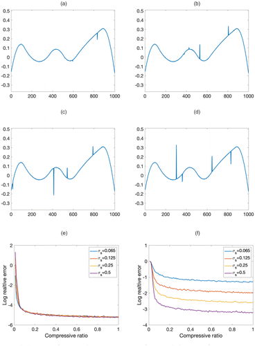
Notes. (a)–(d) Example signals corresponding to different , (e) log relative error for the smooth component, and (f) log relative error for the sparse component. (a) . (b) . (c) . (d) . (e) Log relative error for the smooth component. (f) Log relative error for the sparse component
There are several observations.
The log relative error of the smooth component does not change with different magnitudes of . This agrees with the theoretical result in Theorem 2.4, where the reconstruction error is bounded by a constant times the noise bound because the noise level is kept the same in all simulations.
The log relative error of the sparse component decreases as increases. This also agrees with the theoretical result in Theorem 2.4. Because the log relative error of the sparse component is defined as , according to Theorem 2.4, the reconstruction error term can be approximated by (i.e., , where is independent of ). increases as the magnitude of elements in increases. Therefore, will decrease as increases.
The 0.1 threshold (approximately) of the compressive ratio still holds with different magnitudes of sparse signal component.
Appendix I. Sample Case Study Images
Appendix I.1. Sample Images of Case Study 4.1
See Figure I.1.
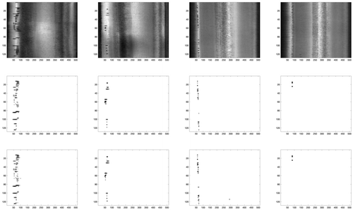
Notes. The top row shows raw images. The middle row shows corresponding SSD results. The bottom row shows KronCSSD results.
Appendix I.2. Sample Images of Case Study 4.2
See Figure I.2.
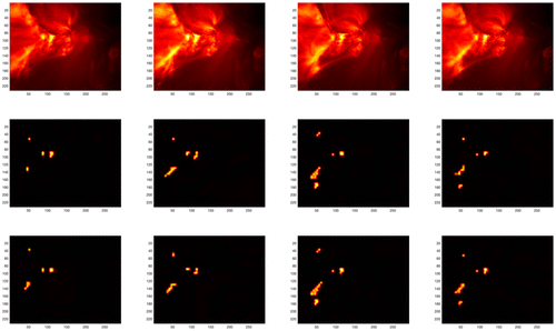
Notes. The top row shows raw images. The middle row shows corresponding SSD results. The bottom row shows KronCSSD results.
References
- (2011) Connection among spacecrafts and ground level observations of small solar transient events. Experiment. Astronomy 31(2):177–197.Google Scholar
- (2008) A simple proof of the restricted isometry property for random matrices. Constructive Approximation 28(3):253–263.Google Scholar
- (2014) Robust PCA via principal component pursuit: A review for a comparative evaluation in video surveillance. Comput. Vision Image Understanding 122:22–34.Google Scholar
- (2008) The restricted isometry property and its implications for compressed sensing. Competus Rendus Math. 346(9–10):589–592.Google Scholar
- (2005) Decoding by linear programming. IEEE Trans. Inform. Theory 51(12):4203–4215.Google Scholar
- (2006) Stable signal recovery from incomplete and inaccurate measurements. Comm. Pure Appl. Math. 59(8):1207–1223.Google Scholar
- (2011) Robust principal component analysis? J. ACM 58(3):1–37.Google Scholar
- (1978) A Practical Guide to Splines, vol. 27 (Springer-Verlag, New York).Google Scholar
- (2011) Kronecker compressive sensing. IEEE Trans. Image Processing 21(2):494–504.Google Scholar
- (1996) Flexible smoothing with B-splines and penalties. Statist. Sci. 11(2):89–121.Google Scholar
- (2011) USPACOR: Universal sparsity-controlling outlier rejection. Tichavsky P, Cernocky H, Prochazka A, eds. 2011 IEEE Internat. Conf. Acoustics Speech Signal Processing (IEEE, New York), 1952–1955.Google Scholar
- (2009) Tensor decompositions and applications. SIAM Rev. 51(3):455–500.Google Scholar
- (2013) Recovery of low-rank plus compressed sparse matrices with application to unveiling traffic anomalies. IEEE Trans. Inform. Theory 59(8):5186–5205.Google Scholar
- (2018) A review of sparse recovery algorithms. IEEE Access 7:1300–1322.Google Scholar
- (2011) Robust nonparametric regression by controlling sparsity. 2011 IEEE Internat. Conf. Acoustics Speech Signal Processing (ICASSP).Google Scholar
- (2015) Screen content image segmentation using sparse-smooth decomposition. 2015 49th Asilomar Conf. Signals Systems Comput.Google Scholar
- (2021) Additive tensor decomposition considering structural data information. IEEE Trans. Automation Sci. Engrg. 19(4):2904–2917.Google Scholar
- (2018) A systematic review of compressive sensing: Concepts, implementations and applications. IEEE Access 6:4875–4894.Google Scholar
- (2010) Guaranteed minimum-rank solutions of linear matrix equations via nuclear norm minimization. SIAM Rev. 52(3):471–501.Google Scholar
- (2020) Compressed sensing of low-rank plus sparse matrices. Preprint, submitted July 18, https://arxiv.org/abs/2007.09457v1.Google Scholar
- (1999) Splines: A perfect fit for signal and image processing. IEEE Signal Processing Magazine 16(6):22–38.Google Scholar
- (2018) High-Dimensional Probability: An Introduction with Applications in Data Science, vol. 47 (Cambridge University Press, Cambridge, United Kingdom).Google Scholar
- (2018) A spatial-adaptive sampling procedure for online monitoring of big data streams. J. Quality Tech. 50(4):329–343.Google Scholar
- (2011) SpaRCS: Recovering low-rank and sparse matrices from compressive measurements. Shawe-Taylor J, Zemel RS, Bartlett PL, Pereira F, Weinberger KQ, eds. Conf. Neural Inform. Processing Systems (Curran Associates Inc., Red Hook, NY), 1089–1097.Google Scholar
- (2012) Robust PCA via outlier pursuit. IEEE Trans. Inform. Theory 58(5):3047–3064.Google Scholar
- (2017) Anomaly detection in images with smooth background via smooth-sparse decomposition. Technometrics 59(1):102–114.Google Scholar
- (2018) Real-time monitoring of high-dimensional functional data streams via spatio-temporal smooth sparse decomposition. Technometrics 60(2):181–197.Google Scholar

