
The Value of Regulators as Monitors: Evidence from Banking
Abstract
While conventional wisdom suggests that financial supervision is costly for bank shareholders, agency theory suggests that supervisors’ audits can reduce shareholder monitoring costs. I study this trade-off in the context of an unexpected decrease in off-site surveillance intensity by the U.S. Federal Reserve. Banks subject to reduced surveillance experience a 1% loss in bank Tobin’s q and a 7% loss in equity market-to-book. These banks engage in more earnings management, and appear to compensate lower regulatory surveillance with costly internal audits. My results document a novel substitution effect between public monitoring by regulators and private monitoring by shareholders.
This paper was accepted by Victoria Ivashina, finance.
Supplemental Material: The online appendix and data files are available at https://doi.org/10.1287/mnsc.2021.03083.
1. Introduction
A widely-held view in the banking industry is that reporting to supervisory authorities has a negative impact on shareholder value: compliance subtracts resources from lending and deposit-taking activities, reduces profits, and ultimately hurts investors. This view gained momentum after the financial crisis due to an unprecedented increase in financial institutions’ reporting requirements (Arner et al. 2016), and regulatory bodies worldwide have been struggling to strike a balance between obtaining accurate data on supervised entities and limiting their regulatory burdens (e.g., FFIEC 2017).
While the current discussion highlights the costs of reporting for bank investors, banks are intrinsically opaque (e.g., Campbell and Kracaw 1980; Diamond 1989, 1991; Morgan 2002; Dang et al. 2017). Opacity can induce insiders to hide the bank’s true condition to shareholders, thus avoiding their interference (Leuz et al. 2003). By auditing banks’ information (Berger and Davies 1998, Flannery and Houston 1999, Berger et al. 2000), supervisors may align the incentives of bank shareholders and regulators, lift the burden of verification from shareholders, and increase bank value.
In this paper, I ask whether supervisory audits can benefit shareholders by reducing their private audit costs. I exploit an unexpected reduction in the reporting requirements of small U.S. Bank Holding Companies (BHCs) to the U.S. Federal Reserve (the Fed) as a quasi-exogenous source of variation in supervisory audit intensity, and I show that this change in reporting leads to large losses in the market value of affected banks.1 Consistent with a stylized model of costly state verification, I show that these losses are due to increased expenditures in internal controls systems and private audits—suggestive of an effort by bank outsiders to substitute supervision with private audits—, and to earnings management, suggestive of increased rent-seeking by bank insiders. I use various measures of bank complexity and opacity to show that value losses are larger when affected banks’ cash flows are more opaque.
Continuous off-site surveillance is a supervisory practice followed by most central banks worldwide, and one of the keystones of financial supervision in the United States (e.g., Barltrop and Sheng 1992, Sahajwala and Van Den Bergh 2000, Van Greuning and Brajovic Bratanovic 2009). Off-site surveillance consists of the collection, verification, and analysis of banks’ financial information to identify early warnings to banks’ safety and soundness. The timeliness and accuracy of banks’ reports are essential to remotely identify these early warnings, and supervisors devote significant resources in auditing banks’ financials and evaluating their internal reporting systems (see, e.g., Gilbert et al. 1999, Goldsmith-Pinkham et al. 2016). In sum, audits of banks’ financials are an essential component of off-site surveillance, and of supervision more in general (Flannery et al. 2004).
While supervisory audits are instrumental to off-site surveillance, identifying shocks to their intensity is challenging. Above all, these audits heavily rely on cross-bank comparisons, statistical analyses, and other automated procedures unobservable by the econometrician.2 In this paper, I exploit a change in the inputs to off-site supervisory audits—the financial reports that banks file with the regulator—to measure their impact on bank value. In early 2006, the Fed unexpectedly increased its minimum asset threshold for reporting requirements from $150 million to $500 million, providing reporting exemptions to around 1,300 privately-held BHCs and to 91 listed BHCs with assets between the old threshold and the new threshold (25% of all BHCs, and 5% of total BHC assets at the time). Using this reporting threshold change as a reduction in off-site audits for all small banks below $500 million in assets, I study changes in listed banks’ value around the new threshold in a difference-in-differences setting.
My identification strategy relies on the quasi-random assignment of treated banks just below the new threshold and control banks just above it before the Fed implemented the threshold change, such that systematic value differences after the change are arguably due only to the treatment. The quasi-random assignment assumption is supported by an institutional detail: smaller banks’ reporting exemptions were based on June 2005 BHC assets, but the threshold change was first announced by the Fed in November 2005, thus preventing banks’ strategic behavior around the new threshold.3
I find that, relative to control banks, banks treated with lower reporting requirements experience a 1% decrease in Tobin’s q and a 7% decrease in market-to-book ratios after the treatment. This finding is robust across a number of empirical specifications, sample restrictions, placebo tests, and falsification tests. For example, the treatment effect is stronger around the policy implementation date and threshold, and it disappears when I use placebo dates and thresholds to separate treated and control groups, ruling out sorting on size or differential exposure to aggregate trends as potential explanations for the main result. Moreover, the data shows no pre-existing value differences between treated and control banks, validating the common trends identifying assumption.
An event study reveals that the cumulative abnormal returns of treated banks experience large drops around the policy proposal and announcement dates relative to those of control banks, addressing timing concerns and concerns that the results might be due to changes in book values. I complement these results with a number of additional robustness tests. For example, I show that the results are not due to changes in disclosure, geographic clustering, differential exposure to local and aggregate economic conditions, and concurrent policies. Quantitatively, treated banks’ value losses are large, corresponding to a $4 million relative decrease in market capitalization for the average treated bank, and to an aggregate market capitalization loss of around $350 million.
How does this change in supervisory audits affect bank value and shareholders’ monitoring incentives from a theoretical standpoint? Using the lens of a costly state verification model, I build three testable predictions to guide the subsequent tests. In the model, a bank is comprised of a continuum of divisions. If a division is audited by the supervisor, bank shareholders need to pay a supervisory compliance cost but can observe the division’s true cash flow. If a division is not audited by the supervisor, shareholders need to set up a contract with the manager to incentivize truthful revelation of the division’s cash flows, and can privately arrange costly audits of the division (as in Townsend 1979, Gale and Hellwig 1985). The model shows that, if banks’ supervisory compliance costs are low enough, a reduction in the number of divisions audited by the supervisor leads to shareholder value losses. These losses are due to private audit expenditures and insider rents, and increase in cash flow opacity. Importantly, these predictions also hold on the intensive margin if the probability of a supervisory audit of any given cash flow decreases.
I provide three sets of empirical results consistent with these theoretical predictions. First, consistent with an increase in private monitoring incentives by treated banks’ shareholders, I document a 25% post-treatment increase in internal controls expenditure. Consistent with a negative cash flow effect, cross-sectional tests and mediation tests (Imai et al. 2010) show that treated banks’ value losses can partly be attributed to increased expenditure in internal monitoring.
Second, using a regression discontinuity design I confirm that banks just below $500 million in assets engage in more aggressive earnings management than banks just above $500 million in the years following the threshold change. I measure earnings management with bank discretionary loan loss provisions (LLPs)—the absolute negative residuals of a regression of LLPs on observables (e.g., Beatty and Liao 2014, Kanagaretnam et al. 2014). I show that banks below $500 million on average display 0.32% (one fourth of a standard deviation) lower discretionary LLPs than banks just above the threshold in the years following the treatment, and that these magnitudes are larger during the financial crisis and for public banks. I interpret these results as evidence of managerial rent extraction—an attempt by bank insiders to avoid intervention by concealing the firm’s true performance, especially in bad times (Healy and Wahlen 1999, Leuz et al. 2003, Jiang et al. 2016). Since bank-level data on LLPs is monitored by both the Fed and the regulators of bank subsidiaries, these results also confirm that audits by multiple regulators are useful on the intensive margin to reduce earnings management. Third, using supervisory complexity measures, measures of the materiality of the unmonitored business, and market-based measures of opacity, I show that that the baseline treatment effect is economically larger in treated banks whose cash flows are more opaque and difficult to evaluate by supervisors and market participants.
My results carry two policy implications. Regulators worldwide are considering decreasing their reliance on on-site inspections and increasing their reliance on off-site Supervisory Technology (“SupTech”) surveillance (Broeders and Prenio 2018).4 This paper suggests that off-site and on-site supervision have distinct roles in managing banks’ incentives, and that off-site surveillance may not be an effective substitute to on-site inspections to reduce bank risk-taking. Additionally, my results speak to a heated policy discussion on the costs and benefits of paperwork reduction policies for small and medium-sized banks in the United States. This paper shows that these reforms may miss their stated objective of reducing regulatory burden, and have private costs for bank shareholders.
This paper contributes to three strands of literature. The financial crisis has stimulated academic interest in the costs and benefits of financial regulation and supervision. This literature exploits variation in supervisory inspections and the closure of regulatory offices to show that on-site supervision improves bank efficiency and performance (Barth et al. 2013, Rezende and Wu 2014, Wilson and Veuger 2017), decreases bank risk-taking, leverage, and failures (Gopalan et al. 2017, Kandrac and Schlusche 2021), and has positive effects on lending allocation and the real economy (Agarwal et al. 2014, Granja and Leuz 2017, Passalacqua et al. 2021, Bonfim et al. 2022). I contribute to this literature by focusing on off-site surveillance, an essential but overlooked component of the supervisory process.5 I show that off-site surveillance can reduce insiders’ rent extraction, with large private benefits for bank shareholders. In other words, while the objectives of bank shareholders and regulators are generally different, the potential for rent extraction by insiders can align shareholders’ and regulators’ incentives. Different from the previous literature, I also show that off-site supervision may find a costly substitute in private audit arrangements.
Theoretical and empirical research shows that agency frictions are severe in banks. Bank assets are difficult to evaluate by outsiders and easy to modify by insiders: banks are opaque (Morgan 2002, Flannery et al. 2013, Dang et al. 2017), and opacity allows bank insiders to manage earnings and hide the firm’s true financial condition (Jiang et al. 2016). On-site inspections increase banks’ information quality (Berger and Davies 1998, Berger et al. 2000) and decrease banks’ intrinsic opacity (Flannery et al. 2004), with positive value effects (Flannery and Houston 1999). I contribute to this literature with a novel setting which allows me to separate audits from other activities performed by supervisors during on-site inspections, and by studying the incentives of insiders and outsiders following a reduction in audit intensity. I show that reporting and supervisory audits, which are aimed at facilitating off-site supervision, can generate private value for bank shareholders.
A long-standing question in financial economics is the extent to which monitoring affects shareholder value. Motivated by theoretical arguments (Shleifer and Vishny 1986, Kahn and Winton 1998, Maug 1998), the literature has focused on institutional ownership as a measure of monitoring to estimate the impact of monitoring on firm value (McConnell and Servaes 1990, Ferreira and Matos 2008). Causal inference is however difficult in these studies, because firm ownership and value are endogenously determined by firms’ contracting environment (Himmelberg et al. 1999, Coles et al. 2012). My paper contributes to this literature by using a novel identification strategy to estimate a large and positive impact of a specific type of monitoring—cash flow monitoring—on value. My results provide empirical support for the predictions of a traditional class of costly state verification models (Townsend 1979, Gale and Hellwig 1985), and are among the first to show that monitoring is valuable because it reduces earnings management incentives.6
2. Empirical Setting
2.1. Institutional Background and Framework
2.1.1. Off-Site Surveillance and Bank Reporting.
The Bank Holding Company Act of 1956 defines a BHC as any company that owns and/or has control over one or more banks. Commercial banks in the United States are not mandated to be part of a BHC. However, being part of a BHC offers substantial benefits, such as increased flexibility in raising external financing and acquiring other banks, as well as the ability to acquire nonbank subsidiaries. In practice, these benefits are such that at the end of 2016 around 84% of commercial banks in the United States were part of a BHC.7
The benefits of being part of a BHC come at the cost of compliance with the regulatory and supervisory requirements imposed by the Fed. From a regulatory standpoint, Regulation Y from 1980 gives the Fed exclusive authority in establishing BHC capital requirements, regulating BHC mergers and acquisitions, and defining and regulating nonbanking activities performed by BHC subsidiaries. From a supervisory standpoint, Section 5 of the Bank Holding Company Act provides guidance for the on-site and off-site inspections regularly conducted by regional Fed supervisors under delegated authority from the Board.
Supervisors conduct on-site inspections and continuous off-site surveillance to monitor the safety and soundness of BHCs. On-site inspections are the main supervisory tool of the Federal Reserve, and currently range from ad–hoc examinations for small BHCs to annual examinations and continuous on-site monitoring for the largest BHCs. During on-site inspections, supervisors assess the Risk Management (R), Financial Condition (F), and Impact (I) of BHC subsidiaries on other subsidiaries and on the holding company as a whole. These assessments result in a combined rating (RFI/C(D), previously known as BOPEC), which summarizes the overall condition of the consolidated BHC. Low RFI/C(D) ratings are serious warning signs for the BHC, and can result in corrective enforcement actions ranging from informal bank commitments and board resolutions to formal cease and desist orders and civil money penalties (see, e.g., Delis et al. 2016).
Since the early 1980s, on-site inspections are complemented by continuous off-site surveillance, which allows supervisors to remotely assess the financial condition of supervised BHCs in between on-site inspections. While off-site surveillance originally relied only on financial ratio analyses and supervisors’ judgment (Sahajwala and Van Den Bergh 2000), over the years supervisors adopted an increasingly data-oriented approach to identify early safety and soundness warnings using banks’ financial statements. As an example, the current U.S. off-site supervisory framework provides for the statistical analysis of hundreds of variables contained in banks’ financials (e.g., loans past due, loan loss provisions, capital ratios, off-balance sheet exposures) to produce watch lists, outlier lists, and Bank Holding Company Peer Reports (BHCPRs) aimed at identifying early warnings. Supervisors use the output of this remote surveillance process—such as surveillance screens and BHCPRs—to identify and delve into potential issues and to determine the scope and timing of on-site examinations.8
Due to its remote nature and heavy reliance on bank data, off-site surveillance hinges on the timeliness and accuracy of the reports that banks submit to the Fed. To this end, supervisors perform off-site audits and cross-firm analyses to ensure that the reported information is accurate. Supervisors can also request full and immediate access to internal audit reports and resources, and can take corrective actions if the bank’s internal audit systems are ineffective or if the reported information is deemed to be inaccurate. For example, Section 4080.1 of the BHC Supervision Manual states that “Surveillance information is crucial to identifying potential issues between reviews and for ensuring that on-site work is risk-focused. Accordingly, Reserve Banks are to continue taking steps to ensure the accuracy of the regulatory reports that are the basis for the surveillance program.” Goldsmith-Pinkham et al. (2016) show that supervisors’ interventions in banks’ audit and internal controls systems are indeed extremely common: In small and medium-sized BHCs, issues related to internal controls raise supervisory matters requiring attention (MRIs) more often than issues related to capital and liquidity.
In sum, supervisors follow an audit-like process aimed at reducing misrepresentations of the bank’s financial condition (e.g., Cole and Gunther 1998, Gilbert et al. 1999, Flannery et al. 2004). This audit process is arguably more intense than annual audits in public banks, as it is performed continuously; it uses additional data from multiple banks rather than data at the individual bank level to identify outliers and potential warnings; and it can lead to immediate on-site inspections and follow-up corrective actions with the board and the management. Additionally, supervisors are not hired by audited firms, which reduces the scope for collusion (see, e.g., Tepalagul and Lin 2015).
Banks’ financial reports are the main input to off-site financial supervision. Large BHCs need to file every quarter a consolidated financial statement (form FR Y-9C) and a holding parent company statement (form FR Y-9LP) containing detailed balance sheet, income statement, and off-balance sheet information about the BHC’s activity, as well as additional financial statements for the BHC’s nonbanking activities (forms FR Y-11). These financial statements, and form Y-9C in particular, are the main source of information for BHCs’ off-site surveillance. Additionally, Fed supervisors share, use, and monitor the information gathered by bank-level regulators in the quarterly Call Reports (forms FFIEC 031/041).9
To avoid regulatory burden, the Fed Board’s Small BHC Statement (Regulation Y, Appendix C) provides substantial reporting and supervisory exemptions to small banks. Small banks are exempted from filing form FR Y-9C, only file an annual statement for the parent company (form FR Y-9SP) with little consolidated information and substantially less information about the parent than the Y-9C and Y-9LP forms, and are exempted from filing form FR Y-11 for nonbank subsidiaries.10 While small BHCs’ bank subsidiaries still need to file the Call Reports, in Online Appendix A.1 I show that the Call Reports provide a partial and possibly distorted view of the BHC consolidated financials, and that these distortions increase with the size of the parent, the size of the nonbank activities and ownership complexity of the holding, and the size of the intra-BHC transactions. Finally, small BHCs are subject to simplified regulatory ratings, and fall out of the BHCPR analysis.11 In sum, just as they face lower on-site supervision (Goldsmith-Pinkham et al. 2016), small BHCs face lower reporting requirements and off-site supervision.
2.1.2. The 2006 Reporting Change.
Small and large BHCs are separated by a fixed asset size threshold. From 1986 until the end of 2005, the threshold was set to $150 million. In March 2006, the Fed implemented a regulation increasing the threshold to $500 million (71-FR-11194), providing new supervisory exemptions to all BHCs with assets between $150 million and $500 million.12 Figure 1 reveals that this regulation affected a large number of BHCs: more than 1,300 private BHCs and 91 listed BHCs (25% of all BHCs, and 5% of total BHC assets at the time) stopped filing their Y-9C consolidated financial statements and started filing the Y-9SP statement.
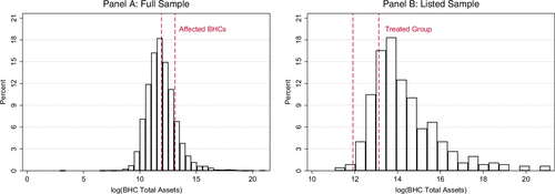
Notes. This figure shows the distribution of BHC (log) total assets in 2005, and highlights the sample of banks affected by the March 2006 reporting threshold change. Panel A shows the entire distribution of BHC total assets for both listed and unlisted BHCs, and highlights around 1,400 BHCs affected by the threshold change (those with 2005 assets between $150 million and $500 million). Panel B reports the distribution of listed BHCs and highlights the 91 listed BHCs in the treated group (around 20% of the listed BHCs in 2005).
In this paper, I exploit the 2006 change in small banks’ reporting requirements as a reduction in off-site supervision by the Fed for all banks below the $500 million threshold, and study value changes and shareholders’ monitoring incentives following this change. I argue that the 2006 threshold change reduced supervisory audits both on the extensive margin for the financial items reported in forms FR Y-9C, Y-LP, and Y-11, and on the intensive margin for the items contained in the Call Reports.
On the extensive margin, the consolidated BHC, the parent company, and the nonbank activities of the BHC were left unmonitored by the Fed. While one could argue that bank supervisors can use bank-level data to assess the consolidated condition of the BHC, Online Appendix A.1 shows that aggregated bank-level statements provide a partial and potentially distorted view of the consolidated performance of the holding company, even in relatively small BHCs such as the ones in my sample. On the intensive margin, the bank-level cash flows were left to be monitored by the bank regulator, reducing the overall probability of an audit.13
2.1.3. Theoretical Framework.
How does a change in supervisory audits’ intensity affect bank value and shareholders’ monitoring incentives from a theoretical standpoint? In Online Appendix A.2, I use the lens of a stylized model of costly state verification to provide a framework for the following empirical tests. In the model, a bank is comprised by a continuum of divisions. If a division is audited by the supervisor, bank shareholders need to pay a supervisory compliance cost but can perfectly observe the division’s true cash flow.14 If a division is not audited by the supervisor, shareholders need to set up a contract with the manager to incentivize truthful revelation of the division’s cash flows, and can privately arrange costly audits of the division. As in Townsend (1979) and Gale and Hellwig (1985), the optimal contract between bank shareholders and the manager trades off shareholders’ audit expenditures and managerial rents.
The main theoretical propositions of Appendix A.2 show that if banks’ supervisory compliance costs are low enough, a reduction in the number of divisions audited by the supervisor leads to shareholder value losses. These losses are due to increased private audit expenditures and insider rents, and an increasing function of cash flow opacity. I also show that these results hold on the intensive margin if the probability of a supervisory audit of any given cash flow decreases.
2.2. Data
The data on BHC total consolidated assets comes from the Federal Reserve Regulatory Data set. This data set is publicly available on the Federal Reserve of Chicago’s website, and it contains information sourced from the FR Y-9C, FR Y-9LP, and FR Y-9SP reports. I use the data set mainly to categorize BHCs into treated and control groups based on their 2005 average consolidated assets, and to keep track of which BHCs file which forms in each quarter.15 Since the Fed policy allows treated banks to stop reporting their FR Y-9C consolidated statements, I use Compustat Bank as the source of BHC consolidated financial data throughout the entire sample period. I combine this data set with CRSP to obtain end-of-quarter BHC Market-to-book values, and merge the Compustat-CRSP combined data set with the Federal Reserve Regulatory Data set using the link table available on the Federal Reserve of New York’s website.
The observation frequency is quarterly. The sample starts with the first quarter of 2004, and it ends with the last quarter of 2007. I focus on top-tier BHCs (defined as in Goetz et al. (2016) as BHCs that are not owned by any other BHC but possibly own other BHCs) with average 2005 total assets between $150 million and $850 million, and with stock price data available on CRSP. I assign individual BHCs to the treated group if their average total assets in 2005 are between $150 million and $500 million, and to the control group if their average total assets in 2005 are between $500 million and $850 million. I also impose the restriction that both treated and control BHCs are listed in 2005. The final estimation sample consists of 2,004 observations on 188 distinct BHCs (around 4% of the total number of BHCs in the United States at the end of 2005), out of which 91 belong to the treated group and 97 belong to the control group. In terms of size, these banks represent around 1% of the total assets in the banking sector at the end of 2005, and around 5% of the assets in the bottom 99% of the asset distribution. The average pre-treatment BHC asset size in my sample is $522 million, right above the policy implementation threshold.
Table 1 reports summary statistics for the main measures of bank value and internal monitoring expenditures, both in the full sample and in the treated and control subsamples. Table B2 in the Online Appendix reports additional summary statistics across treated and control groups.16 The first two rows of Panel A show summary statistics for the measures of bank value, Tobin’s q and the Market-to-book ratio of bank equity. The data shows little dispersion in these valuation ratios, both within the main sample and across the treated and control subsamples. The average and median Tobin’s q in the main sample are equal to 1.07 and 1.06, respectively, and the average and median Market-to-book ratios are 1.74 and 1.66, respectively.
|

Table 1. Summary Statistics
| Full Sample | Treated | Control | ||||||||||
|---|---|---|---|---|---|---|---|---|---|---|---|---|
| Mean | SD | Min | Med. | Max | N | Mean | SD | N | Mean | SD | N | |
| Panel A: Shareholder value and Professional fees | ||||||||||||
| Tobin’s q | 1.07 | 0.05 | 0.90 | 1.06 | 1.30 | 2,004 | 1.06 | 0.05 | 934 | 1.07 | 0.05 | 1,070 |
| Market-to-book | 1.74 | 0.54 | 0.41 | 1.66 | 4.24 | 2,004 | 1.68 | 0.53 | 934 | 1.79 | 0.54 | 1,070 |
| Professional fees | 0.22 | 0.16 | 0.00 | 0.17 | 1.11 | 941 | 0.17 | 0.14 | 500 | 0.27 | 0.16 | 441 |
| Panel B: Additional variables | ||||||||||||
| Leverage | 90.82 | 2.23 | 75.09 | 91.13 | 98.29 | 2,005 | 90.70 | 2.41 | 934 | 90.92 | 2.06 | 1,071 |
| Tier 1 ratio | 12.31 | 3.17 | 2.65 | 11.72 | 41.11 | 2,005 | 12.92 | 3.61 | 934 | 11.79 | 2.62 | 1,071 |
| Total assets | 571 | 234 | 114 | 548 | 1868 | 2,005 | 391 | 117 | 934 | 728 | 193 | 1,071 |
| Profitability | 22.31 | 36.41 | −839.33 | 25.98 | 226.26 | 2,005 | 18.26 | 51.18 | 934 | 25.83 | 13.09 | 1,071 |
| ROE | 2.33 | 2.91 | −63.79 | 2.60 | 20.82 | 2,005 | 1.92 | 3.94 | 934 | 2.68 | 1.44 | 1,071 |
| Diversification | 26.74 | 25.05 | −186.56 | 21.93 | 365.74 | 2,005 | 27.17 | 32.63 | 934 | 26.37 | 15.69 | 1,071 |
| Asset growth | 2.79 | 5.67 | −26.40 | 1.95 | 68.18 | 2,005 | 2.76 | 6.30 | 934 | 2.81 | 5.05 | 1,071 |
| Non-performing | 0.61 | 1.19 | 0.00 | 0.39 | 40.96 | 1,908 | 0.61 | 0.85 | 875 | 0.61 | 1.41 | 1,033 |
| Annual audit fees | 0.17 | 0.11 | 0.03 | 0.15 | 0.75 | 588 | 0.13 | 0.08 | 287 | 0.22 | 0.11 | 301 |
| Complexity | 2.31 | 1.26 | 2.00 | 2.00 | 9.00 | 1,783 | 2.21 | 1.12 | 909 | 2.42 | 1.38 | 874 |
Notes. This table reports summary statistics for the main variables used in the paper, both in the full sample and in the treated and control subsamples. In Panel A, Tobin’s q is the market value of total assets (market value of equity plus book value of debt) divided by the book value of total assets. Market-to-book is the market value of equity divided by the book value of equity. Professional fees are fees paid to consulting firms, investment banks, and auditing firms, in millions of US dollars. In Panel B, Leverage is total liabilities divided by total assets, the Tier 1 ratio is Tier 1 capital divided by risk-weighted assets, Profitability is net income divided by net interest income, ROE is net income divided by book value of equity, Diversification is noninterest income divided by net interest income, and Asset growth is quarterly growth in BHC Total assets. Non-performing assets are normalized by total assets. Annual audit fees come from Audit Analytics, and Complexity comes from form FR Y-9C in the last quarter of 2005. All the variables in Panel B except from Total assets (in USD millions), Annual audit fees (in USD millions), and Complexity (on a 2-9 scale) are reported in percentage terms. The sample used to construct the reported summary statistics is the estimation sample of Tables 2 and 5. The sample period for quarterly variables is 2004q1-2007q4. The sample period for Annual audit fees is 2004–2007.
The third row of Panel A shows summary statistics for bank Professional fees, in millions of U.S. dollars. These expenditures are recorded as separate items on the income statements that banks file with the Security Exchange Commission (SEC), and include fees paid to auditing, consulting, and investment banking firms. In the Online Appendix, I show that these expenditures are related to internal controls expenditure and audit fees in the sample of treated banks, suggesting an increased effort by outsiders to monitor insiders following the treatment. Panel A shows that banks in the treated group pay slightly lower Professional fees than banks in the control group. On average, treated banks spend 0.17 millions of dollars per quarter in Professional fees, with a standard deviation of 0.14 million. Control banks spend on average 0.27 millions of dollars per quarter, with a standard deviation of 0.16 million.
Panel B of Table 1 reports summary statistics for the other main variables in the paper. The variables in rows 1 to 8 are borrowed from the literature as potential determinants of cross-sectional heterogeneity in bank value (see, e.g., Laeven and Levine 2007, Minton et al. 2019), and include Leverage (total liabilities minus noncontrolling interest divided by total assets), the Tier 1 regulatory capital ratio (henceforth Tier 1 ratio, the bank self-reported ratio of Tier 1 capital divided by risk-weighted assets), Total assets, Profitability (net income divided by net interest income), return on equity (ROE, net income divided by book value of equity), Diversification (noninterest income divided by net interest income), quarterly Asset growth, and Non-performing assets (percentage non-performing assets to total assets).17 Row 9 of Panel B reports Annual audit fees from Audit Analytics, which I use to complement my main measure of private audits by outsiders (i.e., Professional fees). Row 10 reports pre-treatment BHC Complexity, corresponding to item BHCK9057 in form FR Y-9C in the last quarter of 2005. Overall, the data reveals little differences in these variables across treated and control groups, confirming the comparability of these two sets of banks.
2.3. Estimation Strategy and Identification
My empirical strategy compares the value of treated banks with pre-treatment total assets just below $500 million with the value of control banks with pre-treatment total assets just above $500 million, before and after the treatment. I estimate the model
The difference-in-differences empirical strategy relies on the identification assumption of quasi-random assignment of treated and control banks around the threshold before the Fed changes the reporting requirements of treated banks, such that any systematic value difference after the policy implementation is arguably due only to differences in Fed surveillance. This assumption can be violated for three reasons. First, the assumption is violated if the threshold change is lobbied (making the treatment an endogenous outcome) or otherwise anticipated by bank investors. Although the institutional details of the policy suggest that lobbying was unlikely—the policy was first proposed for public comment in November 2005, and the final policy was announced shortly after without modifications to the initial proposal—whether the policy was anticipated by shareholders is an empirical question.
In Figure 2, I report a diagnostic test aimed at detecting pre-existing differences in the average valuation of treated and control banks before the treatment. Panels A and B report these diagnostics for Tobin’s q and Market-to-book, respectively, and are constructed as follows. I first divide the sample into two subsamples, the pre-treatment sample ending with the last quarter of 2005 and the post-treatment sample starting with the first quarter of 2006. In each of these subsamples, I run a kernel-weighted local polynomial regression to obtain a smoothed estimate of the trend component of treated and control banks’ valuation. In Figure 2, I plot quarterly raw averages, these estimated trend components, and their associated confidence intervals as functions of the observation quarter, both in the pre- and post-treatment periods.
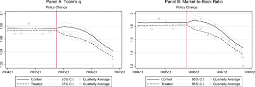
Notes. This figure reports a parallel trends diagnostic test on treated and control banks’ Tobin’s q (Panel A) and Market-to-book (Panel B). I first divide the sample into two subsamples, the pre-treatment sample ending in the last quarter of 2005 and the post-treatment sample starting in the first quarter of 2006. In each of these subsamples, I run a kernel-weighted local polynomial regression to obtain a smoothed estimate of the trend component of banks’ valuations. The local polynomial regression uses an Epanechnikov kernel and the rule-of-thumb bandwidth suggested in Fan and Gijbels (1996). The figure reports point estimates and 95% confidence intervals of the trend component of treated and control banks’ valuations as functions of the estimation quarter, as well as quarterly average Market-to-book and Tobin’s q. Tobin’s q and Market-to-book are defined as in Table 1.
Figure 2 shows that the trend components of treated and control banks’ valuation are statistically indistinguishable from each other in the pre-treatment period, supporting the claim that the threshold change was unanticipated. Moreover, the figure shows an increase in the difference between treated and control banks’ average valuation after the treatment, providing a visual preview of the results in the next section. Finally, the figure suggests that the increase in the difference between treated and control banks’ valuations is persistent and lasts until the end of my sample in 2007, a result that I formally confirm in the Online Appendix.19
Second, the identification assumption is violated if banks strategically adjust their size around the new threshold before its implementation. In Appendix Figure B3 (and its companion Appendix Table B3), I report the results of a McCrary (2008) discontinuity test aimed at addressing concerns of bank size adjustments around the $500 million threshold. I construct a finely-gridded histogram of bank Total assets, which I smooth on each size of the threshold using local linear regression. In Appendix Figure B3, I then plot point estimates and 95% confidence intervals of these smoothed asset densities during the 2005–2007 period (Panel A) and during the four quarters immediately before the treatment (Panel B). Both before and after the treatment, the estimated asset density below the threshold is not statistically different from the estimated asset density above the threshold. Additionally, an institutional feature of my quasi-natural experiment reduces residual concerns of asset manipulation before the treatment. The policy states that individual BHCs would qualify for reporting exemptions only if their June 2005 consolidated assets were below $500 million. At the same time, the Fed first publicly proposed the threshold change for public comment in November 2005, preventing pre-treatment size manipulation.
A third violation of the identification assumption arises from potential observable and unobservable differences across treated and control banks, which may differentially impact their valuations. Table 1 and several robustness tests in the paper and in the Online Appendix, however, suggest that treated and control banks do not systematically differ in terms of their observable characteristics nor in terms of their exposure to aggregate or local factors. For example, Figure 2 shows that such potential differences do not have value effects before the treatment. As another example, if such differences were simply the result of size or of changes in aggregate factors, the results would be economically weaker when restricting the sample bandwidth around the $500 million threshold (thus making treated and control banks even more comparable), and they would hold using arbitrary placebo size thresholds and treatment dates. In the robustness section below, I show that this is not the case. Overall, for the results to be driven by systematic differences across treated and control banks, these differences would have to be jointly systematically correlated with the specific size threshold of $500 million, and with the specific timing of the policy in early 2006, which seems unlikely.
3. Supervision and Bank Value
3.1. Main Result
Table 2 reports my main findings. The table reports point estimates for the coefficients in Equation (1), along with their standard errors (clustered at the BHC-level). The coefficient of interest is associated with the “Post × Treated” term, and represents an estimate of the percentage change in Tobin’s q and Market-to-book due to the treatment.
|
Table 2. Financial Supervision and Bank Shareholder Value
| log Tobin’s q | log Market-to-book | |||||
|---|---|---|---|---|---|---|
| (1) | (2) | (3) | (4) | (5) | (6) | |
| Post × Treated | −0.010*** | −0.011*** | −0.011*** | −0.074*** | −0.083*** | −0.079*** |
| (0.004) | (0.004) | (0.004) | (0.027) | (0.025) | (0.024) | |
| Leverage | 0.366*** | 0.301*** | 5.848*** | 5.596*** | ||
| (0.122) | (0.103) | (0.810) | (0.671) | |||
| Tier 1 Ratio | 0.395*** | 0.299*** | 2.671*** | 1.878*** | ||
| (0.080) | (0.072) | (0.524) | (0.493) | |||
| log Total Assets | −0.031*** | −0.223*** | ||||
| (0.008) | (0.049) | |||||
| Non-Performing Assets | −0.000 | −0.005 | ||||
| (0.001) | (0.007) | |||||
| Profitability | −0.005 | 0.024 | ||||
| (0.003) | (0.032) | |||||
| ROE | 0.104** | 0.619 | ||||
| (0.051) | (0.614) | |||||
| Diversification | −0.003 | −0.051 | ||||
| (0.005) | (0.034) | |||||
| Asset Growth | −0.010 | −0.059 | ||||
| (0.011) | (0.070) | |||||
| Year-quarter FE | Yes | Yes | Yes | Yes | Yes | Yes |
| BHC FE | Yes | Yes | Yes | Yes | Yes | Yes |
| R2 | 0.357 | 0.393 | 0.418 | 0.408 | 0.474 | 0.511 |
| Observations | 2,004 | 2,004 | 2,004 | 2,004 | 2,004 | 2,004 |
Notes. This table reports estimates of the treatment effect on bank value using the empirical specification in Equation (1). The coefficient associated with the “Post × Treated” interaction term captures the percentage change in treated bank value due to the treatment. The table includes year-quarter fixed effects (FE) and BHC FE. All the variables are defined as in Table 1. The sample period is 2004q1-2007q4. Standard errors (in parentheses) are clustered at the BHC-level.
***, **, and * respectively denote statistical significance at the 1%, 5%, and 10% levels.
When I estimate Equation (1) including only quarter- and BHC-level fixed effects, the treatment leads to a 1% decline in the Tobin’s q of treated banks, relative to the Tobin’s q of control banks. The economic magnitude and statistical significance of the coefficient are not affected by the inclusion of Leverage and the Tier 1 ratio to the specification, reducing concerns that the estimates might be driven by contemporaneous changes in small-bank capital requirements (see Appendix B.2.2). Everything else equal, a 10% increase in Leverage and Tier 1 ratios are respectively associated with a 3.4% and a 3.8% increase in Tobin’s q, but the treatment still induces a 1.1% decrease in Tobin’s q after the inclusion of these variables. Specification (3) shows that the results are also robust to the inclusion of assets, Profitability, Diversification, Asset growth, and Non-performing assets (a balance sheet proxy for bank risk) as additional controls.
In the last three specifications of Table 2, I repeat the same exercise using the natural logarithm of equity Market-to-book as a dependent variable. The treatment induces a 7.4% loss in Market-to-book for treated banks, and this value loss is as high as 8.3% when I add time-varying controls to the specification. To put these numbers in perspective, a 7% relative decrease in Market-to-book corresponds to a $4 million relative decrease in market capitalization for the average treated bank, implying an aggregate market capitalization loss of approximately $350 million. Finally, a comparison of the first three and the last three columns of Table 2 shows that the treatment effect on Tobin’s q is almost one order of magnitude smaller than the treatment effect on Market-to-book. This is due to leverage, which reduces the impact of equity fluctuations on the market value of bank assets.
3.2. Robustness
Table 3 reports two sets of tests aimed at reducing concerns about sample selection and possible violations of the identifying assumptions. In the interest of space, I present only the results for Market-to-book, leaving the results for Tobin’s q to Online Appendix Table B4. In Panel A, I test the impact of different sample bandwidth restrictions on the main result. In the first four specifications, I use two small samples of BHCs with average 2005 Total assets between $400 million and $600 million, and between $300 million and $700 million. In the last four specifications, I use two large samples of BHCs with Total assets between $150 million and $1 billion, and between $150 million and $1.5 billion. The table shows that the main results of the paper are not sensitive to different sample bandwidth choices. Moreover, the first four specifications show that the treatment leads to larger value drops for BHCs closer to the threshold. Since the results are statistically identical and economically larger when I restrict the sample to relatively comparable banks around the $500 million threshold, Panel A confirms that my results are not just a simple reflection of size differences across treated and control banks.
|
Table 3. Robustness and Placebo Tests: Market-to-Book
| Panel A: Sample bandwidth selection | ||||||||
|---|---|---|---|---|---|---|---|---|
| $400M-600M | $300M-700M | $150M-1B | $150M-1.5B | |||||
| (1) | (2) | (3) | (4) | (5) | (6) | (7) | (8) | |
| Post × Treated | −0.103** | −0.122*** | −0.079** | −0.090*** | −0.068*** | −0.080*** | −0.063*** | −0.075*** |
| (0.04) | (0.03) | (0.03) | (0.03) | (0.02) | (0.02) | (0.02) | (0.02) | |
| Linear distance pol. | Yes | Yes | Yes | Yes | Yes | Yes | Yes | Yes |
| Other controls | No | Yes | No | Yes | No | Yes | No | Yes |
| Year-quarter FE | Yes | Yes | Yes | Yes | Yes | Yes | Yes | Yes |
| BHC FE | Yes | Yes | Yes | Yes | Yes | Yes | Yes | Yes |
| R2 | 0.464 | 0.573 | 0.452 | 0.561 | 0.455 | 0.525 | 0.477 | 0.534 |
| Observations | 650 | 650 | 1,324 | 1,324 | 2,372 | 2,372 | 2,922 | 2,922 |
| Panel B: Placebo tests | ||||||||||
|---|---|---|---|---|---|---|---|---|---|---|
| $300M | $750M | $1B | 12/2004 | 12/2006 | ||||||
| (1) | (2) | (3) | (4) | (5) | (6) | (7) | (8) | (9) | (10) | |
| Post × Treated | −0.034 | −0.002 | 0.011 | −0.001 | 0.035 | −0.008 | −0.001 | 0.025 | 0.005 | 0.022 |
| (0.04) | (0.04) | (0.03) | (0.03) | (0.03) | (0.03) | (0.03) | (0.03) | (0.03) | (0.02) | |
| Controls | No | Yes | No | Yes | No | Yes | No | Yes | No | Yes |
| Year-quarter FE | Yes | Yes | Yes | Yes | Yes | Yes | Yes | Yes | Yes | Yes |
| BHC FE | Yes | Yes | Yes | Yes | Yes | Yes | Yes | Yes | Yes | Yes |
| R2 | 0.423 | 0.553 | 0.394 | 0.545 | 0.427 | 0.558 | 0.036 | 0.157 | 0.556 | 0.672 |
| Observations | 934 | 934 | 1,438 | 1,438 | 1,988 | 1,988 | 964 | 964 | 1,040 | 1,040 |
Notes. This table reports sample bandwidth selection tests (Panel A) and placebo tests (Panel B) on the main Market-to-book result from Table 2. In Panel A, I use two small samples of BHCs with average 2005 Total assets between $400 and $600 million (columns (1)-(2)), and between $300 and $700 million (columns (3)-(4)). In the last four specifications, I use two large samples of BHCs with Total assets between $150 million and $1 billion, and between $150 million and $1.5 billion. To control for potential differences in the size-valuation relationship as the sample changes, the regressions in Panel A include linear polynomials in bank size above and below the threshold. In Panel B, columns (1) and (2), I use a placebo asset threshold of $300 million and a symmetric sample of [$150, $500] million around this threshold to define treated and control placebo groups. In columns (2)-(3) and (3)-(4), I respectively use placebo thresholds of $750 million (with a symmetric sample of [$500, $1000] million) and $1 billion (with a symmetric sample of [$0.5, $1.5] billion) in Total assets. The sample period is 2004q1-2007q4. In specifications (7) and (8), I use the last quarter of 2004 as the placebo treatment quarter, dropping post-2005 observations from the sample. In the last two specifications, I use the last quarter of 2006 as the placebo treatment quarter, dropping pre-2006 observations from the sample. The sample in these two columns is otherwise the same as the sample in Table 2. The dependent variable in all specifications is the natural logarithm of bank Market-to-book, and the unreported control variables are the same as in Panel A. Standard errors (in parentheses) are clustered at the BHC-level.
***, **, and * respectively denote statistical significance at the 1%, 5%, and 10% levels.
In Panel B, I show that the statistical significance and the economic magnitude of the results disappear when I separate treated and control banks using arbitrary treatment thresholds and quarters. The first six specifications show that the results disappear when I use placebo asset thresholds of $300 million, $750 million, and $1 billion to separate treated and control banks, further addressing concerns that the effects documented in Table 2 might be due to systematic differences between treated and control banks correlated with size. Similarly, the last four specifications show that the results disappear when I use the last quarter of 2004 and the last quarter of 2006 as placebo treatment quarters. Overall, Tables 3 and B4 confirm that my main results are specific to both the specific $500 million asset threshold and the specific timing of the policy, providing support for the identifying assumptions.
A second concern is that the main result might be due to an increase in treated banks’ book value of equity, and that quarterly measurement of the dependent variable may induce confounding variation in market equity values. Table 4 and Appendix Table B5 provide evidence from event studies around the announcement date of the policy proposal 70-FR-66423 (November 2, 2005) and that of the final policy 71-FR-11194 (March 6, 2006) aimed at addressing such concerns. In Table 4, I first compute treated banks’ Buy-and-Hold Abnormal Returns (BHARs) benchmarked against equally-weighted portfolios of control banks’ stocks. These Buy-and-Hold Abnormal Returns are constructed as average differences between treated banks’ individual cumulative returns in the event window, and the cumulative returns of the benchmark portfolio of control banks (see, e.g., Kothari and Warner 2007), thus allowing me to compare relative return differences in two sets of similar banks while retaining the statistical power of the full treated sample.
|
Table 4. Event Study
| Full sample | 2005 announcement | 2006 announcement | |||||||
|---|---|---|---|---|---|---|---|---|---|
| BHAR(%) | t-stat | N | BHAR(%) | t-stat | N | BHAR(%) | t-stat | N | |
| −1 to 1 | −0.372 | −2.040 | 168 | −0.469 | −1.525 | 83 | −0.278 | −1.348 | 85 |
| −3 to 3 | −0.640 | −2.716 | 168 | −1.192 | −3.453 | 83 | −0.101 | −0.314 | 85 |
| −5 to 5 | −0.593 | −2.313 | 168 | −0.752 | −1.875 | 83 | −0.437 | −1.344 | 85 |
| −7 to 7 | −1.258 | −4.714 | 168 | −1.408 | −3.723 | 83 | −1.111 | −2.936 | 85 |
| −10 to 10 | −1.115 | −3.344 | 168 | −0.956 | −1.788 | 83 | −1.269 | −3.231 | 85 |
| −15 to 15 | −2.329 | −4.902 | 168 | −1.457 | −1.995 | 83 | −3.181 | −5.981 | 85 |
Notes. In this table, I report the results of an event study around the announcement date of the policy proposal (November 2, 2005) and around the announcement date of the final policy (March 6, 2006). I first compute treated banks’ Buy-and-Hold Abnormal Returns (BHARs) benchmarked against equally-weighted portfolios of control banks’ stocks. In the table, I report average BHARs and their associated skewness-adjusted bootstrapped t-statistics (Lyon et al. 1999) for windows of [−1,1] to [−15,15] days around the event. In the first three columns of the table, I report the full-sample results with multiple bank-level observations. In the third to sixth columns, I report results around the announcement date of the policy proposal (November 2, 2005), and in the last three columns I report results around the announcement date of the final policy (March 6, 2006).
In the first three columns of Table 4, I report average BHARs and their associated skewness-adjusted bootstrapped t-statistics (Lyon et al. 1999) for windows of [−1, 1] to [−15, 15] days around the event in the full sample which includes multiple bank-level observations. This panel shows that, around each event, treated banks experience negative average BHARs of up to −2.33% relative to the benchmark equally-weighted portfolio of control banks. The difference between the average treated stock’s cumulative returns and the control stock’s portfolio cumulative return around the event date is statistically significant at conventional levels, with t-statistics in excess of 2 even in a narrow window of [−1, 1] days around the event dates. Quantitatively, these average estimates translate into a total relative decrease in market value of around 4.7%, a magnitude comparable to the main effect documented in the difference-in-differences test.
In the last six columns of the table, I separately report estimated BHARs around the announcement date of the policy proposal (November 2, 2005) and around the announcement date of the final policy (March 6, 2006). These two panels reveal an economically small but statistically significant effect around the proposal announcement date, and an economically larger effect around the final policy announcement date, perhaps due to investors’ uncertainty about the final policy, or to its salience once banks stop filing their statements with the Fed.
In Appendix Table B5, I conduct additional robustness on the event study using different BHAR estimation windows. Table B5 shows no evidence of negative BHARs for windows of up to 10 trading days from the announcement of either the proposed policy or the final policy, and large negative BHARs just-around the proposed policy announcement on November 2, 2005. The table also shows relatively large negative BHARs between 10 and 5 days from the final policy announcement date on March 6, 2006, suggesting that the final passage of a contemporaneous policy on small-bank capital requirements may have changed investors’ expectations about small banks’ reporting requirements.20 Online Appendix Figure B4 also reports the results of Table B5 in graphical form. Overall, the results of Table 4, Table B5, and Figure B4 confirm large losses in treated banks’ market capitalization around the policy announcement dates.
Online Appendix B.1.1 also contains the results of ten additional robustness tests, including alternative sample restrictions, variable definitions, and robustness to aggregate and local economic variation. Overall, the tests contained in this section and in the Online Appendix provide support for the robustness of my main finding, as well as for a causal interpretation.
4. Mechanism
The value losses documented in the previous section show that the benefits of supervisory audits can exceed the costs of reporting and supervision. In this section, I use the lens of the costly state verification model to provide additional supporting evidence for this proposed mechanism.
4.1. Private Audits and Internal Controls
I first argue that part of the post-treatment value losses of treated banks are due to increased private monitoring expenditure. In Table 5, I start by documenting a large treatment effect on treated banks’ quarterly Professional fees, which include quarterly expenditures for audits and internal controls.21 Table 5 reports a large, 25% post-treatment increase in treated banks’ quarterly Professional fees starting from the first quarter of 2006. This difference is economically large, amounting to approximately 43,000 dollars per quarter on average. When I discount 43,000 dollars of increased expenditures (after-taxes) at an average quarterly discount rate of 2% in perpetuity, their discounted present value amounts to slightly less than 1.5 million dollars, around 38% percent of the 4 million (relative) market value drop experienced by the average treated bank. In other words, increased Professional fees quantitatively correspond to a large fraction of the average value loss experienced by treated banks.
|
Table 5. Private Audits: Quarterly Professional Fees
| log Professional fees | log | |||||
|---|---|---|---|---|---|---|
| (1) | (2) | (3) | (4) | (5) | (6) | |
| Post × Treated | 0.243** | 0.254*** | 0.224*** | 0.210** | 0.212** | 0.213*** |
| (0.09) | (0.09) | (0.07) | (0.09) | (0.09) | (0.07) | |
| Leverage | −1.681 | −1.552 | 2.492 | 0.703 | ||
| (3.30) | (2.52) | (3.14) | (2.51) | |||
| Tier 1 Ratio | −4.525*** | −2.124 | −1.519 | −1.273 | ||
| (1.55) | (1.33) | (1.49) | (1.32) | |||
| Other controls | No | No | Yes | No | No | Yes |
| Year-quarter FE | Yes | Yes | Yes | Yes | Yes | Yes |
| BHC FE | Yes | Yes | Yes | Yes | Yes | Yes |
| R2 | 0.070 | 0.099 | 0.194 | 0.046 | 0.065 | 0.152 |
| Observations | 941 | 941 | 941 | 941 | 941 | 941 |
Notes. This table documents an increase in treated banks’ quarterly Professional fees following the treatment. In the first three specifications of this table, I use the natural logarithm of Professional fees as a dependent variable, and in the last three specifications I use the natural logarithm of Professional fees normalized by Net interest income. Additional control variables not reported in the table include Profitability, Total assets, ROE, Diversification, Asset growth, and Non-performing assets. Standard errors (in parentheses) are clustered at the BHC-level.
***, **, and * respectively denote statistical significance at the 1%, 5%, and 10% levels.
Next, I link treated banks’ value losses to Professional fees. In Appendix Table B23, I first divide treated and control banks into two groups based on whether, after the treatment, they incur above- or below-median Professional fees relative to their Net interest income. Then, I run a triple differences specification including a “Post × Treated × High Professional fees” term to capture value changes for treated banks that pay relatively high Professional fees per dollar of income after the treatment. The table shows that the treatment effect is concentrated in the subsample of treated banks with high post-treatment Professional fees, supporting the hypothesis that the value losses experienced by treated banks are partially due to a cash flow effect from increased Professional fees.22
In Appendix Table B24, I complement the analysis of Table B23 with a mediation test (see, e.g., Imai et al. 2010) aimed at quantifying the extent to which the drop in treated banks’ market to book arises from internal monitoring expenditures. I first orthogonalize log Professional fees and log Market-to-book with respect to year-quarter and BHC fixed effects to remove bank- and time-specific average differences in valuations and Professional fees. In Panel A of Table B24, I report the results of a first-stage regression of (log) Professional fees on the “Post × Treated” indicator, and of a second-stage regression of (log) Market-to-book on the “Post × Treated” indicator and on log-Professional fees. In Panel B, I report the results of the mediation analysis, which shows that around 11% of the total treatment effect on bank value comes from an increase in Professional fees. The relatively small magnitude of the mediated effect may be due to stock prices reflecting the discounted present value of the entire stream of treated banks’ future Professional fees, and to revised shareholder expectations about future earnings management.
4.2. Earnings Management
In this section, I employ an RD design around the new $500 million threshold to document an increase in treated banks’ earnings management after the treatment.23 Following the bank accounting literature (see, e.g., Beatty and Liao 2014 for a review), I use discretionary LLPs as my main measure of earnings management, and study changes in discretionary LLPs for BHCs with total assets just above and just below $500 million after 2006.
I first construct bank-level Discretionary LLPs as the absolute negative residuals of a first-stage regression of LLPs (as a percentage of total loans) on lagged loan loss allowances, contemporaneous loan charge-offs to assets, loans to assets, non-performing loans to assets, changes in total loans scaled by total assets, and firm fixed effects (Kanagaretnam et al. 2014). Appendix Table B25 provides summary statistics for the variables used in this section. I link these bank-level discretionary negative LLPs to the total assets of their top-holding BHC, and study differences in Discretionary LLPs around the $500 million threshold using a local linear regression estimator of the form
The first column of Table 6, Panel A, reports the estimate of coefficient β2 in Equation (2). This column shows that banks whose top-holder BHC’s assets are just above $500 million have around 0.32% lower discretionary negative LLPs than banks just below this threshold. This effect is large, amounting to around one-fourth of a standard deviation in Discretionary LLPs in the sample. In columns (2) and (3), I augment the baseline specification (1) with second- and third-order polynomials in BHC size to control for possible nonlinearities in the relationship between Discretionary LLPs and size around $500 million. The economic magnitude of the estimates is even larger in these specifications, and the estimates’ statistical significance is not affected by the inclusion of the size polynomials. In Appendix Figure B6, I visually confirm the results of the first three columns of Panel A by documenting a discontinuity in Discretionary LLPs in a narrow window around the $500 million threshold.
|
Table 6. Regression Discontinuity: Post-Treatment Earnings Management
| All banks | Public banks | |||||
|---|---|---|---|---|---|---|
| (1) | (2) | (3) | (4) | (5) | (6) | |
| Panel A: Full sample | ||||||
| RD estimate | −0.324*** | −0.391*** | −0.429*** | −2.335*** | −2.639*** | −2.724*** |
| (0.09) | (0.12) | (0.12) | (0.62) | (0.69) | (0.73) | |
| Polynomial order | 1 | 2 | 3 | 1 | 2 | 3 |
| Kernel type | Triangular | Triangular | Triangular | Triangular | Triangular | Triangular |
| Observations | 37,770 | 37,770 | 37,770 | 1,737 | 1,737 | 1,737 |
| Panel B: Financial crisis | ||||||
| RD estimate | −0.683*** | −0.713*** | −0.902*** | −2.727*** | −3.285*** | −3.541*** |
| (0.14) | (0.16) | (0.21) | (0.74) | (0.84) | (0.91) | |
| Polynomial order | 1 | 2 | 3 | 1 | 2 | 3 |
| Kernel yype | Triangular | Triangular | Triangular | Triangular | Triangular | Triangular |
| Observations | 14,789 | 14,789 | 14,789 | 699 | 699 | 699 |
Notes. This table presents the results of a regression discontinuity design (RDD) to detect changes in Discretionary LLPs around the $500 million supervisory cutoff after the treatment and during the financial crisis. The RDD relies on polynomials of order 1 to 3 and a triangular kernel, with bandwidth chosen via the mean squared error optimal bandwidth approach proposed in Calonico et al. (2014). Using the FDIC call reports, I construct bank-level Discretionary LLPs as the absolute negative residuals of a first-stage regression of loan loss provisions (normalized by total loans) on lagged loan loss allowances, contemporaneous loan charge-offs to assets, loans to assets, non-performing loans to assets, changes in total loans, and charter fixed effects (Kanagaretnam et al. 2014). I then link these bank-level absolute negative residuals to BHC-level Total assets. The table reports estimates of the mean predicted difference in Discretionary LLPs for firms just below and just above the $500 million supervisory threshold, both unconditionally and during the crisis. The sample period in Panel A is 2006q1-2014q4. The sample period in Panel B is 2008q1-2010q4. Similar to the main tests, the sample includes the universe of banks that are part of a BHC with assets between $150 and $850 million. Calonico et al. (2014) robust bias-corrected standard errors in parentheses.
***, **, and * respectively denote statistical significance at the 1%, 5%, and 10% levels.
One of the main advantages of bank-level abnormal LLPs as a measure of earnings management (above and beyond their widespread use, Beatty and Liao 2014) is that abnormal LLPs are available for both private and public banks, which allows me to study earnings management in BHCs with different sets of incentives. Public banks face opposing incentives to engage in earnings management—while reporting to the SEC may decrease public firms’ earnings management incentives, public ownership and short-term targeting may exacerbate these incentives (Beatty et al. 2002). As a result, it is ex-ante not clear whether one should expect higher or lower provisioning in public banks. The results of columns (4) to (6) of Panel A show that the baseline effects of supervision on discretionary provisioning are around six times larger when banks belong to a publicly-listed BHC, suggesting that public filing does not compensate increased earnings management incentives induced by public ownership.25
An RDD over a longer sample period also allows me to study earnings management incentives over the business cycle. Using the financial crisis as a laboratory, in Panel B of Table 6 I confirm that treated banks’ incentives to overstate earnings are more pronounced in bad times. Since Discretionary LLPs are orthogonalized with respect to bank-level time-varying characteristics, the results of Panel B are reflective of increased earnings management incentives during the crisis as opposed to changes in bank performance during the period. Panel B shows that the baseline effects of Panel A approximately double in magnitude during the financial crisis, both in the full sample and in the sample of publicly-listed banks.
In Online Appendix Section B.1.3, I provide additional robustness on the results of Table 6, as well as additional evidence using alternative measures of earnings management. Overall, Table 6 and the results contained in this Online Appendix confirm off-site surveillance as an effective tool to reduce earnings management, especially when earnings management incentives are stronger in the time series and in the cross-section. Consistent with my theoretical framework, Table 6 also suggests that the 2006 experiment leads to a decrease in the probability of regulatory audits for bank-level cash flows, even if these cash flows are also audited by the regulators of the bank subsidiary.26 In other words, Table 6 suggests that off-site supervision by multiple regulators increases the probability of an audit by any of these regulators, and that this reduces managerial earnings management incentives. These results complement those in Agarwal et al. (2014) by showing that, by increasing the probability of an audit, monitoring by multiple regulators can improve bank outcomes. Table 6 also shows that the main proposition of this paper—that supervision reduces bank earnings management incentives and increases information quality—holds more generally than in the specific environment of the 2006 experiment.
4.3. Evidence from Opaque Banks
In this section, I go back to the main 2006 experiment and test the theoretical prediction that treated banks whose cash flows are more opaque and hence difficult to evaluate by outsiders should experience larger post-treatment value losses. I use two sets of opacity measures to verify this hypothesis, one based on supervisors’ assessments of the complexity of the BHC, and one based on market participants’ assessments of the opacity of the BHC. My results are consistent across these two sets of measures.
4.3.1. Supervisory Complexity.
In Table 7, I run triple-differences specifications to study differential treatment effects on banks with high supervisory complexity ratings. Supervisory complexity has two benefits as a measure of opacity. First, Fed supervisors assess complexity based on their off-site readings of a BHC’s financials, which allows me to measure opacity from the perspective of (off-site) supervisors as opposed to other bank outsiders. Second, the four sources of accounting discrepancy between the BHC-level financials and the bank-level financials highlighted in Appendix A.1 are included as criteria to determine BHC complexity, which also allows me to use complexity as a catch-all proxy for the materiality of the unmonitored business.27
|
Table 7. Cross-Sectional Evidence: Supervisory Complexity
| Complexity | Complexity determinants | |||||||
|---|---|---|---|---|---|---|---|---|
| (1) | (2) | (3) | (4) | (5) | (6) | (7) | (8) | |
| Post × Treated | −0.060** | −0.061** | −0.060** | −0.050 | −0.072*** | −0.105*** | −0.066* | −0.086** |
| (0.03) | (0.03) | (0.03) | (0.03) | (0.03) | (0.04) | (0.04) | (0.04) | |
| Post × Treated × Complex | −0.208** | |||||||
| (0.09) | ||||||||
| Post × Treated × Uns. Complex | −0.235*** | |||||||
| (0.04) | ||||||||
| Post × Treated × High Min. Inv. | −0.215** | |||||||
| (0.10) | ||||||||
| Post × Treated × High NB Assets | −0.056 | |||||||
| (0.05) | ||||||||
| Post × Treated × High Bank Subs. | 0.025 | |||||||
| (0.10) | ||||||||
| Post × Treated × High P. Assets | 0.072 | |||||||
| (0.05) | ||||||||
| Post × Treated × High Leverage | −0.007 | |||||||
| (0.05) | ||||||||
| Post × Treated × Shell | 0.025 | |||||||
| (0.05) | ||||||||
| Low-order terms | Yes | Yes | Yes | Yes | Yes | Yes | Yes | Yes |
| Controls | Yes | Yes | Yes | Yes | Yes | Yes | Yes | Yes |
| Year-quarter FE | Yes | Yes | Yes | Yes | Yes | Yes | Yes | Yes |
| BHC FE | Yes | Yes | Yes | Yes | Yes | Yes | Yes | Yes |
| R2 | 0.514 | 0.506 | 0.512 | 0.512 | 0.508 | 0.511 | 0.508 | 0.510 |
| Observations | 1,783 | 1,697 | 1,783 | 1,783 | 1,783 | 1,783 | 1,783 | 1,783 |
Notes. In this table, I run a triple-differences specification to study differential treatment effects on banks with different levels of opacity, using BHC complexity as a measure of opacity from the perspective of the supervisor. In column (1), I interact the baseline “Post × Treated” treatment effect indicator with an indicator equal to one if pre-treatment BHC Complexity is above median, and equal to zero otherwise. In column (2), I repeat the same exercise using an indicator equal to one if the BHC is complex but not supervised (corresponding to a complexity rating of 9), and equal to zero if the BHC is not complex. In the remainder of the table, I study specific determinants of Complexity by interacting the treatment effect indicator with indicators for above-median pre-treatment minority investments to total assets (column (3)), nonbanking assets to total assets (column (4)), bank subsidiaries (column (5)), parent assets to total assets (column (6)), and leverage (column (7)), and for whether the BHC is a one-bank shell before the treatment (column (8)). The unreported control variables are the same as in Table 2. Standard errors (in parentheses) are clustered at the BHC-level.
***, **, and * respectively denote statistical significance at the 1%, 5%, and 10% levels.
The first two columns of Table 7 report the main cross-sectional results for BHC complexity. In column (1), I interact the baseline “Post × Treated” treatment effect indicator with an indicator equal to one if the pre-treatment Complexity of the BHC is above median, and equal to zero otherwise. This column highlights large interaction effects: Banks with high complexity ratings face an incremental value loss of around 20% relative to banks with low complexity ratings. One possible concern with column (1) is that complex BHCs face stricter supervision than noncomplex BHCs in other settings, which may act as a confounder of the treatment effect in the cross-section. To address this concern, in column (2) I compare only unsupervised complex BHCs and noncomplex BHCs by interacting the treatment effect indicator with an indicator equal to one if the BHC is complex but not supervised (corresponding to a complexity rating of 9), and equal to zero if the BHC is noncomplex (corresponding to a complexity rating of 2).28 The results are nearly identical between columns (1) and (2), suggesting that stricter audits for complex banks do not act as a confounder in the cross-section, and confirming that complexity is associated with larger value losses.
Supervisory complexity is the reflection of multiple elements of a BHC’s structure. In the remainder of the Table 7, I follow the definition of complexity in SR 13-21 and ask whether any of these elements is, in isolation, a stronger determinant of opacity. Specifically, I interact the post-treatment indicator with indicators equal to one if the BHC has above-median minority investment to total assets (column (3)), nonbanking assets to total assets (column (4)), bank subsidiaries (column (5)), parent assets to total assets (column (6)), and leverage (column (7)). In column (8), I also interact the post-treatment indicator with an indicator equal to one if the BHC is a one-bank shell company before the treatment, and equal to zero otherwise.
Columns (3) and (4) show that subsidiary minority ownership and, to a lower extent, investments in nonbanking units are positively correlated with value losses in the cross-section. On the other hand, the interaction terms between the “Post × Treated” indicator and the number of bank subsidiaries, the relative size of the parent, and the consolidated leverage of the BHC are statistically not significant in columns (5) to (7), suggesting that investors may not view these sources of complexity as major contributors to opacity. While column (8) shows some evidence of a reversal for one-bank shells, this evidence is statistically not significant at conventional levels, perhaps due to lack of power or because the subsidiaries of shell BHCs can themselves have fragmented ownership structures.29
Collectively, the results of columns (3)–(8) suggest that public shareholders may view a BHC’s cash flows as more opaque (and therefore monitoring as more valuable) when other owners hold a claim on its subsidiaries.30 The results also complement previous work on the role of nonbanking units within BHCs (Pogach and Unal 2019) by suggesting that the monitoring of nonbanking units is disproportionately valuable to shareholders relative to the monitoring of other assets. Given that nonbanking subsidiaries are generally small relative to other assets, the results suggest that contribution to opacity may be a more appropriate metric than size to determine which business units benefit the most from supervisory audits. Consistent with this idea, Appendix Table B1 shows that marginal changes in the number of nonbanking units have on average larger effects on the difference between consolidated and subsidiary-level financials than marginal changes in the size of the parent and in the number of bank subsidiaries.
4.3.2. Market-Based Opacity Measures.
In Table 8, I study the interaction between the treatment effect and market-based measures of opacity. I use monthly data from I/B/E/S to compute the absolute difference between the analyst consensus forecasts of one-year-forward bank EPS and the realized EPS values corresponding to these consensus forecasts. Following the intuition that opacity reflects how difficult it is for bank outsiders to predict bank cash flows, I construct my main market-based Opacity measure as the quarterly average of this monthly absolute difference (Flannery et al. 2004), and assign banks to two groups based on whether their average 2004–2007 Opacity is above or below median opacity in my sample.
|
Table 8. Cross-Sectional Evidence: Market-Based Opacity Measures
| Dependent variable: log Market-to-book | ||||||
|---|---|---|---|---|---|---|
| (1) | (2) | (3) | (4) | (5) | (6) | |
| Post × Treated | −0.033 | −0.053** | −0.008 | −0.022 | −0.021 | −0.029 |
| (0.03) | (0.03) | (0.03) | (0.03) | (0.03) | (0.03) | |
| Post × High Opacity | 0.123*** | 0.103** | ||||
| (0.04) | (0.04) | |||||
| Post × Treated × High Opacity | −0.162** | −0.098* | ||||
| (0.06) | (0.06) | |||||
| Post × High Eq. Vol. | 0.061 | 0.055 | ||||
| (0.04) | (0.04) | |||||
| Post × Treated × High Eq. Vol. | −0.136** | −0.115** | ||||
| (0.05) | (0.05) | |||||
| Post × High Tail Risk | 0.047 | 0.055 | ||||
| (0.04) | (0.04) | |||||
| Post × Treated × High Tail Risk | −0.110** | −0.104** | ||||
| (0.05) | (0.05) | |||||
| Controls | No | Yes | No | Yes | No | Yes |
| Year-quarter FE | Yes | Yes | Yes | Yes | Yes | Yes |
| BHC FE | Yes | Yes | Yes | Yes | Yes | Yes |
| R2 | 0.420 | 0.517 | 0.416 | 0.515 | 0.413 | 0.514 |
| Observations | 2,004 | 2,004 | 2,004 | 2,004 | 2,004 | 2,004 |
Notes. In this table, I run a triple-differences specification where I interact the baseline treatment effect with an indicator equal to one if a bank’s cash flows are relatively more opaque, and equal to zero otherwise. In specifications (1) and (2), I first compute the absolute differences between analyst consensus forecasts of one-year-forward bank EPS and the realized EPS values corresponding to these consensus forecasts (Flannery et al. 2004). I then define cash flow Opacity as the quarterly average of these monthly measures. In specifications (3)-(6), I complement these measures with quarterly Equity volatility and Tail risk, which the previous literature has shown to be correlated with earnings opacity (see, e.g., Jin and Myers 2006). The dependent variable in all specifications is equity Market-to-book. The unreported control variables are the same as in Table 2. Standard errors (in parentheses) are clustered at the BHC-level.
***, **, and * respectively denote statistical significance at the 1%, 5%, and 10% levels.
In the first two columns of Table 8, I study the treatment effect on treated banks with different levels of opacity. The coefficients of interest are the “Post × Treated” coefficient, capturing the treatment effect on treated banks with low opacity, and the “Post × Treated × High Opacity” coefficient, capturing the incremental treatment effect on treated banks with high opacity. The first two columns of the table show that treated banks with higher opacity experience around 10% larger losses than less-opaque treated banks, and that this result is robust to the addition of the usual controls to the regression. The last four columns confirm that this result also holds when I use purely market-based opacity measures such as quarterly Equity volatility and Tail risk, which the previous literature has shown to be correlated with earnings opacity (Jin and Myers 2006, Kim and Zhang 2014).31 Collectively, the results of this section confirm that cash flow opacity increases treated banks’ value losses after the treatment.
4.4. Additional Results
In this section, I explore alternative hypotheses and present out-of-sample tests for the findings of the paper. A more detailed discussion of these results is contained in Online Appendix B.2.
One of the main roles of off-site surveillance is to guide on-site inspections, leading to the question as to whether changes in off-site audits also have an effect on bank outcomes usually associated with on-site inspections. In Appendix B.2.1, however, I find no evidence of post-treatment changes in bank risk and portfolio allocations (Rezende and Wu 2014, Hirtle et al. 2020, Kandrac and Schlusche 2021), asset growth (Peek and Rosengren 1995, Kiser et al. 2012), leverage, and capital ratios (Swindle 1995, Agarwal et al. 2014). These null results suggest that off-site surveillance may not have a first-order impact on these outcomes, and confirm the personal interaction between supervisors and bank management as a key determinant of bank risk-taking and capital adequacy (Gopalan et al. 2017).32
In Appendix B.2.2, I also show that the results are unlikely a consequence of reduced disclosure. I document economically identical value losses in a subset of treated BHCs that voluntarily keep reporting to the Fed without being observationally different from the other treated banks, and I show that treated banks’ stocks do not experience changes in liquidity or volatility, outcomes that are typically associated with disclosure (Beyer et al. 2010). Collectively, these results also confirm the 2006 threshold change as an intent to treat with lower supervision all banks below $500 million in assets irrespective of their reporting status, in the sense that the Fed allocated fewer resources to small banks’ audits independent of the amount of information it received from these banks. These results are consistent with mounting evidence that supervisors dedicate lower resources to small banks based on asset size thresholds (see, e.g., Goldsmith-Pinkham et al. 2016, Hirtle et al. 2020).
Finally, in Appendix B.2.3 I ask whether and how the results of this paper extend outside of the experiment window. First, I document a negative unconditional correlation between supervisory stringency, bank Professional fees, and Discretionary LLPs, suggesting that the results of the paper may hold outside of the 2006 environment. Second, I show that two subsequent threshold changes in 2015 and 2018, though muddied by contemporaneous changes in postcrisis capital regulations (see Srivastav and Vallascas 2022), still lead to value losses in opaque and unmonitored banks.33 Third, I show that treated banks display lower profitability but no different likelihood of failure than control banks in the years after the treatment. These results suggest that reduced off-site supervision for small banks had little impact on the run-up to the financial crisis and on its propagation.
5. Conclusion
In this paper, I use a Fed policy relaxing the reporting requirements of small U.S. BHCs as a quasi-natural experiment to investigate the impact of regulatory audits on firm value. The paper shows that Tobin’s q and equity Market-to-book of deregulated BHCs respectively fell by 1% and 7% after the policy. Consistent with the predictions of a stylized model of costly state verification, I show that these losses can be attributed to increased internal audit expenditures and to earnings management, and that they are larger for BHCs with opaque cash flows.
From an economic standpoint, the paper shows that opacity can induce earnings management with large negative consequences for bank shareholder value, and documents a positive role for (off-site) supervision in reducing this type of agency friction between bank insiders and outsiders. Additionally, the paper documents a novel substitution effect between publicly-provided supervision and private monitoring by shareholders. From a policy standpoint, the paper shows that off-site surveillance and on-site inspections have distinct roles in disciplining bank behavior, and suggests that the proposed adoption of off-site “SupTech” by regulatory bodies worldwide (Broeders and Prenio 2018) might not effectively replace on-site inspections to discipline bank risk-taking.
The author thanks the editor, Victoria Ivashina, the associate editor, and two anonymous referees for suggestions that significantly improved the paper. The author is especially thankful to Burton Hollifield, Ariel Zetlin-Jones, Steve Karolyi, and Stefan Lewellen for their guidance. The author is also thankful to James Albertus, Andrew Bird, Matthieu Chavaz, Tetiana Davydiuk, Filippo De Marco, Matthew Denes, Mark Egan, Michael Ewens, Mark Flannery, Brent Glover, Joao Granja, Anna Kovner, Martien Lamers, David Lucca, Abhiroop Mukherjee, John Nash, Thomas Ruchti, Chester Spatt, Chris Telmer, Stijn Van Nieuwerburgh, Alminas Žaldokas, conference participants at the 2019 AFA Meetings, the Bocconi-Sapienza-RFS New Frontiers in Banking: from Corporate Finance to Risk Management Conference, the Columbia/BPI 2019 Research Conference, the 2018 EFA Meetings, the Norges Bank Workshop “Prepared for the Next Crisis? The Costs and Benefits of Financial Regulation,” the 2018 SFS Cavalcade, and seminar participants at BI Norway, Carnegie Mellon, the Cleveland Fed, the Fed Board, HKUST, the Indonesian Financial Authority (OJK) International Research Seminar, the New York Fed, Nova School, the Office of the Comptroller of the Currency, Purdue University, Southern Methodist University, Toulouse School of Economics, University of Florida, University of Notre Dame, and Virginia Tech for comments and suggestions.
1 Even if a BHC can include more than one bank, I use the two terms interchangeably in the rest of the paper unless otherwise specified.
2 Even data on supervisory hours may not provide a clear picture of off-site audit intensity. Especially in small banks, these off-site audits rely on cross-firm peer group analyses, and supervisors do not assign work hours to individual banks for cross-firm supervisory programs (Agarwal et al. 2014, Hirtle et al. 2020).
3 Additionally, McCrary (2008) tests show no evidence of pre-treatment asset size manipulation.
4 Also see, e.g., the statement by the Reserve Bank of India’s governor Shaktikanta Das: https://in.finance.yahoo.com/news/rbi-focusing-sharper-off-surveillance-173114495.html.
5 Academic research on off-site surveillance is scarce. A few studies in this area (e.g., Cole and Gunther 1998, Gilbert et al. 1999, Gilbert et al. 2002) analyze the role of off-site surveillance in predicting bank failure. However, these papers do not study how off-site surveillance can discipline bank behavior.
6 My results are distinct from Bertrand and Mullainathan (2003), Kempf et al. (2016), and Schmidt and Fahlenbrach (2017), who focus on different outcome variables to show that monitoring reduces managerial rent-seeking. Falato et al. (2014) show a positive value impact of monitoring by firms’ directors, but do not explicitly test whether director monitoring reduces insiders’ rent-seeking.
7 See https://www.fedpartnership.gov/bank-life-cycle/grow-shareholder-value/bank-holding-companies.
8 See the Fed’s supervisory letter SR-15-16 and Sections 4080.0 and 4080.1 of the BHC Supervision Manual. Off-site surveillance follows very similar procedures outside the US too. See, for example, Barltrop and Sheng (1992), and Van Greuning and Brajovic Bratanovic (2009).
9 See the BHC Supervision Manual, Section 2010.2 on Commercial Real Estate Lending, for an example of Call Report being used by the Fed in BHC supervision.
10 The current forms FR Y-9C and FR Y-9LP are 65 and 10 pages long, respectively, while the form FR Y-9SP is only 8 pages long. The guidelines of BHC reporting to the Fed are provided in the Small BHC Statement (Regulation Y, Appendix C). The Federal Reserve website details small BHCs’ FR Y-11 reporting exemptions.
11 See Supervisory Letter SR 13-21, and https://www.ffiec.gov/npw/FinancialReport/BHCPRReports.
12 Rezende and Wu (2014) exploit changes in the threshold that determines the frequency of on-site examinations of U.S. commercial banks to analyze the impact of financial supervision on bank performance. The policies used in their study are however different both in terms of their target (commercial banks versus BHCs) and timing (early versus late 2006) from the policy I use in this paper. Additionally, the 2005 and 2006 BHC Supervision Manuals reveal no concurrent policies aimed at reducing the frequency of scheduled on-site inspections for BHCs in my sample.
13 This view is consistent with post-crisis efforts to avoid duplication in small bank supervision. See, e.g., letter SR 16-4.
14 In other words, supervisors’ incentives to ensure bank reporting timeliness and quality can improve shareholders’ information quality, as previously documented by Berger and Davies (1998), Flannery and Houston (1999), Berger et al. (2000), and Flannery et al. (2004).
15 Some BHCs voluntarily keep filing forms FR Y-9C and FR Y-9LP even if their total assets are below $500 million after the treatment. See Online Appendix B.2.2 for a discussion.
16 All the variables are winsorized at the 1% level. The results of this paper hold across different scaling alternatives for the dependent variable, implying that the results are not driven by a few zero or near-zero values.
17 Since I use 2005 assets for treatment assignment, a few banks have total assets outside the $150–$850 million dollar range during the 2004–2007 period. My results are not sensitive to the exclusion of these banks from the sample.
18 The results in the paper are also robust to alternative standard error clustering choices such as double clustering at the BHC and time level.
19 Appendix Figure B2 shows that the decline in the average valuations of treated and control banks at the beginning of 2006 does not match contemporaneous changes in aggregate real activity, but rather to a decline in house price growth. My results are not driven by differential exposure to this aggregate trend in house prices.
20 In Online Appendix Section B.2.1, I provide evidence (including an event study) suggesting that the results of the paper are unlikely driven by changes in small-bank capital requirements. Additionally, the reporting requirements proposal follows by almost two months the capital requirements proposal, which eliminates possible confounding variation in one of the two events.
21 In Online Appendix B.2.1, I provide additional robustness on the results of Table 5. For example, I show that the Professional fees changes documented in Table 5 are related to internal controls and audit fees in my sample, and that the results of Table 5 survive similar robustness and identification tests as the main results on bank value.
22 The results are quantitatively similar but statistically weaker when I rank banks based on their Professional fees growth between the pre- and post-treatment periods. Due to the relatively low availability of Professional fees data in both the pre- and post-periods across treated and control banks, however, these results are statistically weaker.
23 While a difference-in-differences with clearly-defined treated and control groups is the ideal identification strategy in my setting, I find no evidence of differential changes in earnings management immediately after the 2006 policy implementation. One possible explanation is that abnormal changes in banks’ reported financials take time to become large enough to be detected in the data. Another (non-competing) explanation is that earnings management incentives are time-varying and more prevalent in bad times, as I confirm below.
24 Starting from 2014 the Fed implemented numerous policies to decrease small-bank regulatory burden, and one of these policies increased the reporting threshold to $1 billion. As a result, the post-treatment sample period ends in 2014.
25 This result also suggests that the value of supervisory audits may be lower than estimated in Table 2 for private banks. A quantification of the shareholder value of supervision in private banks is, however, outside the scope of this paper.
26 From an empirical standpoint, the fact that bank subsidiaries are still monitored by one regulator after the treatment biases my results toward finding no treatment effect on bank value and abnormal provisioning. The fact that I still observe value losses and earnings management at the bank level suggests that monitoring by more than one regulator reduces earnings management incentives, with positive value effects for shareholders.
27 Complexity ratings range on a 2–9 scale for small BHCs, with higher scores generally designating more complex BHCs. While complexity ratings are assigned by supervisors on a case by case basis, general criteria are spelled out in supervisory letter SR 13-21, and include “the size and structure of the company; the extent of intercompany transactions between insured depository institution subsidiaries and the holding company or uninsured subsidiaries of the holding company; the risk, scale and complexity of activities of any nondepository subsidiaries; and the degree of leverage at the holding company, including the extent of its debt outstanding to the public.”
28 According to the description of data item BHCK9057, a complexity indicator equal to 9 is assigned when “[a] company appears to be complex […], however, at the discretion of the supervisory Reserve Bank, it is designated a noncomplex organization for supervisory purposes.”
29 For example, around 8% of the banks with high minority ownership in my sample are shell banks.
30 For example, minority owners with control rights may tunnel funds and obtain other private benefits (Johnson et al. 2000), thus exacerbating the costly state verification friction.
31 I obtain similar results when I sort banks based on their pre-treatment volatility and tail risk. Volatility and Tail risk require a long-enough time series for each bank to generate meaningful cross-sectional variation, and as a result the findings of Table 8 are statistically weaker and hold only for highly-opaque stocks.
32 The BHC supervision manuals show no change in the frequency of mandatory on-site inspections for treated banks in early 2006, confirming that my results do not come from changes in on-site inspections.
33 Since the crisis, numerous reforms have been proposed and implemented to reduce paperwork for small and medium-sized banks (see, e.g., Hoskins and Labonte 2015, Mnuchin and Philips 2017, Quarles 2018). These reforms are almost entirely lobbied for and parts of larger pieces of legislation to reduce small banks’ capital requirements induced by Regulation Q, which makes it difficult to isolate the value effects of off-site supervision. Indeed Srivastav and Vallascas (2022) recently documents positive lending effects from the 2015 small-bank capital regulation on lending, which may positively affect value.
References
- (2014) Inconsistent regulators: Evidence from banking. Quart. J. Econom. 129:889–938.Crossref, Google Scholar
- (2016) FinTech, RegTech, and the reconceptualization of financial regulation. Northwestern J. Internat. Law Bus. 37:371.Google Scholar
- (1992) Developing off-site surveillance systems for banking. World Bank Technical Papers Series in Finance; No. 1/92, The World Bank, Washington, DC.Google Scholar
- (2013) Do bank regulation, supervision and monitoring enhance or impede bank efficiency? J. Banking Finance 37:2879–2892.Crossref, Google Scholar
- (2014) Financial accounting in the banking industry: A review of the empirical literature. J. Accounting Econom. 58:339–383.Crossref, Google Scholar
- (2002) Earnings management to avoid earnings declines across publicly and privately held banks. Accounting Rev. 77:547–570.Crossref, Google Scholar
- (1998) The information content of bank examinations. J. Financial Services Res. 14:117–144.Crossref, Google Scholar
- (2000) Comparing market and supervisory assessments of bank performance: Who knows what when? J. Money Credit Banking 32:641–667.Crossref, Google Scholar
- (2003) Enjoying the quiet life? Corporate governance and managerial preferences. J. Political Econom. 111:1043–1075.Crossref, Google Scholar
- (2010) The financial reporting environment: Review of the recent literature. J. Accounting Econom. 50:296–343.Crossref, Google Scholar
- (2022) On-site inspecting zombie lending. Management Sci. 69:2547–2567.Link, Google Scholar
- (2018) Innovative technology in financial supervision (suptech) – The experience of early users. BIS Financial Stability Institute Insights on Policy Implementation; No. 9/18, Financial Stability Institute/Bank for International Settlements, Basel, Switzerland.Google Scholar
- (2014) Robust nonparametric confidence intervals for regression-discontinuity designs. Econometrica 82:2295–2326.Crossref, Google Scholar
- (1980) Information production, market signalling, and the theory of financial intermediation. J. Finance 35:863–882.Crossref, Google Scholar
- (1998) Predicting bank failures: A comparison of on-and off-site monitoring systems. J. Financial Services Res. 13:103–117.Crossref, Google Scholar
- (2012) Structural models and endogeneity in corporate finance: The link between managerial ownership and corporate performance. J. Financial Econom. 103:149–168.Crossref, Google Scholar
- (2017) Banks as secret keepers. Amer. Econom. Rev. 107:1005–1029.Crossref, Google Scholar
- (2016) Formal enforcement actions and bank behavior. Management Sci. 63:959–987.Link, Google Scholar
- (1989) Reputation acquisition in debt markets. J. Political Econom. 97:828–862.Crossref, Google Scholar
- (1991) Monitoring and reputation: The choice between bank loans and directly placed debt. J. Political Econom. 99:689–721.Crossref, Google Scholar
- (2014) Distracted directors: Does board busyness hurt shareholder value? J. Financial Econom. 113:404–426.Crossref, Google Scholar
- (1996) Local Polynomial Modelling and Its Applications: Monographs on Statistics and Applied Probability, vol. 66 (CRC Press, Boca Raton, FL).Google Scholar
- (2008) The colors of investors’ money: The role of institutional investors around the world. J. Financial Econom. 88:499–533.Crossref, Google Scholar
FFIEC (2017) Economic Growth and Regulatory Paperwork Reduction Act (EGRPRA) Joint Report to Congress (Federal Financial Institutions Examination Council (FFIEC), Arlington, VA).Google Scholar- (1999) The value of a government monitor for US banking firms. J. Money Credit Banking 31:14–34.Crossref, Google Scholar
- (2004) Market evidence on the opaqueness of banking firms’ assets. J. Financial Econom. 71:419–460.Crossref, Google Scholar
- (2013) The 2007–2009 financial crisis and bank opaqueness. J. Financial Intermed. 22:55–84.Crossref, Google Scholar
- (1985) Incentive-compatible debt contracts: The one-period problem. Rev. Econom. Stud. 52:647–663.Crossref, Google Scholar
- (1999) The role of supervisory screens and econometric models in off-site surveillance. Rev. Fed. Reserve Bank St. Louis 81:31.Google Scholar
- (2002) Could a CAMELS downgrade model improve off-site surveillance? Rev. Fed. Reserve Bank St. Louis 84(1):47–63.Google Scholar
- (2016) Does the geographic expansion of banks reduce risk? J. Financial Econom. 120:346–362.Crossref, Google Scholar
- (2016) Parsing the Content of Bank Supervision (Federal Reserve Bank of New York Staff Report, New York).Google Scholar
- (2017) Hub-and-spoke regulation and bank leverage. Preprint, submitted July 15, https://papers.ssrn.com/sol3/papers.cfm?abstract_id=2849877.Google Scholar
- (2017) The death of a regulator: Strict supervision, bank lending and business activity. NBER Working Paper No. 24168, National Bureau of Economic Research, Cambridge, MA.Google Scholar
- (1999) A review of the earnings management literature and its implications for standard setting. Accounting Horiz. 13:365–383.Crossref, Google Scholar
- (1999) Understanding the determinants of managerial ownership and the link between ownership and performance. J. Financial Econom. 53:353–384.Crossref, Google Scholar
- (2020) The impact of supervision on bank performance. J. Finance 75:2765–2808.Crossref, Google Scholar
- (2015) An analysis of the regulatory burden on small banks. CRS report, Library of Congress, Congressional Research Service.Google Scholar
- (2010) Identification, inference and sensitivity analysis for causal mediation effects. Statist. Sci. 25(1):51–71.Crossref, Google Scholar
- (2016) Competition and bank opacity. Rev. Financial Stud. 29:1911–1942.Crossref, Google Scholar
- (2006) R2 around the world: New theory and new tests. J. Financial Econom. 79:257–292.Crossref, Google Scholar
- (2000) Tunneling. Amer. Econom. Rev. 90:22–27.Crossref, Google Scholar
- (1998) Ownership structure, speculation, and shareholder intervention. J. Finance 53:99–129.Crossref, Google Scholar
- (2014) Effects of international institutional factors on earnings quality of banks. J. Banking Finance 39:87–106.Crossref, Google Scholar
- (2021) The effect of bank supervision and examination on risk taking: Evidence from a natural experiment. Rev. Financial Stud. 34:3181–3212.Crossref, Google Scholar
- (2016) Distracted shareholders and corporate actions. Rev. Financial Stud. 30:1660–1695.Crossref, Google Scholar
- (2014) Financial reporting opacity and expected crash risk: Evidence from implied volatility smirks. Contemp. Accounting Res. 31:851–875.Crossref, Google Scholar
- (2012) Supervisor Ratings and the Contraction of Bank Lending to Small Businesses (Board of Governors of the Federal Reserve System, Washington, DC).Google Scholar
- (2007)
Econometrics of event studies . Espen Eckbo B, ed. Handbook of Empirical Corporate Finance (Elsevier, San Diego), 3–36.Crossref, Google Scholar - (2007) Is there a diversification discount in financial conglomerates? J. Financial Econom. 85:331–367.Crossref, Google Scholar
- (2003) Earnings management and investor protection: An international comparison. J. Financial Econom. 69:505–527.Crossref, Google Scholar
- (1999) Improved methods for tests of long-run abnormal stock returns. J. Finance 54:165–201.Crossref, Google Scholar
- (1998) Large shareholders as monitors: Is there a trade-off between liquidity and control? J. Finance 53:65–98.Crossref, Google Scholar
- (1990) Additional evidence on equity ownership and corporate value. J. Financial Econom. 27:595–612.Crossref, Google Scholar
- (2008) Manipulation of the running variable in the regression discontinuity design: A density test. J. Econometrics 142:698–714.Crossref, Google Scholar
- (2019) Are the largest banks valued more highly? Rev. Financial Stud. 32:4604–4652.Crossref, Google Scholar
- (2017) A financial system that creates economic opportunities. Bank and Credit Unions. Report to President Donald J. Trump, U.S. Department of the Treasury.Google Scholar
- (2002) Rating banks: Risk and uncertainty in an opaque industry. Amer. Econom. Rev. 92:874–888.Crossref, Google Scholar
- (2021) The real effects of bank supervision: Evidence from on-site bank inspections. Bank of Italy Temi di Discussione (Working Paper) No. 1349, Rome, Italy.Google Scholar
- (1995) Bank regulation and the credit crunch. J. Banking Finance 19:679–692.Crossref, Google Scholar
- (2019) The dark-side of banks’ nonbank business: Internal dividends in bank holding companies. FDIC Center for Financial Research Paper No. 2018-01, FDIC, Washington, DC.Google Scholar
- (2018) Implementation of the Economic Growth, Regulatory Relief, and Consumer Protection Act. Testimony Before the Committee on Banking, Housing, and Urban Affairs, U.S. Senate, Washington, DC.Google Scholar
- (2014) The effects of supervision on bank performance: Evidence from discontinuous examination frequencies. Working paper, Board of Governors of the Federal Reserve System, Washington, DC.Google Scholar
- (2000) Supervisory risk assessment and early warning system. Basel Committee on Banking Supervision Working Papers, Basel, Switzerland.Google Scholar
- (2017) Do exogenous changes in passive institutional ownership affect corporate governance and firm value? J. Financial Econom. 124:285–306.Crossref, Google Scholar
- (1986) Large shareholders and corporate control. J. Political Econom. 94:461–488.Crossref, Google Scholar
- (2022) Small business lending and regulation for small banks. Management Sci. 68:7742–7760.Link, Google Scholar
- (1995) Using CAMEL ratings to evaluate regulator effectiveness at commercial banks. J. Financial Services Res. 9:123–141.Crossref, Google Scholar
- (2015) Auditor independence and audit quality: A literature review. J. Accounting Auditing Finance 30:101–121.Crossref, Google Scholar
- (1979) Optimal contracts and competitive markets with costly state verification. J. Econom. Theory 21:265–293.Crossref, Google Scholar
- (2009) Analyzing Banking Risk: A Framework for Assessing Corporate Governance and Financial Risk (The World Bank, Washington, DC).Crossref, Google Scholar
- (2017) Information frictions in uncertain regulatory environments: Evidence from us commercial banks. Oxf. Bull. Econom. Statist. 79:205–233.Crossref, Google Scholar

