
The Longshot Bias Is a Context Effect
Abstract
In nearly every betting market, gamblers overvalue the riskiest bets. This “longshot bias” is usually explained by a tendency to overweight low-probability events. We offer a novel explanation: contrast effects enhance the attractiveness of longshots because gambles presented in terms of their payoffs are easier to compare along the payoff dimension than along the probability dimension. Our analysis of historical betting odds suggests that contrasts between gamble payoffs can explain the longshot bias. Laboratory experiments confirm those contrast effects and show that the longshot bias disappears when gamblers consider bets in isolation or when winning probabilities are easier to compare.
This paper was accepted by Manel Baucells, behavioral economics and decision analysis.
Funding: The authors thank the University of Chicago’s Center for Decision Research and Richard Thaler for funding.
Supplemental Material: The online supplement and data are available at https://doi.org/10.1287/mnsc.2023.4684.
1. Introduction
The racetrack provides a natural laboratory for studying decision making under uncertainty. It has larger incentives than most laboratory experiments, and its precisely defined payoffs provide clearer measures of objective value than financial or consumer goods markets (Thaler and Ziemba 1988). Its best-known empirical anomaly is called the “longshot bias,” in which longshots are overbet relative to safer gambles. First documented in parimutuel horse racing (Griffith 1949), this pattern is observed repeatedly across a wide range of sports. It is usually attributed to overweighting small probabilities (Snowberg and Wolfers 2010) or convex utility functions (Quandt 1986). We test a novel explanation that proposes recently observed gambles affect valuations of subsequent gambles and these effects depend on the format in which gambles are presented.1
In most markets, potential payoffs are highlighted, whereas the probabilities of winning are not. For example, when a horse offers 20–1 odds, the return on a $1 bet is embodied in the odds themselves (a $20 return to a successful $1 bet), whereas the probability must be inferred from assumptions about the market or accumulated knowledge of the past results of comparable bets. Though gamblers obviously recognize that bets with higher returns are less likely to win, the implicit probabilities are not so readily compared. As a result, we hypothesize that comparisons between bets enhance the attractiveness of longshots, which have high payoffs (but low probabilities). Our payoff contrast hypothesis predicts three things:
Contextual rank dependence: When presented in standard betting market formats, a bet is more attractive in the context of safer than riskier bets.
Change in longshot preferences: When presented in standard betting market formats, the presence of contextual gambles shifts demand toward longshots.
Moderation with presentation format: If winning probabilities are made explicit, the effects of context are attenuated or reversed.
The rest of this article is divided into six sections. The second section describes previous work on the longshot bias and context effects with emphasis on the theories of decision by sampling (Stewart et al. 2006) and evaluability (Hsee 1996). The third formalizes our hypothesis with a scaling model of payoff contrast. The fourth uses natural variation in historical odds from British horse racing markets to test our prediction of contextual rank dependence. It then estimates the model and shows that it can capture the longshot bias more accurately than standard models of probability weighting and convex utility. The fifth section provides a simple experimental test of the predicted change in longshot preferences; it demonstrates a preference reversal as the presence of contextual gambles shifts demand from a safe bet toward a risky bet. The sixth section tests all three predictions in a multitrial experiment that manipulates whether contextual gambles are present, which contextual gambles are present, and the format in which those gambles are presented. We conclude in the seventh section and discuss alternative accounts.
2. Background Literature
For horse racing, odds may be set by the bookmaker (a fixed-odds market) or directly determined by the proportion bet on each horse (a parimutuel market). In both markets, the expected value of a ticket is lower than its cost with the difference reflecting net revenue for the bookmaker. Further, in both market structures, bets that offer the largest potential payoffs (the “longest” odds) tend to have the lowest expected values. This is referred to as the longshot bias.
When first documented by Griffith (1949), the longshot bias was interpreted as a feature of bettor beliefs, in which small probabilities are overweighted or overestimated as was documented in the laboratory the preceding year (Preston and Baratta 1948). Later, Weitzman (1965) and Quandt (1986) interpreted the longshot bias in terms of bettor preferences as a convex utility function for wealth. Although most recent work now interprets the effect in terms of distortions of subjective probability (Jullien and Salanié 2000, Snowberg and Wolfers 2010, Chiappori et al. 2019), some doubt remains as many laboratory experiments suggest that respondents who attempt to draw on experience typically underestimate or underweight the incidence of low-probability events (Hertwig et al. 2004, Hertwig and Erev 2009).
In these prior models, the attractiveness of longshots obtains from the bet itself: whether from bettors exaggerating the chances that a horse will win or overvaluing the big payoff that would result. Both prior accounts pertain to bets considered in isolation, such as whether to bet on a longshot if that were the only gamble available. By contrast, we propose that the key driver (or at least a key driver) of the longshot bias is comparisons between bets, particularly in settings that facilitate such comparisons.
The consumer choice literature documents many instances in which comparisons to formally irrelevant2 features of the decision environment affect choices.3 For example, Huber et al. (1982) demonstrate violations of regularity in which adding an asymmetrically dominated option increases choice share of the dominating option, whereas Simonson and Tversky (1992) provide evidence for a trade-off contrast hypothesis under which consumers evaluate trade-offs between options in terms of the trade-offs between other options.
The results we report here relate closely to recent work by Hartzmark and Shue (2018), who find evidence of contrast effects on equilibrium prices—specifically, elevated demand when earnings announcements for other stocks in the preceding 24 hours fell short of industry analyst expectations. Our results also relate to studies by Ungemach et al. (2011), who find that people are more likely to select a risky option over a safe option if recently encountered prices fall between the risky and the safe option. It also relates to work by Walasek and Stewart (2015) arguing that the relative impact of gains and losses varies with the distributions of recently observed gains and losses and to work by Stewart et al. (2015), who argue that the curvature of a utility function varies with the skew of recently observed payoffs and probabilities,4 which is similar to Birnbaum’s (1992) finding that certainty equivalents are higher when the distribution of certain options is left-skewed.5
We construe these results and ours in terms of the decision by sampling framework (Stewart et al. 2006) in which the subjective value of a payoff or probability is derived from binary comparisons with a sample of payoffs or probabilities drawn from memory (Stewart 2009).6 However, research suggests that people don’t compare options to past values equally on all dimensions. For example, Markman and Medin (1995) show that people’s justifications of their choices are dominated by comparisons between easily aligned attribute values. Hsee (1996) argues that providing points of comparison increases the influence of numeric attributes relative to nonnumeric attributes. Frederick et al. (2014) argue that asymmetric dominance only affects choice when all attributes are described numerically.
Similarly, we propose that people are only affected by comparisons to irrelevant alternatives when those comparisons are easy and available, such as when the quantity to be compared is explicitly provided for all options on the gambling card (as shown in Figure 1). We further predict that these effects are reduced by any factor that impedes such comparisons (e.g., by expressing some odds as, say, 16/2 instead of 8/1), including, of course, not having the dimension explicitly presented at all, such as probability of winning, which the betting card implies (the correlation between winning percentage and 1/(1 + odds) is 0.99) but does not explicitly represent. Thus, for this representation, we expect decision makers to be affected by contrasts between potential payoffs but not between winning probabilities.

3. A Scaling Model of Payoff Contrast
In the following formalization, a bet is a lottery that pays out x > 0 with probability 0 < p < 1. We are agnostic to the probability weighting function (p) and to the subjective value function (x) except that we assume they are both context-invariant. Our primary contribution is to highlight the effect of comparisons to potential payoffs from other races by introducing a scaling factor raised to a power determined by the position of a bet’s potential payoff x relative to the potential payoffs of contextual bets .
We define the relative position of a potential payoff x as the sum of its distances from the set of contextual payoffs with each individual distance raised to a power and then multiplied by its sign, . The resulting sum is divided by the number of contextual payoffs N, which never falls below one because we include the target bet as part of the context.
When the distance sensitivity parameter , the relative position equals the percentage of lower contextual payoffs minus the percentage of higher contextual payoffs, indicating binary comparisons to contextual payoffs. When the distance sensitivity parameter , the relative position equals the difference from the arithmetic mean contextual payoff. A distance sensitivity parameter indicates diminishing sensitivity to distance from each contextual payoff.
A scaling factor indicates no effect of contextual payoffs, whereas a scaling factor indicates payoff contrast. Regardless of the scaling factor, a bet presented in isolation has relative position , which causes the scaling term and reduces our model to a more conventional utility calculation.
Under payoff contrast, whenever contextual bets are available for comparison, the scaling term tends to increase with , increasing the subjective value of longshots relative to favorites. Even if the value function and scaling term are each concave in , the likely positive correlation between and can cause their product to be convex in , which creates a longshot bias in the presence of contextual bets but allows for risk aversion when gambles are evaluated in isolation.
This formalization is specific to situations in which probabilities are implicit and must be inferred from information in the environment and memory. To allow for an additional dimension of comparison when probabilities are explicit, we add an additional scaling term for the position of the gamble’s winning probability among the winning probabilities of contextual gambles. This captures contrasts between probabilities in environments that facilitate them, allowing for the predicted moderation by presentation format and the finding that, in general, no longshot bias is found in laboratory studies that make a gamble’s payoff and winning probability equally comparable between gambles.
Unlike our model, which simply scales a gamble’s subjective value by its position among contextual gambles, the decision by sampling theory of risky choice (Stewart 2009) more specifically predicts that the distribution of previously encountered payoffs creates the Prospect Theory (1979) value function , whereas the distribution of previously encountered probabilities determines the probability weighting function . It is difficult to distinguish effects of context on the valuation of payoffs from effects of context on the weighting of probabilities, so our model remains agnostic by placing the scaling factor outside of both the value function and the probability weighting function. Further, the decision by sampling theory of risky choice (Stewart 2009) combines potential payoffs and their probabilities additively and implements a drift-diffusion model of choice, whereas our model takes the traditional multiplicative form. Unlike decision by sampling, ours is not a cognitive model of decision making. It is merely intended to capture the three predictions from our payoff contrast hypothesis in a way that can be estimated without assumptions about the decision maker’s full history of observed payoffs. Most importantly, we relax decision by sampling’s assumption that all comparisons to context are binary. When the reference set is accurately specified, our model can reject that assumption whenever estimates of .
Under payoff contrast, the scaling term tends to decrease when the contextual payoffs increase, causing the subjective value of a gamble to covary with the riskiness of its contextual gambles and predicting contextual rank dependence. In the next section, we use natural variation in the distribution of odds from recent races in a major betting market to perform reduced form tests of the contextual rank dependence prediction. We then estimate our model and show that it captures the longshot bias more accurately than standard models of probability weighting and changing marginal utility.
4. Estimating the Effect of Contextual Gambles on Betting Market Odds
Flatstats.co.uk provided us with outcomes and market-level betting data from 127,313 horse races including 1,298,373 horse starts on 38 British tracks from January 1, 1994, through February 12, 2018.7 We observe the bookmaker’s closing win odds on all horse starts, the parimutuel returns to winners, the parimutuel pool size for each race, and a number of other horse- and race-level variables. The parimutuel pools for win bets on these races totals approximately £916 million. Our data come from the same provider and subsume the UK horse racing data analyzed by Snowberg and Wolfers (2010).
Realized returns in parimutuel markets are a direct measure of demand relative to horse performance, allowing us to infer the attractiveness of a gamble, net of a horse’s ability to win its race. Lower than normal returns indicate high demand relative to performance. Higher than normal returns indicate low demand relative to performance.
One complication is worth noting: although we observe parimutuel returns for all horses, we only observe parimutuel odds for winning horses, which forces us to rely on closing bookmaker odds to proxy for closing odds in the parimutuel market. Theoretically, bookmaker odds should respond to bettor demand in almost the same way as parimutuel odds (Levitt 2004). Empirically, we find that to be the case in our data, in which implied probabilities on winning horses correlate 0.97 between the two markets. Still, our reliance on this proxy raises a small possibility that any effect of contextual odds may reflect an effect of context on the bookmaker rather than an effect of context on the pool of gamblers. We discuss this possibility at greater length in the paper’s concluding section.
We define a gamble’s contextual odds as the odds on all other races within the preceding 24 hours and exclude 10,059 horse starts (0.8%) for which there were no races in the preceding 24 hours. We include races from all tracks (rather than just those on the same track) because most betting takes place online and at Britain’s high street shops, where a bettor observes odds on races from a variety of tracks across the country. With those definitions in place, the average gamble’s context includes betting odds from 196 horse starts in 19 other races. Our primary independent variable is the percentage of safer bets (those with lower potential payoffs) within that context. If bettors randomly observe subsets of a gamble’s context, the percentage of safer bets in the full context is the best unbiased predictor of the percentage that each individual bettor observes. Although the 24-hour cutoff is somewhat arbitrary, results are robust to variation in that cutoff as well as to excluding preceding races from other tracks (see the online supplement for details).
Figure 2 presents a visual test of the contextual rank dependence prediction. It plots the ordinary least squares (OLS) relation between parimutuel returns and the percentage of safer bets in the preceding 24 hours separately for each of the 20 most common betting odds. The decrease in average returns at longer odds (toward the right of the figure) is the well-known longshot bias. However, when we hold the odds fixed by examining the returns to bets at individual values of the odds, the decrease in average returns at higher percentages of safer bets is evidence of contextual rank dependence. The OLS lines relating realized returns to the percentage of safer bets in the preceding 24 hours slope downward for 19 of the 20 most common betting odds, indicating that a given value of the odds is more likely to be overvalued by the betting public when there are a higher proportion of safer bets in the preceding 24 hours.
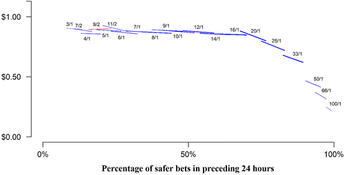
Notes. Each line segment plots the OLS relation between returns to a $1 bet and percentage of safer bets in the preceding 24 hours for 1 of the 20 most common values of odds. Downward-sloping line segments are colored blue. Upward-sloping line segments are colored red. Each line segment extends through the interquartile range of the percentage of safer bets for that value of the odds. Thickness is proportional to the number of observations (ranging from 25,000 to 85,000 and totaling more than a million).
To estimate the average effect of contextual odds, we regress parimutuel returns to a $1 bet against the percentage of safer bets in the preceding 24 hours along with separate intercepts for each of the 98 observed values of betting odds and cluster standard errors at the race level. Effectively, this estimates the average slope of the regression lines in Figure 2 (but for all 98 values of the odds). It indicates a 31-cent decrease in the expected value of a $1 bet if we could hold its odds fixed when shifting it from safest to riskiest in the preceding 24 hours (t = −7.6). This relation is robust to controls for observables, including a variety of horse and race characteristics (see the online supplement for details).
According to our payoff contrast hypothesis, only odds on other races likely to be salient to gamblers should affect demand. We sharpen our causal inference with a placebo: the distribution of odds in the 24 hours following each race, which should capture the same unobserved market conditions as odds in the preceding 24 hours but could not affect bettors. When we estimate the same regression that we report earlier, replacing the percentage of safer bets in the preceding 24 hours with the percentage of safer bets in the following 24 hours,8 we no longer estimate a significant relation with parimutuel returns (B = −6 cents, t = −1.5), which rules out many alternative accounts of the relation with preceding odds.
Figure 3 reports the results of simultaneously regressing realized returns against the percentage of safer bets in each 24-hour period from 90 days before to 90 days after the target race along with separate intercepts for each of the 98 observed values of betting odds and clustering standard errors at the race level.9 It shows that the percentage of safer bets in the immediately preceding 24 hours is a stronger predictor of demand (B = −31, SE = 6) than the percentage of safer bets in any other 24-hour period with the percentage of safer bets in the period from 48 to 72 hours before the race the second strongest (B = −18, SE = 5).
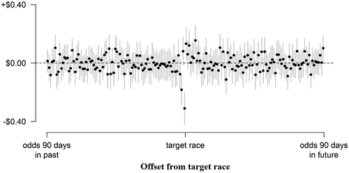
Notes. Coefficients from the simultaneous regression of returns to a $1 bet against the percentage of safer bets within 180 24-hour periods (after including intercepts for each individual value of the betting odds). Error bars represent 95% confidence intervals, clustered by race.
In addition to directly estimating the effect of safer contextual gambles, we also find evidence of contextual rank dependence from aggregate tests involving the median and variance of odds from the preceding 24 hours. The online supplement provides details.
To estimate the model of payoff contrast described in Section 3, we assume a representative agent with unbiased beliefs who bets one unit on the horse with the highest subjective expected value. We assume functional forms for the probability weighting function and value function :
This results in a total of five estimable parameters : the scaling factor from Equation (1), the distance sensitivity parameter from Equation (2), the sensitivity and pessimism parameters and from Equation (3) (Prelec 1998), and the exponent to allow for changing marginal utility in Equation (4).
Imposing constraints on the estimable parameters allows comparison between four theoretically interesting models. Expected utility is the special case in which the scaling factor and the probability weighting parameters and are each constrained to equal one so that and there are no effects of context. Relaxing constraints on the probability weighting parameters and maintaining the constraint on the scaling factor gives a model of decision weighted utility—the leading representative agent model of the longshot bias. A “pure” payoff contrast model results from constraining the value function parameter and the probability weighting parameters and to each equal one so that and , while allowing the scaling factor and the distance sensitivity parameter to vary. This models a representative agent who only deviates from maximization of expected value because of contrast with context. When all five parameters vary freely, we model a representative agent who is simultaneously affected by changing marginal utility, nonlinear decision weighting, and payoff contrast.
Finally, we assign a value of zero to the loss of a bet and we assume that the market reaches equilibrium—that the closing odds make all horses within a race equally attractive to the representative agent. We assign a value of to the ex ante subjective expected value of a unit bet on the horse in finishing position i to win race j and pay out in the context of potential payoffs from other races in the preceding 24 hours.
We solve for the representative agent’s decision weights ,
We then solve for the model-estimated true winning probabilities by inverting the probability-weighting function and setting values of that constrain winning probabilities to sum to one within each race.
Finally, we set free parameters to maximize the joint probability of winning horses across the n = 126,117 races that have other races in the preceding 24 hours and don’t end in a tie.
Table 1 reports parameter estimates and log-likelihoods under the four combinations of constraints described above. The expected and decision-weighted utility specifications (specifications I and II) replicate previous findings that probability weighting adds significant incremental validity over and above changing marginal utility (). Parameter values are roughly consistent with reports from previous authors estimating similar models in other horse racing data (Jullien and Salanié 2000, Snowberg and Wolfers 2010).
|

Table 1. Parameter Estimates and Log-Likelihoods from Four Models of the Probability That a Horse Will Win Its Race
| I | II | III | IV | |
|---|---|---|---|---|
| Changing marginal utility () | 1.178 0.004 | 0.778 0.014 | 1 | 0.949 0.021 |
| Probability sensitivity () | 1 | 0.769 0.013 | 1 | 1.048 0.052 |
| Pessimism () | 1 | 1.011 0.010 | 1 | 0.916 0.023 |
| Scaling factor () | 1 | 1 | 1.041 0.005 | 1.058 0.023 |
| Distance sensitivity () | – | – | 0.745 0.042 | 0.704 0.052 |
| −2 × log-likelihood | 474,755 | 474,467 | 474,409 | 474,408 |
Notes. Subscripts are standard errors. Values without standard errors are constrained. The distance sensitivity parameter has no value when the scaling factor is constrained to one (because its value has no effect when the scaling factor is one).
Specification III estimates our pure payoff contrast model. Because the decision-weighted utility and pure payoff contrast specifications are nonnested, we use Vuong’s (1989) closeness test to compare their accuracy. Despite using fewer free parameters than decision-weighted utility, the pure payoff contrast fits the data significantly better (z = 5.2). Finally, specification IV allows probability weighting and changing marginal utility in addition to payoff contrast. It finds no significant improvement over and above pure payoff contrast ().
In both specifications that allow for payoff contrast (specifications III and IV), the scaling factor is significantly greater than one, confirming contrast. The distance sensitivity parameter is significantly less than one, indicating diminishing sensitivity to distance from contextual payoffs, but significantly greater than zero. The supplement presents simulation results showing that estimates of the distance sensitivity parameter are slightly upward-biased by error in the reference set assumption (and our reference set assumption cannot possibly be error-free). However, this bias is too small for our estimate of the distance sensitivity parameter to be consistent with decision by sampling’s binary comparison assumption.
Figure 4 plots observed betting returns against model-predicted betting returns. It clearly replicates previous reports that conventional representative agent models cannot simultaneously capture both the steepness of the longshot bias and the fact that there are so few profitable betting opportunities among favorites (Gandhi and Serrano-Padial 2015, Green et al. 2020).
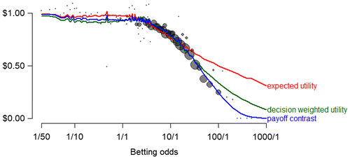
Notes. Black dots are observed average returns to $1 bets on each of the 98 values of the betting odds with area directly proportional to the number of observations at each value (ranging from 2 to about 85,000 and totaling almost 1.3 million). Solid lines are model predictions of the same data based on maximum likelihood estimates of specifications I, II, and III from Table 1.
Most importantly, Figure 4 shows that the two-parameter, pure payoff contrast model captures the full pattern. Among the 20 most common values of the odds, the largest discrepancy between the observed and model-predicted win rate is half of a percentage point—almost as accurate as we would expect from the true model. That is, only 10 of the 98 total odds values reject their model-predicted win rates at the 0.05 level; only two reject at the 0.01 level (4/1 and 22/1), and no value of the odds rejects the model prediction at the 0.005 level. This rejection rate is only slightly higher than we would expect from the true model of the relation between win rate and odds.
Unfortunately, because contextual gambles are always present in gambling markets, it is difficult to use field data to test our payoff contrast hypothesis’s second prediction: that preferences shift toward longshots when contextual gambles become available for comparison. Nonetheless, we can ask whether the longshot bias is weaker when comparisons to other bets are less salient, for example, in the morning when bettors are less likely to have recently considered odds on preceding races. Previous researchers report that the longshot bias is particularly strong on the last race of the day (McGlothlin 1956, Ali 1977). We find that the relation between time of day and magnitude of the longshot bias is roughly linear. The longshot bias is not just stronger than normal at the end of the day. It is also weaker than normal at the beginning of the day (see the online supplement for details). The next section reports a simple experimental test of the predicted change in longshot preferences.
5. A Preference Reversal When Contextual Gambles Are Available for Comparison
We manipulate the presence of contextual gambles to demonstrate a preference reversal as demand shifts toward longshots when contextual gambles become available for comparison. We randomly assigned 2,008 participants (MTurk workers) to consider two gambles in one of two gamble order conditions. One gamble offered one-to-one odds on rain in Seattle, and the other offered 39-to-1 odds on rain in Las Vegas. In one condition, the Seattle gamble preceded the Las Vegas gamble. In the other condition, the Las Vegas gamble preceded the Seattle gamble. The two gambles were always presented on separate screens, and participants could never go back to the first gamble after advancing to the second (Table 2).
|
Table 2. Seattle/Las Vegas Experimental Materials
| Seattle first condition (n = 993) | Las Vegas first condition (n = 1,015) | |
|---|---|---|
| Trial 1 | Would you bet $10 to win $20 if it rains on November 15 in Seattle, Washington? | Would you bet $10 to win $400 if it rains on November 15 in Las Vegas, Nevada? |
| Trial 2 | Would you bet $10 to win $400 if it rains on November 15 in Las Vegas, Nevada? | Would you bet $10 to win $20 if it rains on November 15 in Seattle, Washington? |
Our payoff contrast hypothesis predicts that, on the second trial of the experiment, the contrast with the first trial potential payoff increases the attractiveness of the longshot Las Vegas gamble relative to the safer Seattle gamble. We find exactly that. On the first trial, the Seattle gamble is accepted more than the Las Vegas gamble (77% versus 68%, z = 4.1), but on the second trial, it is accepted less often (57% versus 63%, z = 2.4).10
So far, we have presented evidence that our scaling model captures the shape of the longshot bias and evidence of contextual rank dependence and change in longshot preferences. Further, the predicted moderation by presentation format is evidenced in betting exchanges,11 which reveal a longshot bias when odds are presented in the standard format (Kopriva 2015, Abinzano et al. 2016) but not when presented as the price to buy a $1 payoff if an event obtains: a context in which the prices not only resemble probabilities, ranging between zero and one (dollars), but in which they can be roughly interpreted as probabilities (Wolfers and Zitzewitz 2006). Indeed, in these state price security contexts, favorites are slightly overpriced (Tetlock 2004, Cowgill et al. 2009, Berg and Rietz 2019).
In the next section, we manipulate context and presentation format to test all three predictions of our payoff contrast hypothesis within the same experiment. We then use individual participant-level variation in contrast effects to demonstrate the link between the contextual rank dependence we find in the field and the change in longshot preferences we demonstrate in the laboratory. Finally, we reestimate our scaling model and show that it accurately captures the change in longshot preferences across experimental trials.
6. An Experiment Testing All Three Predictions of the Payoff Contrast Hypothesis
Using the 51 largest U.S. cities as our natural reference class, we created 51 hypothetical rain bets. We use rain bets because they allow us to manipulate whether probability information is explicit (probability of rain is provided in the question statement) or implicit and inferred by participants from their knowledge of geography and weather. Each bet was priced at $10, and each had an expected value of $30 based on historical probability of rain in that city (see the online supplement for detailed materials); 3,019 participants (MTurk workers) were each presented with 21 rain bets sequentially on separate screens. The first 20 rain bets were independent random draws from the set of rain bets, excluding New York City. The 21st rain bet was always New York City.12 Participants were told that they should consider each bet separately and were informed before beginning that cities with higher potential payoffs have lower probabilities of rain.
Rain bets were randomly assigned on each trial (with replacement), allowing us to use random variation in the rain bets assigned to previous trials to test our contextual rank-dependence prediction. The same random assignment also ensures that the distribution of gambles on the first trial is the same as the distribution of gambles on later trials, allowing us to test the predicted shift toward longshots when preceding contextual gambles are available for comparison. Finally, we manipulated between subjects whether the probability of rain was left implicit or made explicit to create one condition in which the betting odds format mirrors the betting market (potential payoffs are easier to compare than winning probabilities) and one condition in which exact probabilities are available for easy comparison. This allows us to test the predicted moderation-by-presentation format: that providing explicit winning probabilities creates countervailing contrast effects, moderating the effect of context and reducing or even reversing a longshot bias.
Implicit Probability Condition (N = 1,505): Would you bet $10 to win $X if it rains on July 15 in C?
Explicit Probability Condition (N = 1,514): There is aP% chance that it will rain on July 15 in C. Would you bet $10 to win $X if it does?
The top panel of Figure 5 presents a test of contextual rank dependence. It plots the gamble acceptance rate against the percentage of safer gambles encountered on prior trials separately for each rain bet within the implicit probability condition of our experiment. Just as in the horse racing market, demand for a given bet is higher if contextual gambles are safer, providing further support for the contextual rank-dependence prediction. The correlation is positive for 41 out of 51 individual rain bets, and on average, a given bet’s acceptance rate increases by 1.2 percentage points for every 10-point increase in the percentage of safer gambles encountered on prior trials (t = 3.8, including separate intercepts for each of the 51 rain bets and clustering standard errors by participant here and in all following analyses).
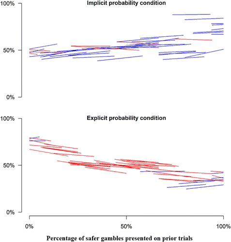
Notes. Each line segment plots the OLS relation between acceptance rate and percentage of safer gambles presented on prior trials for 1 of the 51 rain bets. Upward-sloping line segments are colored blue. Downward-sloping line segments are colored red. Each line segment extends through the interquartile range of the percentage of safer bets for that rain bet.
The top panel of Figure 6 presents a test of the predicted change in longshot preferences. It separates the first trial (in which there are no preceding gambles to provide context) from the next 19 (in which memory of prior gambles is available for comparison) and plots the relation between rainfall probability and acceptance rate within the implicit probability condition. There is no longshot bias on the first trial, but a longshot bias becomes apparent on later trials, replicating the result of the Seattle/Las Vegas experiment presented in the previous section and providing further support for the predicted change in longshot preferences (β = −9, SE = 8 versus β = −43, SE = 3; t = 4.4).
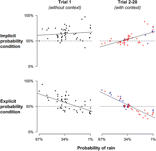
Notes. Each point plots the percentage of participants betting on rain in a city against the probability of rain in that city. The right panel uses downward-facing red triangles to indicate rain bets whose acceptance rates decreased after trial 1 and upward-facing blue triangles to indicate rain bets whose acceptance rates increased after trial 1.
Finally, the bottom panels of Figures 5 and 6 provide tests of the predicted moderation by presentation format. They show that the explicit probability condition not only moderates the effect of contextual gambles, but reverses it. The bottom panel of Figure 5 shows that contextual rank dependence reverses; demand for a given bet now falls as the percentage of safer gambles encountered on prior trials increases (β = −1.9%, t = −6.1). The bottom panel of Figure 6 shows that the change in longshot preferences also reverses. The presence of contextual gambles now shifts demand toward favorites (β = 50, SE = 7 versus β = 73, SE = 3; t = 3.1), again reversing the effect of context that we observe in the implicit probability condition and confirming the predicted moderation by presentation format.
Next, we divide each condition between subjects who predominantly contrast gambles along the payoff dimension and subjects who predominantly contrast gambles along the probability dimension to provide further evidence that the change in longshot preferences depends on contrasts against preceding gambles. We limit this individual level analysis to the 2,510 subjects who respond to all 21 gambles and vary in their responses (sometimes accepting and sometimes rejecting).
The fact that we only observe 21 choices per subject means that we do not have enough observations to include separate intercepts for each possible current gamble, which requires a different procedure to distinguish the effects of contextual gambles from the effects of the current gamble. For each rainfall gamble, we calculate the percentile rank among the full distribution of potential payoffs. The mean payoff percentile rank of gambles presented on prior trials equals the probability that a random draw from prior trials exceeds the potential payoff of a random draw from the full distribution. This allows us to replace the percentage of safer gambles on prior trials with an unbiased estimate of it that is unrelated to the gamble that happens to be assigned to the current trial.
A negative correlation with gamble acceptance indicates that the subject is more likely to accept the current bet when previously observed gambles were likely to have a lower payoff, suggesting that the subject predominantly contrasts gambles along the payoff dimension. A positive correlation indicates that the subject is more likely to take the current bet when previously observed gambles were likely to have a lower probability, suggesting that the subject predominantly contrasts gambles along the probability dimension.
Figure 7 separates subjects within each presentation format condition into the two contrast segments described. It presents the relation between rainfall probability and gamble uptake on trial 1 and trials 2–20 separately for each contrast segment of each condition. On trial 1, the relation between rainfall probability and gamble uptake already varies between conditions but not between contrast segments within a condition. Critically, the two contrast segments diverge on later trials as subjects who contrast payoffs shift toward riskier bets, whereas subjects who contrast probabilities shift toward safer bets. The relation between rainfall probability and gamble uptake changes in the predicted direction from trial 1 to trials 2–20 in both contrast segments of both conditions, and those changes attain statistical significance in three out of four (ts = −5.5, 1.2, −2.9, and 5.3),13 providing strong support for our payoff contrast hypothesis.
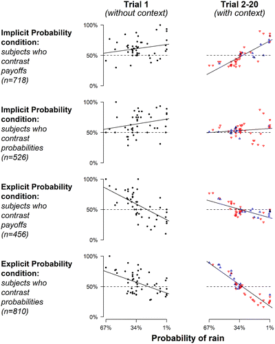
Notes. Each point plots the percentage of participants betting on rain in a city against the probability of rain in that city. The right panel uses downward-facing red triangles to indicate rainfall bets whose acceptance rates decreased after trial 1 and upward-facing blue triangles to indicate rainfall bets whose acceptance rates increased after trial 1.
We model the subject’s betting decision as evaluating whether exceeds the absolute value of . In the implicit probability condition, we model contrast between payoffs: . In the explicit probability condition, we model contrast between probabilities: . Unlike the market data, these data reveal not just the relative popularity of longshots to favorites, but also their actual levels of popularity. So we allow for loss aversion (Kahneman and Tversky 1979) to explain the overall bet rate and a Luce (1959) model to transform utility differences into choice probabilities. Unfortunately, there is only one level of loss (−10), and winning probabilities are perfectly correlated with potential payoffs, so we set the pessimism parameter from Prelec’s (1998) probability-weighting function to equal one and take the parameter estimates with a grain of salt.
Table 3 reports maximum likelihood estimates of a null specification without contextual contrast and of a full specification that allows contextual contrast. Because the choices are clustered by respondent, we use a cluster bootstrap to estimate the standard deviations of parameter estimates as well as the standard deviations of log-likelihood ratios for comparisons between specifications. As strongly implied by the reduced form tests reported, the full specification fits the data significantly better than the null specification in both the implicit (z = 3.0) and explicit (z = 3.1) probability condition. Further, the distance-sensitivity parameter is significantly less than one, indicating diminishing sensitivity to distance from reference values but significantly greater than zero, once again rejecting decision by sampling’s assumption of binary comparison. The supplement reports similar results after reestimating the model, assuming probability-weighting parameter values reported by Baillon et al. (2020) or Abdellaoui et al. (2011).
|
Table 3. Parameter Estimates and Log Likelihoods from a Model of Gamble Acceptance Probability That Includes Contextual Contrast and a Model That Doesn’t
| Implicit probability condition | Explicit probability condition | |||
|---|---|---|---|---|
| Null | Full | Null | Full | |
| Logit sensitivity () | 0.317 0.083 | 0.435 0.055 | 1.229 0.210 | 0.807 0.085 |
| Changing marginal utility () | 1.048 0.013 | 0.993 0.013 | 0.802 0.021 | 0.861 0.019 |
| Loss aversion () | 3.298 0.091 | 2.918 0.084 | 1.958 0.059 | 2.225 0.086 |
| Probability sensitivity () | 1.013 0.005 | 0.993 0.007 | 0.896 0.016 | 0.925 0.011 |
| Payoff contrast | ||||
| Scaling factor () | 1 | 1.016 0.007 | 1 | 1 |
| Distance sensitivity () | – | 0.158 0.066 | – | – |
| Probability contrast | ||||
| Scaling factor () | 1 | 1 | 1 | 1.063 0.020 |
| Distance sensitivity () | – | – | – | 0.246 0.067 |
| −2 × log-likelihood | 42,570 | 42,440 | 41,953 | 41,800 |
Note. Subscripts are bootstrap standard errors, clustered by participant.
Finally, Figure 8 plots the correlation between rainfall probability and gamble acceptance separately for each trial of each condition. Black dots are observed correlations. Blue lines are predicted correlations based on simulated choices from the full specification. In both cases, correlations start close to zero and fan out, quickly at first and then more slowly. The correlation between predicted and observed is 0.53 in the explicit probability condition and 0.87 in the implicit probability condition. This correspondence is impressive because the model never sees the experimental trial; all predictions simply reflect the parameter values reported in the full specification from Table 3.
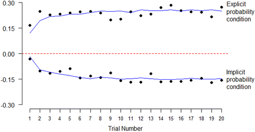
Notes. Black dots are the observed correlations between rainfall probability and gamble uptake on each trial of each condition. Blue lines are average correlations from 1,000 simulations of the full specification from Table 3 (with appropriate transformation to Fisher’s z and back again).
7. General Discussion
The longshot bias provides a striking counterexample to the typical assumption that riskier assets have higher expected returns (Sharpe 1964, Lintner 1965). Its existence in almost every odds-based gambling market is often interpreted as evidence of nonlinear probability weighting (Camerer 1988). We advance a novel hypothesis: the longshot bias results from the bettor’s tendency to contrast potential payoffs whenever that is easier than comparing the probabilities of winning. We exploit natural variation in a 24-year series of historical betting data and random assignment in two large-sample betting experiments to test three predictions from our payoff contrast hypothesis: (1) that demand for a given bet increases with the percentage of safer bets observed recently, (2) that the longshot bias emerges when there are contextual odds for comparison, and (3) that the effect attenuates or even reverses when the decision environment facilitates countervailing contrasts between probabilities.
We find evidence that preferences are determined not only by a bet’s own odds, but by the position of those odds within the distribution of recently observed odds. Further, this cross-race comparison between gambling odds is asymmetric in an important way. Although we expect bettors to value both high potential payoffs and high probabilities of winning, they only seem to compare across races along the payoff dimension. This holds until we make the winning probabilities explicit in our final study, at which point people switch and begin to contrast bets along the probability dimension. We could describe this general pattern in terms of Kahneman and Frederick’s (2002) model of attribute substitution, as substituting an easier heuristic judgment of relative payoff or relative probability for a more difficult cross-modal judgment that requires the decision maker to integrate payoffs with probabilities.
Rather than aggregating reference sets into reference points and modeling a single comparison, we follow the theory of decision by sampling to average over individual comparisons with each member of the reference set. This feature of decision by sampling appears to be correct, because when we reverse the order of operations (now averaging before comparing), model fit degrades significantly in both the laboratory (implicit probability condition: z = 1.5; explicit probability condition: z = 3.2) and the field (z = 2.1). On the other hand, our scaling model rejects decision by sampling’s binary comparison assumption, but provides support for a weaker version of it: diminishing sensitivity to distance from individual members of the reference set. See Niedrich et al. (2001) or Janiszewski and Lichtenstein (1999) for further discussion. For a different modeling perspective, see Bordalo et al. (2012, 2020).
In some cases, there is a potential alternative explanation of our findings in terms of assimilation toward previously considered winning probabilities. Bettors who shrink estimated winning probabilities toward the distribution of winning probabilities from recent races might create something resembling the patterns we observe. However, a belief-assimilation alternative would not be able to explain the contrasts between probabilities in the explicit probability condition of our many-city rain-betting experiment. Further work should manipulate gamble payoffs and probabilities independently to better differentiate our payoff contrast model from a belief-assimilation alternative.
We also consider an intertemporal substitution-based interpretation of our findings. If gamblers have quotas on the number of gambles to accept, a more attractive preceding gamble could make gamblers less likely to accept the current gamble, not because of any comparison with the preceding gamble, but because they already took the preceding gamble, and don’t want to take too many. For this alternative to explain our results, the attractiveness of gambles must covary with their riskiness. Although attractiveness and riskiness do covary in our many-city rain-betting experiment, they don’t covary on the first trial of its implicit probability condition, leaving intertemporal substitution unable to account for an effect of trial 1 on trial 2 in that condition (and there is a large effect). Additionally, the effect of prior trial riskiness is robust to controlling for measures of prior trial attractiveness (see supplement for details). Finally, intertemporal substitution makes the wrong prediction for the Seattle/Las Vegas experiment, in which the Las Vegas gamble is elevated relative to the Seattle gamble on the second trial despite the Las Vegas gamble following a more popular gamble than Seattle does. Intertemporal substitution can capture the strengthening of a relation that already exists on earlier trials but cannot capture the observed preference reversal.
In parimutuel markets, odds equate average attractiveness across available gambles, so straightforward versions of an intertemporal substitution alternative cannot explain our field data. However, if some bettors only bet on favorites and other bettors only bet on longshots, demand for longshots could accumulate when longshots are rare on preceding days. There are many reasons to be skeptical of alternative explanations along these lines. First, our main analysis is of the percentage of safer bets rather than the number of favorites, so such an alternative needs demand to vary by percentage of favorites. Second, we find no effects of recent longshot victories, which would elevate demand for longshots on subsequent days if longshot bettors were budget-constrained. Most importantly, we find the sign is wrong for such an interpretation. Instead of a decrease in the demand for favorites after a period with an abnormally high percentage of favorite odds, we find an increase in the demand for favorites after a period with an abnormally high percentage of favorite odds (see the online supplement for details).
Finally, our reliance on bookmaker odds to proxy for parimutuel odds in the horse racing market opens the possibility that the context effects we observe reflect an effect on the bookmaker rather than on the gambling public. Although we assume most market biases reflect the least sophisticated participants, the bookmaker-based interpretation is tempting here because the bookmaker is guaranteed exposure to the full set of contextual gambles. However, if this were the case, we would expect a larger effect on returns to betting with the bookmaker than in the parimutuel market. Instead, for most specifications, we find similar magnitude effects on returns to betting in either market, and in some specifications, we find the opposite: a stronger effect of contextual rank dependence on returns in the parimutuel market than on returns in the bookmaker market. The online supplementary materials provide details. Most importantly, the bookmaker alternative cannot explain our experimental data.
Researchers offer many plausible explanations for the longshot bias, and we generally assume any pattern this robust has multiple causes. Although our scaling model fully captures the shape of the longshot bias in the field data and does an adequate job of describing the change in risk preference over the course of our multicity rainfall betting experiment, we make no claim that the pure two-parameter version of our model is a complete description of decision making under risk. Even allowing for payoff contrast, we estimate substantial loss-aversion parameters in both conditions of our multicity rainfall betting experiment. We also see clear evidence of standard probability weighting and diminishing sensitivity to potential payoffs in the explicit probability condition of our multicity rainfall betting experiment. It seems likely that the longshot bias is not only determined by the psychological processes on which we focus, but also by other factors, such as the aggregation of bettors with heterogenous beliefs (Gandhi and Serrano-Padial 2015, Green et al. 2020) and traditional context-invariant probability weighting.
In addition to providing a novel explanation for the longshot bias, the context effects we document here raise more general concerns for utility calibrations with repeated trials in laboratory data. Empiricists who attempt to estimate stable preference functions usually present many gambles to each subject, assuming that the random ordering of options ensures that previously observed gambles have no systematic effect on current choices (e.g., Preston and Baratta 1948, Tversky and Kahneman 1992, Gonzalez and Wu 1999). The context effects that we document here suggest that calibrations based on repeated choices across many gambles may not generalize to gambles presented in isolation.
The authors thank Shane Frederick, Steve Malliaris, Reid Hastie, Devin Pope, Paul Braverman, Nicholas Barberis, Edward Kaplan, George Wu, and Amanda Levis for discussion and feedback. The authors thank flatstats.co.uk for providing historical betting data.
1 It’s not completely novel. In his initial documentation of the longshot bias, Griffith (1949) considered and dismissed a version of our explanation because the longshot bias’s inflection point does not correspond with the geometric mean of the odds distribution as might be predicted by Helson’s (1948) adaptation-level theory.
2 This is at least purportedly irrelevant. See Kamenica (2008), Sher and McKenzie (2014), or Wernerfelt (1995) for further discussion.
3 There are also numerous examples of context effects on scale ratings and category judgments (Parducci 1965, 1968), but it is not clear whether they reflect changing preferences or changing scale usage and category definition (Sherman et al. 1978). Contrast between perceptual phenomena such as the size of a circle (Massaro and Anderson 1971) or the intensity of a light source (Diamond 1953) is also well-established but less relevant to our findings. Reference price effects in consumer goods markets may be more consistent with rational inference about the future price of a good (Muth 1961, Winer 1986, Bell and Lattin 2000).
4 Both the Walasek and Stewart (2015) and Stewart et al. (2015) results can be interpreted in multiple ways (Alempaki et al. 2019; André and de Langhe 2021a, b; Walasek et al. 2021).
5 Effects of wage rank on life satisfaction (Boyce et al. 2010), sequential decision making in speed-dating contexts (Bhargava and Fisman 2014), and anchoring in a variety of contexts including real estate markets (Simonsohn and Loewenstein 2006), commuting distances (Simonsohn 2006), and art auctions (Beggs and Graddy 2009) may reflect a similar underlying contrast mechanism (Frederick and Mochon 2012).
6 Unlike prospect theory (Kahneman and Tversky 1979), whose reference point is determined by the status quo, or prospect theory variants that allow multiple reference points based on probabilistic endowments (Kőszegi and Rabin 2006, 2007; Schmidt et al. 2008), the decision by sampling framework (Stewart et al. 2006) allows for effects of attribute values that have merely been observed by the decision maker.
7 The number of horse starts for analysis (1,298,373) is after excluding 22 horse starts with overround greater than or equal to two and 556 horse starts with overround less than or equal to one because overround outside of this range probably indicates a data error.
8 We also switch from excluding 10,059 horse starts without any races in the preceding 24 hours to excluding 10,095 horse starts without any races in the following 24 hours.
9 This analysis excludes the first and last 90 days of data (11,484 horse starts), but includes all other observations, avoiding division by zero when calculating the percentage of safer bets by adding 0.5 to the numerator and one to the denominator.
10 We suspect that the main effect of trial reflects a reachability bias on first trial binary choices as extensively documented by Bar-Hillel et al. (2014). It may also reflect loss aversion in riskless choice and contrast effects on both the payoff and probability dimensions (Tversky and Kahneman 1991).
11 Rather than a central pool or a bookmaker taking the opposite side of each bet, betting exchanges use an order book to match gamblers on either side of each bet, just as in a stock exchange.
12 We held the 21st bet fixed because allowing it to vary does nothing to identify effects on later gambles, and keeping it fixed allows a high-power test of recency and primacy effects. Surprisingly, there is no evidence of recency effects over the 21-gamble series, but strong evidence of primacy effects (see the online supplement for details).
13 The subjects who appear to contrast probabilities in the implicit probability condition are the only group that doesn’t change significantly. They are also the only group that implies a contrast between quantities that are not explicitly provided.
References
- (2011) The rich domain of uncertainty: Source functions and their experimental implementation. Amer. Econom. Rev. 101(2):695–723.Crossref, Google Scholar
- (2016) Game, set and match: The favourite-long shot bias in tennis betting exchanges. Appl. Econom. Lett. 23(8):605–608.Crossref, Google Scholar
- (2019) Reexamining how utility and weighting functions get their shapes: A quasi-adversarial collaboration providing a new interpretation. Management Sci. 65(10):4841–4862.Link, Google Scholar
- (1977) Probability and utility estimates for racetrack bettors. J. Political Econom. 85(4):803–815.Crossref, Google Scholar
- André Q, de Langhe B (2021a) No evidence of loss aversion disappearance and reversal in Walasek and Stewart (2015). J. Experiment. Psych.: General 150(12):2659–2665.Google Scholar
- André Q, de Langhe B (2021b) How (not) to test theory with data: Illustrations from Walasek, Mullett, and Stewart (2020). J. Experiment. Psych.: General 150(12):2671–2674.Google Scholar
- (2020) Searching for the reference point. Management Sci. 66(1):93–112.Link, Google Scholar
- (2014) “Heads or tails?”—A reachability bias in binary choice. J. Experiment. Psych. Learn. Memory Cognition 40(6):1656–1663.Crossref, Google Scholar
- (2009) Anchoring effects: Evidence from art auctions. Amer. Econom. Rev. 99(3):1027–1039.Crossref, Google Scholar
- (2000) Looking for loss aversion in scanner panel data: The confounding effect of price response heterogeneity. Marketing Sci. 19(2):185–200.Link, Google Scholar
- (2019) Longshots, overconfidence and efficiency on the Iowa electronic market. Internat. J. Forecasting 35(1):271–287.Crossref, Google Scholar
- (2014) Contrast effects in sequential decisions: Evidence from speed dating. Rev. Econom. Statist. 96(3):444–457.Crossref, Google Scholar
- (1992) Violations of monotonicity and contextual effects in choice-based certainty equivalents. Psych. Sci. 3(5):310–315.Crossref, Google Scholar
- (2012) Salience theory of choice under risk. Quart. J. Econom. 127(3):1243–1285.Crossref, Google Scholar
- (2020) Memory, attention, and choice. Quart. J. Econom. 135(3):1399–1442.Crossref, Google Scholar
- (2010) Money and happiness: Rank of income, not income, affects life satisfaction. Psych. Sci. 21(4):471–475.Crossref, Google Scholar
- (1988) Prospect theory in the wild: Evidence from the field. Advances in Behavioral Economics, 148.Google Scholar
- (2019) From aggregate betting data to individual risk preferences. Econometrica 87(1):1–36.Crossref, Google Scholar
- Cowgill B, Wolfers J, Zitzewitz E (2009) Using prediction markets to track information flows: Evidence from Google. Das S, Ostrovsky M, Pennock D, Szymanksi B, eds. Auctions, Market Mechanisms and Their Applications. AMMA 2009. Lecture Notes of the Institute for Computer Sciences, Social Informatics and Telecommunications Engineering, vol. 14 (Springer, Berlin, Heidelberg).Google Scholar
- (1953) Foveal simultaneous brightness contrast as a function of inducing, and test-field luminances. J. Experiment. Psych. 45(5):304–314.Crossref, Google Scholar
- (2014) The limits of attraction. J. Marketing Res. 51(4):487–507.Crossref, Google Scholar
- (2012) A scale distortion theory of anchoring. J. Experiment. Psych. General 141(1):124–133.Crossref, Google Scholar
- (2015) Does belief heterogeneity explain asset prices: The case of the longshot bias. Rev. Econom. Stud. 82(1):156–186.Crossref, Google Scholar
- Green E, Lee H, Rothschild DM (2020) The favorite-longshot Midas. Jacobs Levy Equity Management Center for Quantitative Financial Research Paper, Social Science Research Network. Preprint submitted August 12, https://ssrn.com/abstract=3271248.Google Scholar
- (1949) Odds adjustments by American horse-race bettors. Amer. J. Psych. 62(2):290–294.Crossref, Google Scholar
- (1999) On the shape of the probability weighting function. Cognitive Psych. 38(1):129–166.Crossref, Google Scholar
- (2018) A tough act to follow: Contrast effects in financial markets. J. Finance 73(4):1567–1613.Crossref, Google Scholar
- (1948) Adaptation-level as a basis for a quantitative theory of frames of reference. Psych. Rev. 55(6):297–313.Crossref, Google Scholar
- (2009) The description–experience gap in risky choice. Trends Cognitive Sci. 13(12):517–523.Crossref, Google Scholar
- (2004) Decisions from experience and the effect of rare events in risky choice. Psych. Sci. 15(8):534–539.Crossref, Google Scholar
- (1996) The evaluability hypothesis: An explanation for preference reversals between joint and separate evaluations of alternatives. Organ. Behav. Human Decision Processes 67(3):247–257.Crossref, Google Scholar
- (1982) Adding asymmetrically dominated alternatives: Violations of regularity and the similarity hypothesis. J. Consumer Res. 9(1):90–98.Crossref, Google Scholar
- (1999) A range theory account of price perception. J. Consumer Res. 25(4):353–368.Crossref, Google Scholar
- (2000) Estimating preferences under risk: The case of racetrack bettors. J. Political Econom. 108(3):503–530.Crossref, Google Scholar
- Kahneman D, Frederick S (2002) Representativeness revisited: Attribute substitution in intuitive judgment. Gilovich T, Griffin D, Kahneman D, eds. Heuristics and Biases: The Psychology of Intuitive Judgment (Cambridge University Press, New York), 49–81.Google Scholar
- (1979) Prospect theory: An analysis of decision under risk. Econometrica 47(2):263–292.Crossref, Google Scholar
- (2008) Contextual inference in markets: On the informational content of product lines. Amer. Econom. Rev. 98(5):2127–2149.Crossref, Google Scholar
- Kopriva F (2015) Constant bet size? Don’t bet on it! Testing expected utility theory on betfair data. CERGE-EI Working Paper Series No. 545., Social Science Research Network.Google Scholar
- (2006) A model of reference-dependent preferences. Quart. J. Econom. 121(4):1133–1165.Crossref, Google Scholar
- (2007) Reference-dependent risk attitudes. Amer. Econom. Rev. 97(4):1047–1073.Crossref, Google Scholar
- (2004) Why are gambling markets organised so differently from financial markets? Econom. J. (London) 114(495):223–246.Google Scholar
- (1965) Security prices, risk, and maximal gains from diversification. J. Finance 20(4):587–615.Google Scholar
- (1959) Individual Choice Behavior (John Wiley, New York).Google Scholar
- (1995) Similarity and alignment in choice. Organ. Behav. Human Decision Processes 63(2):117–130.Crossref, Google Scholar
- (1971) Judgmental model of the Ebbinghaus illusion. J. Experiment. Psych. 89(1):147–151.Crossref, Google Scholar
- (1956) Stability of choices among uncertain alternatives. Amer. J. Psych. 69(4):604–615.Crossref, Google Scholar
- (1961) Rational expectations and the theory of price movements. Econometrica 29(3):315–335.Crossref, Google Scholar
- (2001) Reference price and price perceptions: A comparison of alternative models. J. Consumer Res. 28(3):339–354.Crossref, Google Scholar
- (1965) Category judgment: A range-frequency model. Psych. Rev. 72(6):407–418.Crossref, Google Scholar
- (1968) The relativism of absolute judgments. Sci. Amer. 219(6):84–93.Crossref, Google Scholar
- (1998) The probability weighting function. Econometrica 66(3):497–527.Crossref, Google Scholar
- (1948) An experimental study of the auction-value of an uncertain outcome. Amer. J. Psych. 61(2):183–193.Crossref, Google Scholar
- (1986) Betting and equilibrium. Quart. J. Econom. 101(1):201–207.Crossref, Google Scholar
- (2008) Third-generation prospect theory. J. Risk Uncertainty 36(3):203–223.Crossref, Google Scholar
- (2006) New Yorkers commute more everywhere: Contrast effects in the field. Rev. Econom. Statist. 88(1):1–9.Crossref, Google Scholar
- (2006) Mistake #37: The effect of previously encountered prices on current housing demand. Econom. J. (London) 116(508):175–199.Crossref, Google Scholar
- (1992) Choice in context: Tradeoff contrast and extremeness aversion. J. Marketing Res. 29(3):281–295.Crossref, Google Scholar
- (1964) Capital asset prices: A theory of market equilibrium under conditions of risk. J. Finance 19(3):425–442.Google Scholar
- (2014) Options as information: Rational reversals of evaluation and preference. J. Experiment. Psych. General 143(3):1127–1143.Crossref, Google Scholar
- (1978) Contrast effects and their relationship to subsequent behavior. J. Experiment. Soc. Psych. 14(4):340–350.Crossref, Google Scholar
- (2010) Explaining the favorite–long shot bias: Is it risk-love or misperceptions? J. Political Econom. 118(4):723–746.Crossref, Google Scholar
- (2009) Decision by sampling: The role of the decision environment in risky choice. Quart. J. Experiment. Psych. 62(6):1041–1062.Crossref, Google Scholar
- (2006) Decision by sampling. Cognitive Psych. 53(1):1–26.Crossref, Google Scholar
- (2015) On the origin of utility, weighting, and discounting functions: How they get their shapes and how to change their shapes. Management Sci. 61(3):687–705.Link, Google Scholar
- Tetlock P (2004) How efficient are information markets? Evidence from an online exchange. Working paper, Harvard University, Cambridge, MA.Google Scholar
- (1988) Anomalies: Parimutuel betting markets: Racetracks and lotteries. J. Econom. Perspect. 2(2):161–174.Crossref, Google Scholar
- (1991) Loss aversion in riskless choice: A reference-dependent model. Quart. J. Econom. 106(4):1039–1061.Crossref, Google Scholar
- (1992) Advances in prospect theory: Cumulative representation of uncertainty. J. Risk Uncertainty 5(4):297–323.Crossref, Google Scholar
- (2011) How incidental values from the environment affect decisions about money, risk, and delay. Psych. Sci. 22(2):253–260.Crossref, Google Scholar
- (1989) Likelihood ratio tests for model selection and non-nested hypotheses. Econometrica 57(2):307–333.Crossref, Google Scholar
- (2015) How to make loss aversion disappear and reverse: Tests of the decision by sampling origin of loss aversion. J. Experiment. Psych. General 144(1):7–11.Crossref, Google Scholar
- Walasek L, Mullett TL, Stewart N (2021) Acceptance of mixed gambles is sensitive to the range of gains and losses experienced, and estimates of lambda (λ) are not a reliable measure of loss aversion: Reply to André and de Langhe. J. Experiment. Psych.: General 150(12):2666–2670.Google Scholar
- Weitzman M (1965) Utility analysis and group behavior: An empirical study. J. Political Econom. 73(1):18–26.Google Scholar
- (1995) A rational reconstruction of the compromise effect: Using market data to infer utilities. J. Consumer Res. 21(4):627–633.Crossref, Google Scholar
- (1986) A reference price model of brand choice for frequently purchased products. J. Consumer Res. 13(2):250–256.Crossref, Google Scholar
- (2006) Interpreting Prediction Market Prices as Probabilities (No. w12200) (National Bureau of Economic Research).Crossref, Google Scholar

