A Behavioral Study of Assortment Planning
Abstract
Problem definition: We investigate the performance of human decision makers selecting which products to offer in a retail category, also known as assortment planning. In theory, this task requires the understanding of product interaction effects, such as cannibalization and inventory pooling benefits, and it involves solving a complex mathematical problem with stochastic and combinatorial components. Despite its practical importance, assortment planning is often performed by managers without any decision support system. In the academic literature, there have been no systematic studies of assortment planners’ behavior. Methodology/results: We develop a computer simulation of a market environment and conduct a behavioral experiment where subjects act as assortment planners. We analyze subjects’ decisions in different treatments by varying the decision support systems provided to them, the number of possible products to offer, the size of the expected-profit-maximizing assortment, and the default assortment. We observe systematic patterns in the subjects’ decisions; their variety choices appear to anchor at a value equal to half the size of the choice set (mean-anchoring bias) and to the size of the default assortment (status quo bias). Finally, we document some interesting effects of decision support information; its impact on performance appears to depend on how easily it can be interpreted. Managerial implications: Retailers should recognize that the size of the choice set influences the chosen assortment, leading to excessive variety when large and insufficient variety when small relative to optimal variety.
Funding: This work was supported by the Naveen Jindal School of Management at the University of Texas at Dallas.
Supplemental Material: The online appendix is available at https://doi.org/10.1287/msom.2020.0256.
1. Introduction
Assortment planning (i.e., selecting which products to offer in a given product category) is one of the key managerial responsibilities in the retail industry (Fisher and Vaidyanathan 2012). High variety can increase consumer spending (Deng et al. 2016) and build loyalty to the retailer (Corstjens and Lal 2000), but it comes at a cost; it increases inventory (because of the lack of pooling), leads to more overhead, and exacerbates product cannibalization. The multitude of factors that need to be considered and the combinatorial nature of the problem explain the extremely high computational complexity of the assortment optimization question (Kök et al. 2015).
Given this, it may seem paradoxical that this task is often performed by managers with little to no support from optimization algorithms. Although many companies use software to collect and visualize sales data, inference and recommendation tools are typically custom built and rely on human expertise (Davenport and Bean 2017, Davenport and Mahidhar 2018). For instance, Kesavan and Kushwaha (2020) describe a heuristic-based retailer’s decision support system that removes underperforming products, yet they report that managers override about half of these automated decisions. Although recent developments in artificial intelligence have increased interest in using algorithms for assortment planning, their adoption in retail remains rare (Rueter 2021).
Because assortment planning decisions rely heavily on managers’ judgments, we believe that it is important to understand how good human decision makers are at solving this problem, how exactly they arrive at their decisions, and ultimately, how to develop procedure recommendations that will help improve these decisions. However, to the best of our knowledge, there have been no systematic studies of assortment planners’ behavior in the academic literature.
In this study, we set out to obtain basic insights into this problem with a controlled laboratory experiment where human subjects assume the roles of assortment planners. We construct a deliberately simple market simulation, which allows us to control for factors that may introduce additional cognitive biases. We specifically focus on managers’ choice of products to offer in a given category (also known as assortment planning), and we abstract from other complications that can also affect decision biases, such as communication, forecasting, competition, pricing, and inventory stocking levels, which have been previously studied in the behavioral operations literature (see, e.g., Schweitzer and Cachon 2000, Moritz et al. 2014, Lee and Siemsen 2017, and Quiroga et al. 2019). Subjects participated in online experiments and were compensated based on their performance. Participants were recruited via the Amazon Mechanical Turk (mTurk) and Prolific platforms.
To develop the assortment planning conceptualization, we use the model introduced in the seminal paper by van Ryzin and Mahajan (1999), which has a simple and intuitive structure for the optimal assortment; it is a subset of the products that have the highest expected utility value for customers, which is a measure of each product’s popularity. Hence, this solution can be obtained by ranking the candidate products by popularity, similar to the aforementioned “culling” heuristic. We are interested in studying whether the human subjects arrive at this conclusion and if so, whether they include the optimal number of products in their assortment or suffer from systematic biases, like offering too much or too little variety. If such biases emerge, we are interested in understanding what causes them and how decision support systems can help guide subjects toward better decisions.
Our results suggest that subjects may perceive half of the size of the set of products that they are choosing from () as an anchoring point, effectively leading to larger chosen assortments as the total choice set size (n) increases. In Experiment 1, where subjects chose from a set of 7 products, their assortment sizes consistently fall between the optimal variety level and the midpoint of 3.5 products. They tended to select larger-than-optimal assortments when the optimal variety was two and smaller assortments when the optimal variety was six. In Experiment 2, where the optimal variety was five, subjects generally err on the smaller side across most treatments. However, all else equal, their assortment sizes are significantly larger when choosing from 20 products than when choosing from 7 products. These patterns point to the existence of a mean-anchoring bias, where subjects systematically gravitate toward an assortment size around half of the choice set size.
This finding is consistent with the cognitive preference for “average” solutions documented in related streams of the behavioral economics and operations literature, such as the compromise effect in decision theory (Simonson 1989) and the pull-to-center effect in the newsvendor problem (Schweitzer and Cachon 2000). Our results also suggest a status quo bias; subjects in our experiment appear to be anchoring to the starting assortment and choosing assortments that take less effort (in our experiment, fewer clicks) to reach.
We also investigate the effect of decision support tools on the performance of assortment planners. Our results suggest that decisions can be improved by analytical decision support tools but only if the information provided can be clearly interpreted by the subjects. Subjects who receive “intermediate” information that is supposed to make their task simpler but still requires analytical skills and effort to interpret in some instances did not perform better than those who did not receive any decision support information. Although we do not yet have a definitive explanation for this effect, our findings highlight a promising research direction for understanding how decision support tools influence managerial decision making.
Our study contributes to the literature in the following ways. (1) We develop an assortment planning problem conceptualization that is suitable for a controlled laboratory experiment; to the best of our knowledge, our paper is the first experimental study of an assortment planning problem. (2) We uncover systematic biases in the subjects’ solutions, which are reminiscent of biases observed in the behavioral operations literature (in particular, newsvendor experiments). (3) We explore the effects of different types of decision support systems on the subjects’ performance, and interestingly, we find that providing additional information does not always improve performance.
2. The Assortment Planning Problem
Our experiments utilize a computerized simulation of a market environment where subjects act as managers in charge of assortment selection at a retail store. The manager observes the set of possible products to offer on the market, which we refer to as the choice set, and from this set, the manager selects which products to offer, which we refer to as an assortment. Potential consumers observe the assortment and either buy one of the offered products or choose an outside option (i.e., do not buy). Consumer demand for each product is random and generated according to the multinomial logit (MNL) model (Ben-Akiva and Lerman 1985). Below, we introduce the problem formulation and discuss properties of the optimal solution for the classical assortment planning problem under the MNL demand model.
2.1. Market Demand Model
Consider a product category with potential products (i.e., choice set ). A retailer must choose a subset as her assortment to sell to a market of potential consumers (where is a fixed exogenous parameter). Each potential consumer observes S and either buys one unit of product or selects an outside option denoted by zero, which can be interpreted as buying from a firm’s competitor or not buying anything at all. The choices of potential consumers are probabilistic; they are independent and identically distributed according to the multinomial logit model.
In this model, consumer k has a utility for product j that can be expressed as , where is the “nominal” portion of the product utility, which we assume to be common to all consumers, and is a zero-mean random variable corresponding to the unobservable component specific to each consumer. Consumer k chooses a product j if , where refers to the outside option. The model assumes that the ’s are independent and identically distributed (i.i.d.) random variables following a Gumbel distribution: , where is Euler’s constant and is a scale parameter. With that assumption, the probability of choosing the product j, which we denote by , has a closed-form expression:
The retailer knows the popularity indices of all of the products in the choice set N that she is choosing from as well as the popularity index of the outside option. Without loss of generality, we order the products in the choice set N from the highest popularity index to the lowest: that is, .
Let be the random number of potential consumers who pick product j, which we refer to as the demand for product , and let be the random number of potential consumers who pick the outside option. Because the total number of potential consumers is , product demands follow a multinomial distribution with number of trials and success probability for product j. Therefore, the expected demand for product is , and the expected total demand for the assortment is equal to
From (2), observe that the retailer’s sales and consequently, profit are not additive; they increase in in a nonlinear fashion. This nonlinearity may present a significant challenge for the subjects, and on our side, it introduces particular complexities in empirically modeling their choices. We elaborate on this issue in Section 6.2 and Online Appendix EC.5. Further, adding a product to an assortment S increases the expected total demand for the assortment but decreases the expected individual demand for each existing product in the assortment, a phenomenon commonly referred to as product cannibalization.
Note that like most models of consumer choice used in assortment planning, the MNL model does not capture some specific effects, such as the confusion that excessive variety can cause in the mind of consumers (Iyengar et al. 2000) or other so-called context effects (Rooderkerk et al. 2011). For more discussion of the properties of the MNL model, see Ben-Akiva and Lerman (1985, chapter 5).
2.2. Retailer’s Profit Function
As in van Ryzin and Mahajan (1999), we assume that all products have identical profit margins denoted by r. The retailer incurs a fixed operational cost for every product included in the assortment regardless of the actual sales of that product, which is akin to a make-to-order setting or a scenario with free returns of unsold inventory to the manufacturer. We abstract from inventory considerations in order to focus our attention on the product selection decisions.
These assumptions on the retailer cost function are similar to those of the models in Gaur and Honhon (2006) and Ulu et al. (2012). In this case, the retailer’s expected profit (EP) from an assortment can be written as , where is given in ((2)) and |S| denotes the size of set S, which we refer to as the variety of assortment S.
In the general setting where products have different profit margins, finding the expected profit-maximizing (also known as optimal) assortment requires a full enumeration and comparison of profit values across all possible assortments (corresponding to all subsets of N). For the special case that we consider with identical profit margins, a well-known result from the assortment planning problem under the MNL model is that an optimal solution can always be found among assortments of the form for some , which are commonly referred to as popular sets (see van Ryzin and Mahajan 1999, Cachon et al. 2005, and Kök and Xu 2011). Further, it can be shown that the optimal assortment is such that adding the next popular product would cause expected profit to go down (i.e., the greedy method is optimal); as a result, a maximum of n assortments need to be compared in order to find the optimal one.
3. Research Questions
The primary goals of our study are to assess the performance of human decision makers at assortment planning and to explore possible systematic deviations in their solutions. Our primary focus is on the number of products that subjects include in their assortments and whether deviations from the optimal variety exhibit a systematic pattern: that is, whether the subjects would consistently offer too large or too small of assortments. One possibility is that decision makers tend to offer larger-than-optimal assortments, which would be consistent with the common view that there is excess variety in the retail industry (see, e.g., Boatwright and Nunes 2001). Another possibility is that decision makers may exhibit a mean-anchoring bias (i.e., they tend to lean toward “average” solutions); given a choice set with n possible products, where the optimal variety is , they would tend to choose assortment sizes between and some midpoint, which can be half of the size of the choice set . Human preferences are known to be reference dependent (Kahneman and Tversky 1979), and in many decision-making situations, the reference point is some “average” solution. For example, in behavioral operations and economics research, reference dependence manifests itself as the “compromise effect” (Simonson 1989) and “extremeness aversion” (Simonson and Tversky 1992) in consumer behavior and the “pull-to-center” effect in the newsvendor problem (Schweitzer and Cachon 2000).
To study this question, we conduct two experiments. In Experiment 1, we initially test our hypotheses, and in Experiment 2, we validate the robustness of our findings by replicating them in a somewhat different setup and further analyze some surprising phenomena observed in Experiment 1.
4. Experiment 1
4.1. Design and Procedure
In this experiment, every period has two stages corresponding to two different screens: the assortment selection stage and the results stage. In the assortment selection stage, the subjects select products by checking or unchecking a box next to a product label in a table format and hitting a “submit” button whenever they have completed the selection. When the chosen assortment is submitted, demand for each selected product is generated according to the MNL model described in Section 2.1, and the subjects move to the results stage, where the demand and profit values are displayed in a table format. After clicking on a button, the subjects move back to the assortment selection stage for the next period. This process is repeated for 25 independent periods, each having identical parameters but different realizations of the demands for each product. We implement such a multiperiod design for two reasons. First, it gives subjects an opportunity to explore different assortments and learn, and second, it should moderate potential decision biases associated with risk aversion. Note that even though there can be considerable random variability in the profit outcomes from period to period, the variability of the total profit after 25 periods and consequently, the monetary payment to the subject are relatively low.
Each period starts with a default assortment that has all product boxes unchecked (Un), corresponding to an empty assortment. The choice set consists of seven products, which are labeled A, B, C, D, E, F, and G and ordered alphabetically, with corresponding popularity indices vector , respectively. Hence, the order in which the products are listed does not correspond to increasing or decreasing popularity. For clarity of exposition, we refer to the products by their popularity ranks; for instance, the assortment consisting of the three products with the highest popularity indices (i.e., E, F, and B) will be referred to as {1, 2, 3}, respectively.
4.1.1. Optimal Variety Factor.
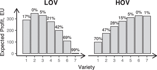
The first factor that we consider is the optimal variety (i.e., the size of the expected profit-maximizing assortment), which has two levels: the high optimal variety (HOV) condition and the low optimal variety (LOV) condition. Under the HOV condition, the optimal assortment consists of six products (i.e., ), and under the LOV condition, the optimal assortment consists of two products (i.e., ). Practically, we obtain the two conditions by varying the popularity index of the outside option ( in LOV and in HOV) and the fixed operational cost ( experimental units (EU) in LOV and EU in HOV). The profit margin for each product is EU, and the market size is λ = 1,000 potential consumers in all treatments of the experiment.
The reason that we chose these values of the popularity indices and the cost parameter K is to enable manipulation of the optimal variety factor as described. Specifically, we needed sufficient variability in the expected profit outcome, with the optimal variety falling below half of the size of the choice set for LOV and above for HOV, avoiding extreme solutions of variety 0 (empty set), 1 (no variety), or n (largest possible assortment). To meet these criteria, we made the top two products’ popularity indices nearly identical, whereas the least popular product’s index was significantly lower than that of the second-least popular product.
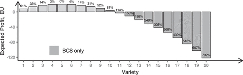
Additionally, we wanted the sequence of indices to appear intuitive and “natural” to participants, avoiding suspicious erratic gaps that could suggest specific experimenter’s demand. Therefore, we adopted a sequence resembling a square root function and finalized the values through trial and error. The resulting values of expected profits from the popular assortments of different sizes are shown in Figure 1. The labels in Figure 1 indicate the optimality gap (in percentage) that each assortment corresponds to, which is calculated as the difference between the expected profit of the assortment and that of the optimal assortment divided by the expected profit of the optimal assortment.
4.1.2. Decision Support Factor.
Our second factor in Experiment 1 pertains to the effect of the analytical decision support tools on the performance of assortment planners. We call this factor decision support information and consider three levels: no decision support information (NS), probabilities of buying (PB), and expected profit.
The baseline condition is NS, where decision makers can see only the problem parameters (i.e., the market size, profit margin, product popularity indices, popularity index of the outside option, and cost parameter) and at the end of each round, the demand realizations along with realized profits or losses. Under the PB condition, decision makers have all of the baseline condition information plus some intermediate calculations; as they click to select products in their assortment, the screen automatically displays the “chance of buying” (i.e., , the probability of choosing product from (1)) for each product in the currently selected assortment. Finally, the EP condition has the most advanced decision support information; decision makers see the baseline condition information along with the expected revenue for each product and the expected profit from the currently selected assortment. This information is automatically generated and updated as the assortment is changed. Importantly, in all three decision support information conditions, subjects have all of the necessary information to obtain these exact expected profit values themselves.
Note that in the experiment, we used the terms “average revenue” and “average profits,” which we believe, resonate better with subjects. The decision screens for all three decision support information conditions can be found in Online Appendix EC.6.
To summarize, within Experiment 1, we use a 2 (optimal variety) 3 (decision support information) full factorial design for a total of six treatments. We use a between-subject design; each subject participates only in one experiment and is exposed only to one treatment. Table 1 summarizes the key parameters of the design for Experiment 1.
|

Table 1. Comparison of Experimental Setups for Experiments 1 and 2
| Experiment | Experiment 1 | Experiment 2 |
|---|---|---|
| Choice set size | 7 | 7 (SCS) or 20 (BCS) |
| Optimal variety | 2 (LOV) or 6 (HOV) | 5 |
| Default assortment | All unchecked | All unchecked or all prechecked |
| Decision supports | NS, PB, or EP | NS and then PB′a |
| Product listing | Alphabetical | By popularity |
Note. BCS, big choice set; SCS, small choice set.
aSubjects have the option to see purchase probabilities.
4.2. Experiment Implementation
We implemented our experiment in a web application on a SoPHIE, an open source platform for conducting online experiments, via its cloud-hosted version maintained by SoPHIELabs GmbH. For Experiment 1, we recruited the subjects through the Amazon Mechanical Turk from March to May 2017, where the invitation to participate in our experiment was listed among other human intelligence tasks.
Before starting the experiment, the subjects downloaded the instructions and passed a pre-experiment quiz by answering several open-ended questions meant to ensure their understanding of the problem setup. The questions required solving a two-product version of the assortment problem: calculating the purchase probabilities, the costs, and the profits for some of the possible assortments. The subjects were not allowed to proceed until they entered the correct numbers.
After that, the subjects selected assortments for 25 rounds as described in the previous section, and they observed the revenue and profit realizations after each round. They could see the full history of their past decisions and profit realizations in a history table. Although there was no visible timer set for each period, the total experiment duration was limited to one hour to prevent subjects from seeking outside help; no subject ran out of time.
At the end of the experiment, the total profit earned by a subject across all 25 periods was converted from experimental units to U.S. dollars (USD) at the rate 1,000 EU to one USD. The resulting amount, which was inflated with a one USD fixed participation fee, was paid as a “worker’s bonus” through the Amazon mTurk system.
4.3. Experiment 1 Results
In total, 88 human subjects participated in Experiment 1; the per-treatment breakdown is given in Table 2. On average, it took a subject about 20 minutes to complete the experiment, with more than half this time spent on reading the instructions and completing the pre-experiment quiz. The average payment received by a subject, including the 1 USD fixed participation fee, was 8.75 USD with a standard deviation of 1.18 USD.
|
Table 2. Number of Subjects per Treatment in Experiment 1
| Low optimal variety | High optimal variety | Total | |
|---|---|---|---|
| No support | 12 | 12 | 24 |
| Probabilities of buying | 21 | 15 | 36 |
| Expected profit | 12 | 16 | 28 |
| Total | 45 | 43 | 88 |
4.3.1. Biases in Variety Choices.
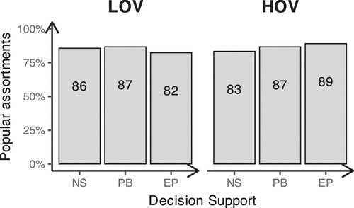
Recall that the main property of our market demand model is that the optimal solution is always found among the popular sets. As shown in Figure 2, subjects in Experiment 1 predominantly focused on popular sets. This observation suggests that this property of the problem is intuitive to the subjects. In all of our subsequent analyses, we include the observations where subjects picked nonpopular assortments. In Online Appendix EC.2, we repeat these analyses excluding the nonpopular set choices and find that all of the reported effects remain directionally identical, confirming the robustness of our results.
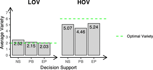
We hypothesized that subjects may offer too few or too many products, exhibiting a mean-anchoring bias; that is, the midpoint of the choice set acts as a reference point. As we see in Figure 3, in all decision support conditions, the average variety per subject is below the optimal level of six in the HOV condition and above the optimal level of two in the LOV condition, supporting our hypothesis of a mean-anchoring bias.
To confirm these observations statistically, we employ a directional asymmetry approach (Coakley and Heise 1996) to analyze subjects’ deviations from the optimal variety. This approach is chosen for its robustness, which is important given our setup, where there are more ways to deviate from the optimal variety toward the midpoint of the choice set than away from it. Testing for the difference in means in such a scenario risks overweighting deviations toward the midpoint.
We break down the subjects’ variety choices into the following three categories: (i) no deviation, in which the size of the chosen assortment was equal to the optimal variety (but the chosen assortment is not necessarily the expected profit-maximizing assortment as the included products may differ); (ii) too small, in which the size of the chosen assortment was smaller than the optimal variety; and (iii) too large, in which the size of the chosen assortment was larger than the optimal variety. Note that in this classification, we do not distinguish between popular and nonpopular assortments as defined in Section 2.2. If the midpoint serves as an anchoring point, we expect to see a higher occurrence of too large assortments when the optimal variety is below the midpoint (LOV treatment) compared with when it is above the midpoint (HOV treatment) and vice versa for too small assortments, and this is what we are testing for.
Table 3 shows the pair-wise comparisons of the average number of too small and too large deviations per subject and the corresponding Mann–Whitney U test p-values. The differences are statistically significant everywhere except for too large assortments in the EP condition (this exception can be attributed to the LOV × EP treatment, where only 11% of all chosen assortments deviated from the optimal variety of 2 (an average of 2.75 in 25 rounds per subject), and of the 12 subjects in that treatment, 5 always chose the optimal variety). Therefore, we conclude that subjects’ decisions are affected by a mean-anchoring bias.
|
Table 3. Average Numbers of Too Small and Too Large Deviations per Subject in Experiment 1 (of 25 Periods)
| Too small | Too large | |||||
|---|---|---|---|---|---|---|
| LOV | HOV | p-value | LOV | HOV | p-value | |
| NS | 1.33 | 12.50 | <0.001*** | 9.33 | 2.83 | 0.049** |
| PB | 1.33 | 16.67 | <0.001*** | 4.00 | 2.80 | 0.015** |
| EP | 1.08 | 9.25 | 0.002*** | 1.67 | 2.31 | 0.874 |
4.3.2. Effect of the Decision Support Condition.
To compare subjects’ overall performance across decision support conditions, we use the optimality gap, which is defined as the percentage by which the expected profit of a subject’s chosen assortment falls short of the expected profit from the optimal assortment in the corresponding treatment. For example, in the LOV condition, the optimal assortment yields an expected profit of 347 EU per period. If in period 2, a subject selects assortment , which yields an expected profit of 329 EU, their optimality gap is calculated as . Although the actual payoff observed by the subject is likely different from 329 as it depends on the realized product demands, we argue that using the expected profit as a basis for the performance metric is better as it is stripped from the “luck” dimension.
Figure 4 shows the average optimality gap per subject over the 25 periods. Within the LOV condition, we observe that, as expected, more advanced decision support information is associated with a smaller optimality gap—that is, improved performance. However, within the HOV condition, the optimality gap in the PB condition is higher than that in the NS condition. This is unexpected because the subjects in the PB condition received additional information beyond what was available in the NS condition—specifically, the purchase probabilities (termed “chances of buying”) for each product in any considered assortment. Calculating those probabilities is arguably the less intuitive step on the way to calculating expected profit. With this information provided, subjects were left with a simple linear calculation: summing up the “chances of buying,” multiplying the result by 1,000, and subtracting the fixed cost . These calculations were explained to the subjects in the experiment instructions, and their understanding was tested with a two-product problem during a pre-experimental quiz.
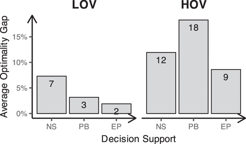
In the LOV condition, where the optimal assortment has only two products, fewer numbers needed to be added to get to the optimal assortment, and as Figure 4 shows, overall performance was better in that condition compared with HOV. In contrast, in the HOV condition, where the optimal assortment has six products, many more calculations involving the PB information were needed to reach the optimal assortment.
To assess statistical significance while accounting for multiple comparisons, we conducted a two-way analysis of variance (ANOVA) on the average optimality gap. Among the two factors—optimal variety and decision support information—only optimal variety is statistically significant (p < 0.001). The effect of decision support information (p = 0.401) and its interaction with optimal variety (p = 0.212) are not statistically significant. Nevertheless, we cannot rule out the possibility that the PB information negatively affected subjects’ performance in the HOV condition. We observe in the data that average performance in the PB × HOV treatment stays consistently worse than that of NS × HOV throughout the experiment, and panel regression results suggest a statistically significant improvement in PB in the LOV condition but an adverse effect in HOV (see Table EC.1 in the Online Appendix). Although we interpret the panel regression results with caution because of concerns about robustness, these patterns motivate additional investigation.
To investigate this puzzling finding, we analyzed the subjects’ clicks. In Experiment 1, we recorded which product boxes subjects were checking and unchecking as well as the timing of these events. These data suggest that subjects in the PB condition did not fully utilize the additional information; compared with the EP decision support, they make fewer clicks, and therefore, they see the purchase probabilities for relatively few assortments (despite choosing, on average, larger assortments than in EP in the LOV condition). We provide further analysis of the clickstream data in Online Appendix EC.3.
We suspect that in the LOV condition, the subjects tried to sum up the displayed probabilities and stopped adding products once the increase of the total exceeded the fixed cost K, which occurred after the second-most popular product. In contrast, in the HOV condition, having to add up six or seven numbers may have been cognitively taxing or discouraging. As a result, most subjects may have abandoned a systematic approach and instead, relied on heuristics or guesses, which led to worse outcomes. In other words, subjects may have felt overwhelmed by the long calculation process using the PB information in the HOV treatment, which would explain their worse performance compared with NS.
We also consider additional explanations for these puzzling observations (specifically, the salience of the cannibalization effect), which we describe and investigate in Experiment 2. As discussed later, this latter explanation was ultimately not supported by the data.
5. Experiment 2
5.1. Design and Procedure
We designed Experiment 2 to check the robustness of our findings from Experiment 1 by manipulating a different set of problem parameters and look deeper into some of the observed phenomena.
5.1.1. Default Assortment Factor.
In Experiment 1, we observe that subjects mostly choose popular assortments as the theory would suggest. Variety wise, they are more likely to choose too small assortments rather than too large assortments when the optimal variety is more than half of the size of the choice set (HOV condition), and they are more likely to choose too large assortments rather than too small assortments when the optimal variety is less than half of the size of the choice set (LOV condition), although this mean-anchoring bias appears to be weaker than in the HOV condition.
There is again a possible parallel with the newsvendor experiments literature; a number of studies (e.g., Ho et al. 2010, Rudi and Drake 2014, Feng and Zhang 2017) report that the pull-to-center effect is stronger in conditions where the optimal stocking level is higher than expected demand (in our case, corresponding to the optimal variety being higher than half of the size of the choice set—as in the HOV treatment) than in conditions where the optimal stocking level is lower than expected demand (in our case, corresponding to the optimal variety being lower than half of the size of the choice set—as in the LOV condition). However, it should be noted that the robustness of this asymmetry is still debated (Zhang and Siemsen 2019).
Another possible explanation for why the HOV condition is associated with a stronger mean-anchoring bias (and lower profits) is that reaching the optimal assortment requires more clicks than in the LOV condition (i.e., checking six product boxes instead of only two). Subjects may become fatigued from checking the boxes or perceive the initial empty assortment as a default option, and default options are known to be anchors in human decision making (Samuelson and Zeckhauser 1988, Beggs and Graddy 2009). To examine this factor, we introduce a follow-up condition in Experiment 2, where each round begins with all boxes prechecked (Pre). We call this factor the default assortment, and we have two levels; in the Un condition, all product boxes start unchecked in each period (as in Experiment 1), and under the Pre condition, all of the product boxes start checked.
5.1.2. Relative Optimal Variety Factor.
Yet another potential concern with the Experiment 1 design is that in constructing the HOV and LOV treatments, we had to vary two numerical parameters: the fixed cost K and the popularity index of the outside option . This may raise the question of whether our approach fully adheres to the principle of “changing one factor at a time.” To address this, in Experiment 2, we implement a different method to create treatments where the optimal variety falls below or above the midpoint of the choice set. We do this by manipulating the choice set size: that is, the number of possible products that the subjects can select.
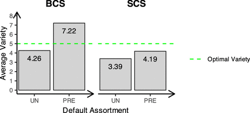
We construct two levels of this factor: the small choice set size (SCS) condition and the big choice set size (BCS) condition, both having and EU. Under the SCS condition, there are seven possible products with popularity indices , and the optimal assortment consists of the five most popular ones. The BCS condition is constructed by adding 13 more products to the choice set, which are all inferior to the initial 7 products: . In both conditions, the optimal assortment consists of the same five products. However, in the SCS condition, the optimal variety exceeds half of the size of the choice set, whereas in the BCS condition, it falls below half. Therefore, for the purpose of studying the biases in the subjects’ variety choices, the SCS condition in Experiment 2 is closest to the HOV condition in Experiment 1, and the BCS condition in Experiment 2 is closest to the LOV condition in Experiment 1.
Figure 5 shows the resulting values of the expected profits from the popular assortments along with the percentage optimality gaps. These values are the same across both conditions, but assortments exceeding a size of seven were not available in the SCS condition. Unlike in the Experiment 1 and Experiment 2 SCS condition, the subjects in the BCS condition can incur substantial losses. For example, the optimality gap for an assortment of 20 is , which means that the expected loss from such an assortment is six times greater than the expected profit from the optimal assortment. In the experiment implementation, subjects who finished the experiment with a negative total payoff ended up receiving only the minimum guaranteed payment of two USD.
Unlike in Experiment 1, the products are listed in decreasing order of their popularity indices. This is because some subjects face a large set of options, and we want to reduce the number of mistakes because of confusion. Given that the results of Experiment 1 clearly demonstrate that subjects tend to focus on popular assortments, Experiment 2 is not designed to re-evaluate this tendency.
5.1.3. Decision Support Factor.
In Experiment 1, we observed something unexpected: within the HOV condition, providing subjects with probabilities of buying information (the PB condition) led to worse performance than in the baseline condition (NS), where no decision support was given. As outlined in the previous section, one possible explanation could be that the PB information required too many calculations, which overwhelmed and confused the subjects in the HOV treatment. Another possibility is that the PB information makes the cannibalization effect more salient: directly observing purchase probabilities brings excessive attention to the fact that adding a product to the assortment decreases the probability of buying the existing ones. As a result, the subjects could become hesitant to add products to the assortment, which impacted their performance mostly in the HOV condition, where it may have led them to smaller-than-optimal assortments. This conjecture is supported by the observation that average variety in the PB condition is smaller than that in NS condition under both the HOV and LOV conditions as seen in Figure 3.
In Experiment 2, we look at the potential effect of PB information at a somewhat different angle by using the following intervention. In the first 15 periods of the experiment, all subjects operate in the NS condition from Experiment 1; that is, they receive no decision support. Then, in the last 10 periods, they operate under a condition similar to the PB condition from Experiment 1. However, unlike in Experiment 1, subjects must click a “calculate” button to view the “chances of buying” (i.e., purchase probabilities) for currently checked products. They can do so for as many assortments as they wish within the same period and then, click a separate “submit” button to finalize their assortment choice and proceed to the next period. We refer to this condition as PB′ because unlike in Experiment 1’s PB condition, probabilities are not automatically updated with each selection change.
Using a within-subject design for NS and PB′ allows us to observe how the subjects change their behavior in response to the introduction of the PB information. Further, requiring the subjects to click a button to see the decision support information allows us to track if they actually engage with it and which assortments they consider. In contrast, in Experiment 1, the probability values were displayed automatically for each currently selected assortment, making it impossible to distinguish between assortments that the subjects seriously considered and those that they briefly selected on their way to an assortment that they considered.
To summarize, within Experiment 2, we use a 2 (default assortment) 2 (relative optimal variety) full factorial design for a total of four treatments. As with Experiment 1, we use a between-subject design; however, as explained above, subjects are exposed to two different decision support systems: NS and PB′. Therefore, in that respect, we use a within-subjects design.
Table 1 summarizes the important aspects of both experiments.
5.2. Experiment Implementation
For Experiment 2, we recruited subjects through the Prolific platform (Prolific.co) from June to August 2021. Conducting the study on a different experimental platform with a distinct subject pool provides additional assurance of the robustness of our findings.
Our experiment was advertised as a study offering a performance-based bonus on top of the usual fixed participation compensation. Subjects’ profits over the 25 periods were converted at a rate of 100 EU to one USD, with a minimum payment of two USD as mandated by Prolific. Thus, if a subject’s total profit was below 200 EU, they received the minimum payment of two USD.
5.3. Experiment 2 Results
In total, 232 human subjects participated in Experiment 2 and were evenly distributed across four treatments (58 participants per treatment). The average payment received by a subject was 3.25 USD with a standard deviation of 1.08 USD.
Overall, subject performance in Experiment 2 was considerably worse than in Experiment 1, particularly in the BCS condition, as reflected in both the optimality gap and the frequency with which subjects selected popular assortments. We provide a detailed analysis of these differences in Section 5.3.3. We note that as shown in Figure 6(a), the average optimality gap in the BCS condition was abnormally high during the first three periods, suggesting a sharp learning curve. Therefore, in analyses involving means or other metrics sensitive to outliers, we exclude the first three periods for both BCS and SCS conditions. These periods are retained, however, in directional asymmetry tests.
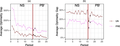
Notes. (a) BCS condition. (b) SCS condition. Panels (a) and (b) have different scales. Crosses indicate the values for periods 16 and 17, where the subjects were doing most of the engagement with the PB′ information.
5.3.1. Biases in Variety Choices.
5.3.1.1. Relative Optimal Variety Factor (Choice Set Size).
Figure 7 corresponds to Figure 3 from Experiment 1, whereas Table 4 corresponds to Table 3 from Experiment 1. Figure 8 illustrates how the average assortment size varies over time. We can clearly see that assortment sizes tend to be larger in BCS treatments (where the choice set consists of 20 products) than in the corresponding SCS treatments (where the choice set consists of 7 products). This pattern is statistically confirmed by ANOVA tests on average variety, the results of which are reported in Tables EC.4 and EC.5 in the Online Appendix.
|
Table 4. Average Numbers of Too Small and Too Large Deviations per Subject in Experiment 2 (of 25 Periods)
| Too small | Too large | |||||
|---|---|---|---|---|---|---|
| BCS | SCS | p-value | BCS | SCS | p-value | |
| Un | 14.72 | 19.91 | <0.001*** | 5.93 | 2.81 | <0.001*** |
| Pre | 7.28 | 14.43 | <0.001*** | 13.6 | 4.74 | <0.001*** |
| p-value | <0.001*** | <0.001*** | <0.001*** | 0.001*** | ||
***p < 0.01.
Note. Crosses indicate the values for periods 16 and 17, where the subjects were doing most of the engagement with the PB′ information.
Unlike in Experiment 1, when subjects start with all products unchecked (the Un condition), the variety level in both BCS and SCS conditions falls below the optimal level of five products. However, the deviation is more pronounced in the SCS condition, where the optimal variety level exceeds half of the size of the choice set.
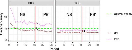
Interestingly, as we see in Figure 8, in the first few periods, the average assortment sizes in the Un × BCS condition are higher than optimal and closer to half of the choice set; that is, they are pulled to the center like in Experiment 1, but as the subjects gain experience, the average assortment size falls below the optimal level.
The Wilcoxon tests for directional asymmetry in Table 4 (p-values in columns 4 and 6) show that upward deviations from the optimal assortment size of five occur more frequently in the BCS treatments than in the SCS treatments. Conversely, downward deviations are more frequent in the SCS treatments than in the BCS treatments.
We conclude that the mean-anchoring effect that we observed in Experiment 1 is replicated in Experiment 2; subjects appear to anchor their assortment size around the midpoint of the choice set, with larger choice sets pulling variety selections upward and smaller ones pulling them downward. However, the average variety does not necessarily fall between the optimal level and half of the size of the choice set. Instead, most treatments show an overall tendency toward selecting insufficient variety.
Experiment 2 highlights how this mean-anchoring effect could be used to manipulate assortment planners’ decisions. Recall that in Experiment 2, the BCS condition is designed by adding 13 less popular products to the 7 products in the SCS condition, resulting in a choice set of size 20, and in both conditions, the optimal assortment consists of the same 5 (most popular) products. By adding a priori inferior products to the choice set, we have induced the subjects to incorporate more variety into their assortments.
5.3.1.2. Status Quo Bias.
The Wilcoxon tests reported in Table 4 (p-values in the last row) provide strong evidence that the number of clicks required to reach a solution significantly influences variety choices. Specifically, assortments that are too small occur significantly more frequently in the Un condition compared with in the Pre condition, whereas assortments that are too large occur significantly more frequently in the Pre condition than in the Un condition.
Moreover, Figures 7 and 8 clearly illustrate that assortment sizes in the Pre condition are consistently larger on average than those in the Un condition. ANOVA results confirm that this difference is highly significant overall (p < 0.001). However, Tukey’s post hoc analysis reveals that the significance of this effect depends on the choice set as the assortment size difference between the Pre and Un conditions is significant only under the BCS condition (p < 0.001) and not under the SCS condition (p = 0.168). Full ANOVA and post hoc results are reported in Tables EC.4 and EC.5 in the Online Appendix.
In the SCS condition, starting with all products prechecked (Pre condition) appears to mitigate the mean-anchoring bias compared with starting with all products unchecked (Un condition), reducing the optimality gap as we see in Figure 9—although subjects still uncheck more products than is optimal, leading to too low variety—and as we see in Figure 7.
In the BCS condition, subjects who begin with all products prechecked (Pre condition) tend to offer too much variety as seen in Figure 9. In many cases, this leads to assortments that result in negative expected profits. As a result, the average optimality gap (as seen in Figure 9) exceeds 100%, indicating that, on average, subjects incur losses.
Taken together, these findings suggest that the default starting assortment significantly influences decision making—an effect that we refer to as a status quo bias.
5.3.2. Impact of the Decision Support System.
Recall that as described in Section 5.1.3, for the first 15 periods, subjects receive no decision support as in the NS condition of Experiment 1. From period 16 onward, subjects face the condition that we label PB′, where they can click a “calculate” button to display purchase probabilities for the currently selected assortment. This differs from the PB condition of Experiment 1, where the purchase probabilities are automatically updated and displayed for any assortment that is selected.
When analyzing the subjects’ click patterns in Experiment 2, we find that all of them used the “calculate” button to compute the purchase probabilities for at least a few assortments in the first period when this functionality was introduced (period 16). However, after two or three periods, most of them stopped doing so. Interestingly, most do not settle on a particular assortment; they keep changing their solution until the very end of the experiment, which suggests that they are more influenced by the demand feedback than the PB′ information. We provide an additional discussion of the subjects’ clicking behavior from a clickstream analysis in Online Appendix EC.3.
Having established that the subjects engaged with the PB′ decision support information, we look at how it affected their performance. In Figures 6 and 8, we plot the subjects’ average optimality gap and average assortment size over time, highlighting with black crosses the values for periods 16 and 17, where the subjects were doing most of the engagement with the PB′ information.
Figure 6 suggests that the effect is again ambiguous. In the BCS condition, there is no noticeable change in the trajectory of the optimality gap. In the SCS condition, the optimality gaps drop at period 16, but by period 18, they return to pre-PB′ levels.
This pattern is particularly interesting. Although subjects’ decisions in period 16 were, on average, associated with better expected and realized profits, many quickly abandoned these strategies. A likely explanation is that those who observed lower realized profits in period 16 than in previous periods—despite the improved expected profitability—attributed this decline to the PB′ information and reverted to prior strategies. Even those who experienced performance gains may have dismissed the improvement as luck, especially if the gain was modest, or perceived their earlier underperformance as an outlier. This asymmetric attribution—crediting success to chance and failure to algorithmic decision aids—is consistent with prior research on user reactions to decision support systems (Dietvorst and Bharti 2020).
Table EC.2 in the Online Appendix presents the results of panel regressions with random subject effects using optimality gap as the dependent variable. To account for outliers, we exclude the data from the first three periods. Given the presence of multiple interaction effects, we analyze the BCS and SCS conditions separately for tractability. Because the dependent variable is lower bounded at 0%, we apply a left-censored model as in Experiment 1. We remark that the percentage of censored observations is notably lower than in Experiment 1.
The regression results suggest that introducing PB′ information has no significant effect in the BCS condition and is associated with a performance increase in the SCS condition. However, as shown in Table EC.3 in the Online Appendix, when we exclude periods 16 and 17—the two periods immediately following the introduction of PB′—the PB′ coefficient in the SCS condition becomes insignificant.
Figure 8 shows that in all four treatments, the average assortment sizes are slightly larger in period 16 compared with period 15 but revert back to pre-PB′ levels as the subjects stop relying on PB′ information. This assortment size increase goes against our previous conjecture that the PB information makes the cannibalization effect more salient because if that was the case, we would have observed a decrease in assortment sizes.
To summarize, in our experiments, a decision support tool may help or hurt subjects depending on the kind of information provided and the particular treatment. When the decision support system provides clear guidance (as in the EP condition in Experiment 1), the performance is significantly better than when no information is provided. However, information on the purchase probabilities for each product (PB in Experiment 1 and PB′ in Experiment 2) does not appear to be beneficial in most treatments. It is of particular concern that the lack of positive effect is observed in the treatments that are more challenging for the subjects, namely the HOV condition in Experiment 1 and the BCS condition in Experiment 2. Our initial conjecture that PB information biases subjects toward insufficient variety by making the cannibalization effect more salient was not supported in Experiment 2. Therefore, we incline toward our first explanation; this information is overwhelming to subjects when a large number of calculations would be required.
5.3.3. Comparison with Experiment 1.
Comparing Figure 9 with Figure 4, we see that the subjects’ performance in Experiment 2 is notably worse than that in Experiment 1. This difference could be largely because of the difference in subject pools. Recall that subjects for Experiment 1 were recruited through mTurk in 2017, whereas those for Experiment 2 were recruited through Prolific in 2021. However, we believe that it is still valuable to examine this comparison more closely as it may offer additional insight into how participants respond to different features of the experiment and may help refine our understanding of assortment planning behavior.
For a more informative comparison, we examine the two most similar treatments: Un × SCS in Experiment 2 and NS × HOV in Experiment 1. In both conditions, subjects began with all products unchecked, the choice set consisted of seven products, and the optimal variety exceeded half of the size of the choice set. When comparing performance in these cases, we find that average optimality gaps are nearly identical in the first period (24.4% in Experiment 1 NS × LOV versus 27.26% in Experiment 2 Un × SCS, Mann–Whitney U test, p = 0.5264). However, this difference becomes more pronounced when considering the 25-period averages (21.92% in Experiment 1 NS × LOV versus 25.83% in Experiment 2 Un × SCS, Mann–Whitney U test, p < 0.01). In other words, although subjects in these two treatments perform similarly at the beginning, those in the SCS condition of Experiment 2 fail to improve over time—an effect that is also evident in panel (b) of Figure 6. Panel (a) of Figure 6 suggests that subjects in the BCS condition do improve over time (likely because of learning); however, they start with particularly poor performance, and even by the end of the experiment, they do not reach the performance level observed in the SCS condition.
We observe a similar pattern when looking at the percentage of popular assortments. Comparing Figures 2 and 10 shows that in Experiment 2, the percentage of popular assortments was lower than that in Experiment 1. Moreover, unlike in Experiment 1, the percentage of popular assortments in Experiment 2 actually declined as subjects gained experience with the simulation. Here, we believe that an experimenter demand effect (when participants in an experiment alter their behavior or responses based on their perception of what the researcher wants or expects) could have played a role; because products in Experiment 2 were displayed in order of popularity (which was not the case in Experiment 1), subjects might have perceived selecting popular assortments as too simplistic to be optimal.
The fact that subjects performed worse in Experiment 2 cannot be because of the experimental parameters alone because when comparing Figures 1 and 5, we see that the optimality gap associated with a slight deviation from the optimal assortment in Experiment 2 is relatively low compared with Experiment 1.
However, it is also possible that the difference in performance is affected by a difference in the structure of the popularity indices. In Experiment 1, the gap between the seven v values is not uniform, whereas in Experiment 2, the first seven v values are one unit apart. The bigger gaps between popularity indices in Experiment 1 could have made it easier for subjects to settle on the optimal assortment. Fully understanding this possible effect would require us to run additional experiments with a different set of v values and perform those on the same subject pool, which we leave out for future research.
Yet another contributing factor to the worse performance in Experiment 2 could be the level of demand uncertainty in the simulation, which resulted from differences in parameters between Experiment 1 and Experiment 2. To construct the BCS and SCS conditions in Experiment 2 with the desired shape of the profit function, we had to set the popularity of the outside option relatively high compared with Experiment 1 (i.e., v0 = 1,500 in Experiment 2 versus 45 for LOV and 250 for HOV in Experiment 1), making it impossible for a subject to capture a large market share. Specifically, the expected market share (i.e., the probability that an individual consumer buys from the retailer, ) for the optimal assortment is 12% in Experiment 2 versus 57% and 35% in Experiment 1 for LOV and HOV, respectively. In addition to that, demand uncertainty as measured by the coefficient of variation of the revenue, which is equal to , is much higher in Experiment 2 compared with Experiment 1. As a result, profits exhibit much greater variability in Experiment 2, and in some cases, subjects experienced negative profits, even when selecting the optimal assortment. This heightened variability possibly hindered subjects’ ability to learn from feedback.
6. Conclusion
6.1. Summary of Results
The results from our experiments show that subjects who are facing the combinatorial problem of assortment planning exhibit at least two important behavioral biases: a mean-anchoring bias and a status quo bias. The mean-anchoring bias, which is similar to the pull-to-center effect observed in newsvendor experiments, means that the size of the chosen assortment is influenced by the midpoint of the choice set. This pattern is most clearly observed in Experiment 1 and in the Pre condition of Experiment 2, where the average assortment sizes tend to fall between the optimal level and the midpoint.
In the Un condition of Experiment 2, however, the average variety chosen falls below the optimal level in both SCS and BCS treatments. Still, subjects consistently choose larger assortments in BCS than in SCS, even though the optimal assortment is identical in both. This difference is consistent with the mean-anchoring bias; the BCS condition is constructed by adding 13 a priori inferior products to the SCS choice set, effectively increasing the midpoint, and this results in shifting the subjects’ variety choices upward. The overall insufficient variety in the Un condition may be explained by a status quo bias, which we describe below. Across both experiments and subject pools, the influence of the midpoint on assortment decisions remains robust and reproducible.
Importantly, Experiment 2 illustrates a practical implication of this finding; manipulating the size of the choice set can influence the decisions of assortment planners. Because our results suggest that underselection of variety is a more persistent issue (especially when subjects begin with an empty default assortment), it may be beneficial to expand the choice set, even by adding clearly inferior options. This simple intervention could nudge planners toward more complete assortments.
The status quo bias manifests itself as anchoring to the starting default assortment. In our experiments, this default is either an empty set (the Un condition) or a full set (the Pre condition), which could be either an empty assortment (no boxes prechecked) or the “full” assortment (all boxes prechecked). Our results indicate that subjects are biased toward assortments that are closer to the default assortment that they are presented with. The implication of this finding is that assortment planners might end up with larger-than-optimal assortments when tasked with “rationalizing” an existing product category than when making product selection decisions for an emerging one.
A somewhat surprising result of our experiments is the ambiguous effect of the decision support tools. Providing subjects with expected profits information (EP) is associated with better performance, but providing subjects with purchase probabilities for each product (PB) is generally not. In fact, in the HOV treatments of Experiment 1, PB is associated with lower average performance metrics compared with no decision support (NS). In Experiment 2, where we used a within-subject design to study the impact of the decision support tool, providing subjects with the purchase probabilities only seems to improve the subjects’ performance in the SCS condition and only in the first one or two periods after it is introduced. This suggests that subjects may be reluctant to rely on decision support tools when interpreting that their output requires significant effort. In practice, it means that decision support tools, like past sales visualizations, forecasts, and summary statistics, may be of little use if translating their outputs into assortment decisions is not intuitive. It is possible that they even hinder performance if the tools are perceived as too complex or opaque. As such, organizations should validate not only the accuracy but also, the usability of decision support systems before implementation.
6.2. Limitations
One limitation of our study is that the subjects are not professionals (i.e., not assortment planners or category managers in charge of curating product lines). However, previous research has shown that professional managers’ decision patterns in behavioral experiments are not significantly different from those of nonprofessionals (Bolton et al. 2012). Further, because our experiments were run on online platforms, they came with a slightly lower degree of control compared with in-person experiments. Nevertheless, it has been shown that the behavior of online recruited subjects in classic behavioral economics and operations games is very similar to the behavior observed in a traditional behavioral laboratory (Paolacci et al. 2010, Horton et al. 2011, Goodman et al. 2013, Peer et al. 2017, Lee et al. 2018).
Another limitation is the absence of a structural behavioral model. In analyzing subjects’ choices, we use dependent variables associated with the selected assortment, specifically its size, popularity, and optimality gaps. Modeling subjects’ choices for statistical analysis in our experiment presents challenges as each subject selects a subset from a set of size n (either 7 or 20), which results in mutually exclusive exhaustive alternatives—most of which were never chosen by any subject. This sparsity severely complicates estimation.
Moreover, modeling these choices would require going beyond standard random utility models (RUMs), such as the quantal response equilibrium (Goeree et al. 2005), which fails to capture the complex nature of our subjects’ data, even if applied strictly to popular assortments (see Online Appendix EC.5). Although recent literature offers RUM-based approaches for subset selection under bounded rationality (Sun et al. 2020, Tran and Mai 2024), these models typically assume that the nominal component of utility is additive in the elements of the subset. This assumption does not align with our context because of the diminishing returns inherent in the revenue structure (see (2)). We remark that the development of RUMs for combinatorial decision problems with nonadditive utilities remains an important direction for future research.
6.3. Future Research
As the first behavioral study of assortment planning, this paper opens the door to a range of future research opportunities on decision making in multiproduct contexts. Our findings offer a foundational framework for further investigation into how human planners approach assortment selection.
One interesting observation is the performance difference between Experiment 1 and Experiment 2. Although our design does not allow us to determine the exact cause, we conjecture that higher demand uncertainty in Experiment 2 driven by the relatively low market share that subjects could capture may be a contributing factor. Experiment 1 can be viewed as representing a mature product category offered by a firm with a dominant market position, whereas Experiment 2 more closely resembles a competitive market for a generic product. In such environments, poor assortment choices can be particularly costly. This highlights the need for future research on how market uncertainty affects assortment decisions.
Another important area for future investigation is the impact of decision support tools on performance. Our findings reveal mixed and context-dependent results. When the information is simple and interpretable (as in the EP condition in Experiment 1), subjects perform significantly better than those without support. However, providing subjects with purchase probability information (PB in Experiment 1 and PB′ in Experiment 2) has an ambiguous effect. In less demanding conditions (e.g., LOV in Experiment 1 and to some extent, SCS in Experiment 2), PB-type information appears to improve performance. However, in more challenging conditions, particularly the HOV condition of Experiment 1, subjects receiving PB information perform worse than those in the no support condition.
We initially hypothesized that the negative effect in more complex conditions might be because of the increased salience of cannibalization, but Experiment 2 results contradicted this explanation. At this point, we suspect that the lack of improvement that we observed was because of the complexity of the information that possibly led to confusion or disengagement.
We believe that PB information is particularly important to study as it resembles the kinds of decision support tools that managers have in practice—such as category sales forecasts or past sales statistics—rather than explicit profit estimates for specific assortments. Understanding if and why these tools may fail to help is highly important to both research and practice. Although our results provide some insight, they do not provide a general framework. Identifying the conditions under which these tools help or hinder human decision makers is a promising direction for future behavioral research.
Because we have identified behavioral biases in our research, one possible next step is to study ways to “debias” the assortment planner by providing adequate feedback and training (similar studies have been published to debias decision makers in the newsvendor problem (see Donohue et al. 2019)). By extending our setting, it should be possible to investigate the impact of decisions and phenomena related to assortment planning, such as demand censoring, the impact of ranking alternatives, learning consumer tastes, basket shopping, and combining assortment decisions with pricing and stocking decisions.
The authors thank Elena Katok and Blair Flicker for their valuable feedback and insightful suggestions throughout the development of this project. The authors are also grateful to the anonymous review team for their thoughtful comments and constructive guidance, which significantly improved the quality of this paper.
References
- (2009) Anchoring effects: Evidence from art auctions. Amer. Econom. Rev. 99(3):1027–1039.Crossref, Google Scholar
- (1985) Discrete Choice Analysis: Theory and Application to Travel Demand (MIT Press, Cambridge, MA).Google Scholar
- (2001) Reducing assortment: An attribute-based approach. J. Marketing 65(3):50–63.Crossref, Google Scholar
- (2012) Managers and students as newsvendors. Management Sci. 58(12):2225–2233.Link, Google Scholar
- (2005) Retail assortment planning in the presence of consumer search. Manufacturing Service Oper. Management 7(4):330–346.Link, Google Scholar
- (1996) Versions of the sign test in the presence of ties. Biometrics 52(4):1242–1251.Crossref, Google Scholar
- (2000) Building store loyalty through store brands. J. Marketing Res. 37(3):281–291.Crossref, Google Scholar
- (2017) How P&G and American Express are approaching AI. Harvard Bus. Rev. (March 31), https://hbr.org/2017/03/how-pg-and-american-express-are-approaching-ai.Google Scholar
- (2018) What’s your cognitive strategy? MIT Sloan Management Rev. 59(4):19–23.Google Scholar
- (2016) A “wide” variety: Effects of horizontal versus vertical display on assortment processing, perceived variety, and choice. J. Marketing Res. 53(5):682–698.Crossref, Google Scholar
- (2020) People reject algorithms in uncertain decision domains because they have diminishing sensitivity to forecasting error. Psych. Sci. 31(10):1302–1314.Crossref, Google Scholar
- (2019) The Handbook of Behavioral Operations, Wiley Series in Operations Research and Management Science (Wiley, Hoboken, NJ).Google Scholar
- (2017) Modeling strategic behavior in the competitive newsvendor problem: An experimental investigation. Production Oper. Management 26(7):1383–1398.Crossref, Google Scholar
- (2012) Which products should you stock? Harvard Bus. Rev. (November), https://hbr.org/2012/11/which-products-should-you-stock.Google Scholar
- (2006) Product variety and inventory decisions under a locational consumer choice model. Management Sci. 52(10):1528–1543.Link, Google Scholar
- (2005) Regular quantal response equilibrium. Experiment. Econom. 8(4):347–367.Crossref, Google Scholar
- (2013) Data collection in a flat world: The strengths and weaknesses of Mechanical Turk samples. J. Behav. Decision Making 26(3):213–224.Crossref, Google Scholar
- (2010) Reference dependence in multilocation newsvendor models: A structural analysis. Management Sci. 56(11):1891–1910.Link, Google Scholar
- (2011) The online laboratory: Conducting experiments in a real labor market. Experiment. Econom. 14(3):399–425.Crossref, Google Scholar
- (2000) When choice is demotivating: Can one desire too much of a good thing? J. Personality Soc. Psych. 79(6):995–1006.Crossref, Google Scholar
- (1979) Prospect theory: An analysis of decision under risk. Econometrica 47(2):263–292.Crossref, Google Scholar
- (2020) Field experiment on the profit implications of merchants’ discretionary power to override data-driven decision-making tools. Management Sci. 66(11):5182–5190.Link, Google Scholar
- (2011) Optimal and competitive assortments with endogenous pricing under hierarchical consumer choice models. Management Sci. 57(9):1546–1563.Link, Google Scholar
- (2015)
Assortment planning: Review of literature and industry practice . Agrawal N, Smith S, eds. Retail Supply Chain Management, International Series in Operations Research & Management Science, vol. 223 (Springer, Boston), 175–236.Crossref, Google Scholar - (2017) Task decomposition and newsvendor decision making. Management Sci. 63(10):3226–3245.Link, Google Scholar
- (2018) Running behavioral operations experiments using Amazon’s Mechanical Turk. Production Oper. Management 27(5):973–989.Crossref, Google Scholar
- (2014) Judgmental forecasting: Cognitive reflection and decision speed. Production Oper. Management 23(7):1146–1160.Crossref, Google Scholar
- (2010) Running experiments on Amazon Mechanical Turk. Judgment Decision Making 5(5):411–419.Crossref, Google Scholar
- (2017) Beyond the Turk: Alternative platforms for crowdsourcing behavioral research. J. Experiment. Soc. Psych. 70:153–163.Crossref, Google Scholar
- (2019) Behavioral ordering, competition and profits: An experimental investigation. Production Oper. Management 28(9):2242–2258.Crossref, Google Scholar
- (2011) Incorporating context effects into a choice model. J. Marketing Res. 48(4):767–780.Crossref, Google Scholar
- (2014) Observation bias: The impact of demand censoring on newsvendor level and adjustment behavior. Management Sci. 60(5):1334–1345.Link, Google Scholar
- (2021) How AI can help with assortment planning. Progressive Grocer 100(1):76–80.Google Scholar
- (1988) Status quo bias in decision making. J. Risk Uncertainty 1(1):7–59.Crossref, Google Scholar
- (2000) Decision bias in the newsvendor problem with a known demand distribution: Experimental evidence. Management Sci. 46(3):404–420.Link, Google Scholar
- (1989) Choice based on reasons: The case of attraction and compromise effects. J. Consumer Res. 16(2):158–174.Crossref, Google Scholar
- (1992) Choice in context: Tradeoff contrast and extremeness aversion. J. Marketing 29(3):281–295.Google Scholar
- (2020) A unified analysis for assortment planning with multi-purchase using marginal distribution models. Preprint, submitted July 23, https://dx.doi.org/10.2139/ssrn.3638783.Google Scholar
- (2024) Network-based representations and dynamic discrete choice models for multiple discrete choice analysis. Transportation Res. Part B Methodological 184:102948.Crossref, Google Scholar
- (2012) Learning consumer tastes through dynamic assortments. Oper. Res. 60(4):833–849.Link, Google Scholar
- (1999) On the relationship between inventory costs and variety benefits in retail assortments. Management Sci. 45(11):1496–1509.Link, Google Scholar
- (2019) A meta-analysis of newsvendor experiments: Revisiting the pull-to-center asymmetry. Production Oper. Management 28(1):140–156.Crossref, Google Scholar