


Time-Varying Physician Productivity and Implications for Emergency Department Modeling and Staffing
Abstract
Problem definition: Physician productivity (measured by new patients seen per hour) in emergency departments (EDs) exhibits a distinct time-varying pattern. We examine the factors contributing to this phenomenon empirically and analytically, and investigate the implications of incorporating time-varying service rates into ED modeling and physician staffing. Methodology/results: Using data from a Canadian ED, we provide empirical evidence that the “shift hour” (time elapsed since the shift started) is the most significant predictor of physician productivity. We then model the new patient pickup decisions using an optimal control framework. Assuming physicians’ objective is to maximize throughput while avoiding handoffs or overtime, the optimal policy implies adjusting pickup rates throughout a shift is a rational decision. We then investigate the impact of incorporating the time-varying physician productivity in ED modeling and staffing. Validated using data from two Canadian EDs, our simulation results demonstrate that a multiserver queueing model with shift hour–dependent service rates, despite its lower dimensionality, can accurately capture time-of-day–dependent patient waiting times, whereas models assuming constant service rates deviate significantly from observed data. Furthermore, a case study reveals that staffing plans optimized for time-varying rates outperform current practices, leading to substantial cost savings. Managerial implications: Our findings underscore the necessity of accounting for the time-varying nature of physician productivity. Hospital administrators and schedulers should incorporate this shift-hour dependency into staffing decisions to enhance resource allocation and ED operational efficiency.
Funding: This work was supported by the Research Grants Council, University Grants Committee [Grants 17501022, 17501925, CityU 11501425, and CityU 11508921].
Supplemental Material: The online appendices are available at https://doi.org/10.1287/msom.2023.0081.
1. Introduction
Emergency department (ED) overcrowding is a pressing issue facing many countries globally, significantly impacting EDs’ ability to provide timely care (Pines et al. 2011). As a result, extended patient waiting times have become extremely common in many healthcare systems around the world. To mitigate the resulting backlog and extended wait times, one must first understand the mechanics of ED flow. Because ED operations are naturally modeled as queueing systems, valid performance analysis requires a rigorous understanding of the stochastic nature of patient arrivals and service durations.
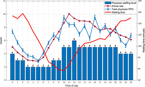
Using patient visit data from an urban tertiary hospital in Alberta, Canada, we plot the average patient arrivals per hour (demand for emergency care), physician staffing levels (ED capacity), and average waiting times (from triage to first assessment by a physician) by time of day in Figure 1. We observe that the physician staffing level in our study ED is carefully designed to match the time-varying demand. This is achieved by staggering shifts of different lengths; see a detailed description of the shift structures in Section 3. However, the outcome is less than satisfactory, because the average waiting time varies substantially over the course of the day and exceeds two hours at times.
Note. The error bars represent 95% confidence intervals.
A key determinant of patient waiting time is physicians’ speed in picking up new patients, measured by PPH—the number of new patients picked up by a physician per hour. Note that PPH is not the rate at which patients complete treatment in the ED, which is usually referred to as throughput; rather, it is the rate at which physicians pick up new patients and effectively end patient waiting in the waiting room. PPH has been used as a measure of a physician’s productivity (Joseph et al. 2018, 2021; Zaerpour et al. 2022; Niewoehner et al. 2023). Hereafter, we use physician productivity and service rate interchangeably.
We add the plot of the total physician PPH, that is, the total number of new patients seen per hour by all physicians on duty, by time of day to Figure 1. An intriguing observation is that the total physician PPH varies considerably even when the staffing level remains constant. Take the 1000-hours to 2100-hours period as an example: There are five physicians on duty during this 11-hour period, except from 1200 to 1300 hours. However, the total physician PPH ranges from 5.9 to 10.0, a 69% difference. Notably, the highest level of PPH does not coincide with the peak staffing hour, which occurs between 1200 and 1300 hours.1 In addition, the total physician PPH displays a relatively small degree of variability at any given time of day, as evidenced by the narrow 95% confidence intervals (CIs). This stability underscores the robustness of the PPH pattern. We also analyzed the total physician PPH separately for weekdays and weekends. Nevertheless, statistical tests show that the differences between the two are statistically insignificant (at the 5% level) for most hours of the day. Motivated by this system-level behavioral anomaly and the wisdom from the classical queueing theory that greater variability in service times increases waiting times, we investigate this observation further by scrutinizing the PPH at the individual physician level.
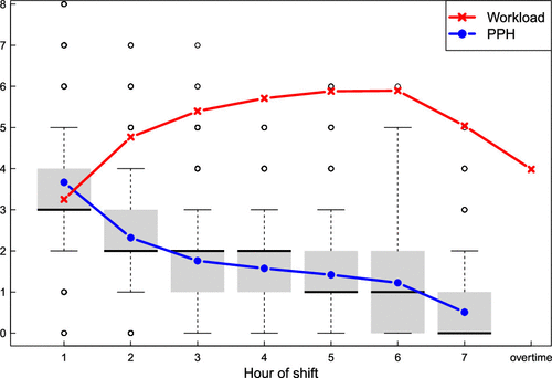
Most shifts in our study ED are seven or eight hours long. Figure 2 shows the average PPH of individual physicians by shift hour of all seven-hour shifts in the non–fast-track area from our data (see the PPH plot for eight-hour shifts in Figure A.1 in Online Appendix A). Based on the time-varying structure of PPH observed from Figure 2 and Figure A.1 in Online Appendix A, we partition a shift into three phases; within each phase, PPH exhibits distinct patterns: the start-of-shift phase (the first two hours), the end-of-shift phase (the last hour), and the middle-of-shift phase (the remaining hours of the shift). We observe that PPH decreases exponentially during the start-of-shift phase—from 3.6 in the first hour to 1.94 in the third hour (a 46% drop) in Figure 2; then, it plateaus during the middle-of-shift phase; after which, it drops to near zero in the end-of-shift phase. The pattern becomes even more pronounced for seven- and eight-hour shifts using half an hour as the time resolution (see Figure A.2 in Online Appendix A). We observe a similar pattern when we further plot the PPH for each individual physician or a specific type of shift. Comparable structures have also been reported in the emergency medicine literature using data from U.S. hospitals (Joseph et al. 2018, 2021).
Note. Physician workload refers to all patients under a physician’s care at any given time, which is also called the multitasking level (KC 2013).
Physician-level PPH dictates the aggregate service speed of the ED, directly influencing system-level performance metrics such as patient waiting times and throughput. Despite its importance, the time-varying nature of physician productivity has not been investigated in depth. Most prior studies analyze ED performance under the assumption of constant service rates, overlooking the dynamic nature of physician productivity throughout a shift (Ingolfsson et al. 2002, Savage et al. 2015, Wang et al. 2022). To address this gap, we aim to identify the factors influencing physician productivity and assess the operational implications of these factors. We specifically address two questions. (i) What factors effectively predict time-varying physician PPH? (ii) What is the impact of incorporating time-varying service rates into ED modeling and physician staffing?
To address the research questions, we conduct (i) an empirical study to establish the time—varying pattern; (ii) an optimal control model to provide a behavioral explanation for this pattern; and (iii) a simulation–based queueing model—parameterized using the empirical results from (i)—to demonstrate the value of our findings. We believe these complementary approaches together provide an integrated understanding of time-varying physician productivity and its implications for ED operations.
Our study makes the following contributions to the operations management literature on EDs. First, we provide empirical evidence that establishes the time-varying physician productivity. Using detailed operational data from Canadian EDs spanning seven months, we find that physician productivity follows a highly consistent pattern across shifts, physicians, and time periods. Our regression results in Section 3 further show that, although physician workload, ED congestion level, and other operational factors all correlate with physician productivity, shift hour is the most important predictor of physician productivity.
To further investigate the observed time-varying pattern, we develop an optimal control framework. We model the physician’s objective as maximizing throughput (completed treatments) while minimizing patient handoffs (transfer of care) or physician overtime. By analyzing the decision to pick up new patients within a finite shift, we derive closed-form expressions for the optimal time-varying PPH. Our results imply that physicians acting to avoid handoffs or overtime would exhibit service rate adjustments similar to those observed in the data. The alignment between the theoretical PPH derived from our model and the empirical data suggests a plausible mechanism for the time-varying structure: (i) The exponential decay during the start-of-shift phase is consistent with the dynamics of physician multitasking, and (ii) the sharp drop in the end-of-shift phase aligns with behavior aimed at handoff and overtime avoidance. Furthermore, our analytical results indicate that allocating additional resources to test centers may not only enhance test turnaround times but also potentially facilitate higher patient pickup rates by mitigating concerns regarding overtime and handoffs.
Finally, we investigate the practical implications of incorporating the time-varying physician productivity into ED modeling and physician staffing. We model the ED as a multiserver queue with nonstationary Poisson arrivals and exponential service times with time-varying rates. Simulation results demonstrate that this model accurately captures time-of-day–dependent performance metrics, closely matching data from two Canadian EDs. In contrast, simulations ignoring these dynamics (i.e., assuming constant rates) deviate significantly from observed reality. Furthermore, a case study reveals that staffing plans optimized under our time-varying framework outperform current schedules. Conversely, when the time-varying service rate is ignored and a constant service rate is assumed (which is the prevalent practice), the staffing plans generated using the same algorithm perform even worse than the status quo. These results highlight the practical risks of ignoring time-varying productivity in ED modeling and staffing decisions.
The remainder of this paper is organized as follows. We begin with a review of relevant literature in Section 2. Then, Section 3 describes ED operations and presents our exploratory analysis. In Section 4, we develop an optimal control model that provides a behavioral rationale for these observed patterns. We then investigate the impact of time-varying service rates on ED modeling in Section 5 and apply this framework to physician staffing optimization in Section 6. Finally, Section 7 concludes with insights and directions for future research. Proofs and supplementary results are provided in the Online Appendices.
2. Literature
Recent years have seen wide applications of operations research/management tools to improve healthcare access and reduce costs (see Saghafian et al. (2015) and Dai and Tayur (2020) for an overview). Our work aims to better understand the decision making of ED physicians underlying the time-varying productivity and thus is relevant to studies of healthcare workers’ behavioral issues. Evidence has shown that healthcare workers adjust service rates when faced with a heavy workload (Kc and Terwiesch 2009, Ding et al. 2024), high level of multitasking (Kc 2013), and overcrowded systems (Armony et al. 2015, Batt and Terwiesch 2016, Berry Jaeker and Tucker 2016). Physicians may also adapt patient prioritization behavior (Ding et al. 2019, Li et al. 2023), admission decisions (Freeman et al. 2016, Kim et al. 2020), and routing decisions (Freeman et al. 2021) to the level of system congestion. Many studies have investigated other behavioral factors and mechanisms in healthcare settings. Interested readers are referred to Kc et al. (2020) and Cho et al. (2019) for overviews on this topic.
Among them, studies that explore physicians’ behavior related to shifts are particularly relevant to our study. Batt et al. (2019) study the rate at which physicians complete patient treatments in EDs and find that the rate is lowest early in the shift and highest toward the end of shift. Chan (2018) finds that ED physicians are less likely to accept new patients and tend to speed up the treatment of existing patients near the end of shift. Deo and Jain (2019) examine the change in system speed using data from an outpatient department, where patient treatments must be completed before the end of the service episode (unlike EDs). The authors find that the service speed of a patient is slower at the start and progressively increases toward the end of the service episode. The differences between the studies above and our work are twofold: First, we focus on the rate of ED physicians picking up new patients within a shift (i.e., PPH). We find that PPH is the highest at the start of a shift, plateaus in the middle, and drops to its lowest approaching the end of shift. Shift hour is the most important predictor of PPH. Second, PPH is the rate that effectively ends a patient’s waiting in the waiting room. Through a data-calibrated simulation model, we demonstrate that considering the time-varying PPH helps build accurate models for ED patient flow, and models ignoring it generate outputs that deviate significantly from data, which further differentiates our study from the literature. It is worth noting that a recent study by Niewoehner et al. (2023) finds that working with familiar peers can increase ED physicians’ PPH in a shift which sheds light on the variation in PPH from an interesting organizational perspective, and Zaerpour et al. (2022) leverage the time-varying PPH to assign physicians to predetermined shifts. In contrast, our study identifies shift hour as the most important predictor of the time-varying PPH and uses an optimal control framework to understand physicians’ rationale. We then investigate the impact of incorporating time-varying PPH in ED modeling and physician staffing. Thus, both studies are relevant to ours but different in research methodologies and objectives.
Methodology-wise, we use the optimal control framework to model physician decision making in EDs. Hence, works that use fluid models to study healthcare systems are relevant to ours. Hu et al. (2022) use an optimal control framework to study decisions on allocating resources for proactive care when considering patient condition deterioration. Optimal scheduling policies are obtained when the system is (i) in a normal state of operation and (ii) under a random shock. Chan et al. (2021) study the dynamic assignment of nurses in EDs at the beginning of discrete shifts by a fluid control model. The authors obtain insights on the structure of “good” policies and use simulation to show that the proposed heuristics on nurse reassignment can significantly reduce the system cost compared with without reassignment. Whitt and Zhang (2017) propose an infinite-server queueing model of the ED with a time-varying arrival process, where the length of stay is used as the patient service time. Simulation results show the importance of considering the time-dependent nature of the service time, which aligns with the insights of our study. In contrast to the infinite-server model in Whitt and Zhang (2017), our model explicitly accounts for the time-dependent physician staffing level, which can support physician scheduling (as shown by the case study in Section 6).
Finally, we note the emergency medicine community has also observed a time-varying pattern of physician productivity levels. Joseph et al. (2018) find that estimating physician productivity as a simple average substantially misestimates physicians’ capacity and suggest that the time-varying pattern should be factored into physician staffing. Joseph et al. (2021) find that a decrease in PPH does not reflect a decreasing workload. These studies differ from ours in both the study objectives and framework.
3. Exploratory Study of Physician Productivity
To investigate the factors associated with time-varying productivity, we first establish the context of the ED workflow. We then introduce the data and variables. Finally, we present our empirical results and conclude with a brief discussion on possible mechanisms found in the literature.
3.1. ED Operations and Patient Care Handoff
In this section, we describe the patient flow process in the main area of the study ED, excluding the fast-track area. Our description is based on ED operations in Alberta, Canada. Although specific regional differences may exist, we believe the core features, such as the patient return-for-service process, are representative of most EDs. Patient flow in the main ED area is depicted in Figure 3.
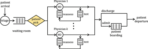
Upon arrival, patients are triaged into one of five levels, with a lower level indicating higher urgency. After triage, patients wait in the waiting room. In our study ED, the chief nurse decides which patient to move to the treatment room when an ED bed becomes available. A physician who becomes available will choose a patient from the roomed patients for initial assessment. Physicians occasionally select patients from the waiting room directly. After the initial assessment, some patients may leave the ED, whereas others may undergo diagnostic tests or medical procedures. (For simplicity, we hereafter use tests to represent all tasks performed by nonphysician staff.) Those patients will join the queue for testing (Figure 3) and return to the same physician for reassessment when the test results are ready. We refer to patients waiting to be seen in the waiting room as new patients and those waiting for reassessment as return patients. A patient may return to the same physician for service several times during an ED stay. At last, a patient departs the ED if discharged; otherwise, the patient is admitted and becomes a boarding patient, waiting in an ED bed until being transferred to an inpatient bed.
It is well known that ED physicians are multitasking (Kc 2013, Song et al. 2018, Niewoehner et al. 2023); that is, at any given time, a physician is responsible for the care of multiple patients simultaneously. Some of these patients are undergoing testing in the test queue, whereas others are waiting for reassessment (Figure 3). The number of patients under a physician’s care at any given time is referred to as the physician’s workload or this physician’s level of multitasking (Kc 2013). See Figure 2 for an illustration of the physician workload by shift hour calculated using our data.
EDs provide care 24 hours a day; however, no healthcare provider can work around the clock. As a result, shift-based scheduling is a necessity. When approaching the end of the shift, a physician must transfer the care of unfinished patients to other physicians on duty. This practice is referred to as patient handoff, which is unsafe and undesirable because it causes discontinuity of care and creates opportunities for medical errors. Handoff has been linked to up to 24% of ED malpractice claims (Cheung et al. 2010), longer patient length of stay (Epstein et al. 2010), and higher 72-hour revisit rate (Batt et al. 2019). It is suggested that physicians should “slack off” approaching the end of the shift, that is, stop signing up new patients, to avoid handoff (Chan 2018). This aligns with the practice in the U.S. ED studied by Song et al. (2015), where new patients will not be assigned to physicians during the last two hours of a physician’s shift.
3.2. Data and Variables
Physicians’ decisions to pick up new patients may be influenced by a variety of factors, such as current active workload, the need to reassess existing patients, ED congestion, and anticipated handoffs. Building on prior descriptive evidence that links productivity to shift hour, this section empirically analyzes these factors to quantify each factor’s relative contribution to within-shift productivity variance. Our goal is to identify factors with the greatest explanatory and predictive power for observed variations in productivity patterns rather than to establish causal relationships between PPH and these factors.
Our analysis is based on patient visit records and physician staffing data from the main area of our study ED, spanning January 3 to July 31, 2015. This period was selected for its stable physician staffing patterns. Figure 4 illustrates the daily physician shifts in our study ED during the study period. Each day includes 15 scheduled shifts: two fast-track shifts and the remainder in the main area. Shift lengths are six, seven, or eight hours. Shifts begin at staggered times to align physician capacity with patient demand and to prevent multiple physicians from ending shifts simultaneously, thereby facilitating smoother end-of-shift transitions.
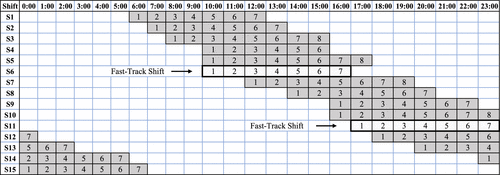
Notes. There are 15 shifts each day, with 1 six-hour shift, 10 seven-hour shifts (2 of the 10 are fast-track shifts), and 4 eight-hour shifts. The numbers in each row represent the shift hour of the corresponding shift.
We focus our analysis on the seven- and eight-hour shifts, excluding the less reliable records from six-hour shifts (flexible shifts) and the two fast-track shifts, which operate in a different area under a different model. The final data set consists of 2,475 shifts, including 1,654 seven-hour and 821 eight-hour shifts.
We aim to identify the factors that contribute to physician productivity. Hence, the response variable is the number of new patients seen by a physician during a specific hour of a shift (i.e., the PPH). Figure 2 and other descriptive results show that productivity varies significantly across shift hours. Therefore, we include a categorical variable, ShiftHour, to capture potential heterogeneity across different hours within a shift. We then include a set of control variables to account for multitasking levels, system-wide congestion, physician activities beyond new patient intake, and unobserved heterogeneity. We define Workload as the time-averaged number of active patients under the care of the focal physician during the relevant shift hour.
To control for congestion levels, we follow the literature (Zaerpour et al. 2022, Li et al. 2023) and include WaitRoomCensus (the time-averaged number of patients in the waiting room during the relevant shift hour), TreatRoomCensus (the time-averaged number of patients in ED treatment rooms, excluding boarders during the relevant shift hour), and Boarder (the time-averaged number of admitted patients who remain in the ED while awaiting an inpatient bed during the relevant shift hour). The Boarder variable specifically captures the effect of ED blocking, which has been shown to influence physician behavior (Li et al. 2023).
Physicians may also devote time to activities other than seeing new patients, such as reassessing return patients, handing patients over to other physicians, or taking handoff patients from others. We include Reassess, Handover, and HandoverTaken, which measure, respectively, the number of reassessments performed, the number of patients handed over to other physicians, and the number of patients received from other physicians during the focal hour.
To account for unobserved and temporal factors, we include several fixed effects. Physician fixed effects capture individual heterogeneity such as age, gender, experience, or baseline practice style, whereas shift fixed effects control for variation across shift types (e.g., the 0600–1300 hours versus 0700–1400 hours shifts). We also include a binary indicator, Weekend, which equals one if the shift occurs on a weekend and zero otherwise.
Summary statistics for all variables, except physician and shift fixed effects, are provided in Table 1.
|

Table 1. Summary Statistics for Variables of Interest
| Seven-hour shifts | Eight-hour shifts | |||||||||
|---|---|---|---|---|---|---|---|---|---|---|
| Variable | Mean | Standard deviation | Minimum | Maximum | 95% CI | Mean | Standard deviation | Minimum | Maximum | 95% CI |
| PPH | 1.77 | 1.42 | 0.00 | 13.00 | (1.74, 1.79) | 1.52 | 1.31 | 0.00 | 8.00 | (1.49, 1.55) |
| Workload | 6.44 | 3.76 | 0.00 | 18.00 | (6.37, 6.51) | 5.71 | 3.37 | 0.00 | 17.00 | (5.63, 5.80) |
| Reassess | 0.96 | 1.16 | 0.00 | 7.00 | (0.94, 0.98) | 0.82 | 1.06 | 0.00 | 6.00 | (0.79, 0.84) |
| HandoverTaken | 0.62 | 1.52 | 0.00 | 10.00 | (0.59, 0.65) | 0.35 | 1.11 | 0.00 | 8.00 | (0.32, 0.37) |
| Handover | 0.05 | 0.34 | 0.00 | 5.00 | (0.05, 0.06) | 0.06 | 0.38 | 0.00 | 5.00 | (0.05, 0.07) |
| WaitRoomCensus | 13.46 | 6.37 | 0.00 | 37.14 | (13.34, 13.57) | 12.91 | 5.99 | 0.34 | 37.14 | (12.77, 13.06) |
| TreatRoomCensus | 37.41 | 7.39 | 10.64 | 65.39 | (37.27, 37.54) | 40.83 | 7.03 | 16.32 | 65.39 | (40.66, 41.00) |
| Boarder | 11.38 | 4.64 | 0.92 | 33.37 | (11.29, 11.46) | 11.93 | 4.74 | 1.29 | 33.37 | (11.82, 12.05) |
| Weekend | 0.29 | 0.45 | 0.00 | 1.00 | (0.28, 0.29) | 0.29 | 0.45 | 0.00 | 1.00 | (0.28, 0.30) |
| Observations | 11,548 | 6,568 | ||||||||
| Shift Counts | 1,654 | 821 | ||||||||
Note. SD, standard deviation; CI, confidence interval.
3.3. Models and Results
Having defined the variables of interest and reported the corresponding summary statistics, we next examine how these factors are associated with physician productivity. Specifically, we estimate a series of regression models that quantify the marginal effects of key operational factors while controlling for physician- and shift-level heterogeneity. Our baseline empirical specification is given by
We begin our empirical analysis by estimating the baseline specification described in Equation (1), which includes all explanatory variables and fixed effects (Model 1). To examine the value of including different covariates in the model specification, we sequentially re-estimate the model by omitting, in turn, the physician-level activity variables (Reassess, Handover, and HandoverTaken) together with the system-level overcrowding measures (WaitRoomCensus, TreatRoomCensus, and Boarder) (Model 2); the workload measure (Workload) (Model 3); and the fixed effects associated with individual physicians (Model 4). The sequence of omitted variables follows a backward model selection approach, whereby variables are removed one at a time from the full specification. Although all these models are estimated, we report only a subset of representative results due to space constraints. Comparing the resulting values across models allows us to evaluate whether excluding these factors materially affects the explanatory power of the regression. Each set of specifications is estimated separately for seven-hour and eight-hour shifts, and the corresponding results are reported in Table 2.
|
Table 2. Estimation Results for the Effect of Various Factors on Physician Productivity
| Variable | Seven-hour-shift models | Eight-hour-shift models | ||||||
|---|---|---|---|---|---|---|---|---|
| Model 1 | Model 2 | Model 3 | Model 4 | Model 1 | Model 2 | Model 3 | Model 4 | |
| (Intercept) | 4.334*** | 3.912*** | 3.777*** | 3.471*** | 4.265*** | 4.076*** | 3.969*** | 3.411*** |
| (0.122) | (0.11) | (0.109) | (0.038) | (0.125) | (0.104) | (0.104) | (0.04) | |
| ShiftHour (base = ShiftHour1) | ||||||||
| ShiftHour2 | −1.14*** | −1.174*** | −1.319*** | −1.319*** | −0.826*** | −0.854*** | −0.991*** | −0.991*** |
| (0.04) | (0.04) | (0.036) | (0.038) | (0.049) | (0.049) | (0.047) | (0.048) | |
| ShiftHour3 | −1.597*** | −1.631*** | −1.872*** | −1.872*** | −1.381*** | −1.465*** | −1.69*** | −1.691*** |
| (0.045) | (0.045) | (0.036) | (0.038) | (0.055) | (0.054) | (0.047) | (0.048) | |
| ShiftHour4 | −1.732*** | −1.746*** | −2.032*** | −2.033*** | −1.616*** | −1.72*** | −2.022*** | −2.023*** |
| (0.048) | (0.048) | (0.036) | (0.038) | (0.061) | (0.059) | (0.047) | (0.048) | |
| ShiftHour5 | −1.894*** | −1.87*** | −2.174*** | −2.173*** | −1.808*** | −1.853*** | −2.209*** | −2.21*** |
| (0.049) | (0.049) | (0.036) | (0.038) | (0.064) | (0.063) | (0.047) | (0.048) | |
| ShiftHour6 | −2.117*** | −2.078*** | −2.381*** | −2.381*** | −1.785*** | −1.793*** | −2.16*** | −2.161*** |
| (0.049) | (0.049) | (0.037) | (0.038) | (0.065) | (0.064) | (0.047) | (0.048) | |
| ShiftHour7 | −2.827*** | −2.784*** | −3.074*** | −3.074*** | −2.073*** | −2.05*** | −2.415*** | −2.415*** |
| (0.049) | (0.048) | (0.037) | (0.038) | (0.065) | (0.064) | (0.047) | (0.048) | |
| ShiftHour8 | −2.736*** | −2.699*** | −3.037*** | −3.037*** | ||||
| (0.064) | (0.061) | (0.047) | (0.048) | |||||
| Workload | −0.036*** | −0.038*** | −0.044*** | −0.049*** | ||||
| (0.004) | (0.004) | (0.006) | (0.006) | |||||
| Reassess | −0.049*** | −0.066*** | ||||||
| (0.009) | (0.012) | |||||||
| HandoverTaken | −0.072*** | −0.059*** | ||||||
| (0.007) | (0.011) | |||||||
| Handover | −0.08** | −0.023 | ||||||
| (0.029) | (0.032) | |||||||
| WaitRoomCensus | 0.011*** | 0.015*** | ||||||
| (0.002) | (0.002) | |||||||
| TreatRoomCensus | −0.019*** | −0.008*** | ||||||
| (0.002) | (0.002) | |||||||
| Boarder | 0.016*** | −0.002 | ||||||
| (0.003) | (0.004) | |||||||
| Weekend | 0.035 | 0.076* | ||||||
| (0.023) | (0.03) | |||||||
| Physician | Yes | Yes | Yes | No | Yes | Yes | Yes | No |
| ShiftID | Yes | Yes | Yes | Yes | Yes | Yes | Yes | Yes |
| 0.478 | 0.465 | 0.461 | 0.414 | 0.506 | 0.495 | 0.49 | 0.45 | |
| Observations | 11,548 | 11,548 | 11,548 | 11,548 | 6,568 | 6,568 | 6,568 | 6,568 |
Notes. Robust standard errors are shown in the parentheses. The coefficients for the physician and shift ID fixed effect are not shown due to space limitation.
***p < 0.001; **p < 0.01; *p < 0.05.
From Table 2, we first observe that across the models for seven-hour shifts, all variables of interest included in the model have statistically significant effects on physician productivity (PPH), except for Weekend. Notably, for the eight-hour shifts, Weekend is weakly significant. Regarding model fit, removing the physician-level activity variables together with the system-level overcrowding measures results in only a marginal decrease in explanatory power, with the declining from 0.478 to 0.465 (a 2.7% drop). This indicates that, although these ED census and physician activity variables are statistically significant, the combined contribution of these variables to explaining variation in PPH is relatively small. Likewise, excluding the Workload variable further reduces the only slightly, from 0.465 to 0.461 (less than 1% drop). In contrast, the inclusion of ShiftHour factor and Shift fixed effects accounts for 41.4% of the variation in PPH. The observations for eight-hour shifts are qualitatively similar, although model fit is somewhat stronger than that of the seven-hour shifts.
The variable Workload appears to have a very marginal direct association with PPH. However, one may not infer this as evidence of negligible causal impact, because our analysis is correlational in nature. In fact, the correlation coefficient between ShiftHour and Workload is more than 0.4, suggesting that physicians’ workload tends to accumulate as the shift progresses. Consequently, this intrashift accumulation of workload may thus partially underlie the temporal productivity patterns captured by ShiftHour.
Turning to intrashift productivity dynamics, the estimated coefficients on ShiftHour reveal systematic temporal variation in PPH. For example, for the seven-hour shifts under Model 4, PPH declines sharply from Hour 1 to Hour 2 (−1.319) and from Hour 2 to Hour 3 (−0.553), remains relatively stable during the middle shifts (−0.161 from Hour 3 to 4, −0.140 from Hour 4 to 5, and −0.208 from Hour 5 to 6), and then drops considerably in the final hour (−0.693 from Hour 6 to 7).
To complement these inferential results, we further examine the relative importance of the explanatory factors from a prediction perspective (see Online Appendix B for details). In sum, the regression and prediction results underscore the dominant role of intrashift temporal dynamics, captured by ShiftHour, in shaping physician productivity. Specifically, PPH decreases significantly with shift hour over the course of a shift. Although our analysis establishes association rather than causality, the results indicate that the time-varying pattern is a robust characteristic of physician productivity.
Note that the purpose of our exploratory study is neither to establish causality nor to identify the underlying mechanisms driving the observed time-varying productivity. In particular, the time-varying PPH pattern shown in Figure 2 likely reflects the joint effects of multiple interacting factors, which makes rigorous causal identification especially challenging. Nevertheless, we believe that a brief discussion of potential mechanisms, informed by the existing literature, may be of interest to readers and helpful in guiding future research. Hence, we include a short discussion in Online Appendix C.
4. Physician Behavior Behind Time-Varying Productivity
The exploratory analysis in Section 3 establishes a robust, nonlinear pattern of physician productivity: a sharp decay at the start of the shift, a plateau in the middle, and a sharp drop near the end. Although our exploratory study identifies this pattern and links it to shift hours, it does not explain why a rational physician would adopt this pacing. In this section, we develop an optimal control framework to investigate whether a physician maximizing throughput while subject to multitasking as workload accumulates and handoff/overtime avoidance would naturally generate a productivity trajectory consistent with the empirical data. Rather than proving causality, this model serves to demonstrate that the observed PPH curve is consistent with rational behavior under ED operating constraints.
4.1. Model Description
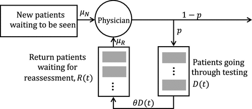
We consider a fluid model with returns to describe the patient treatment process of a single physician during a shift [0, T], where denotes the shift length. A schematic depiction of the patient flow is shown in Figure 5. We assume that there are always new patients waiting to be seen in the waiting room. Our data analysis shows that this assumption holds for most of the time in our study period. The rate of serving new patients (i.e., initial assessment) is denoted by . With probability p, a patient needs to undergo testing after assessment. Otherwise, the treatment is completed, and the patient leaves the ED. We assume that the test queue has infinitely many servers, and the mean testing time is . This infinite-server assumption aligns with Yom-Tov and Mandelbaum (2014) and Campello et al. (2016). When the test results are ready, the patient returns to the same physician for reassessment. Let and denote the number of patients in the test and reassess queues at time t, respectively. Let denote the rate at which return patients are served. After reassessment, the patient may need another test with the same probability p, independent of the number of tests that have already been performed for this patient, which implies that the total number of tests that a patient undergoes upon leaving the ED follows a geometric distribution with success probability This assumption has been adopted in the literature (Yom-Tov and Mandelbaum 2014, Campello et al. 2016, Li et al. 2023). The service and reassessment times, testing times, and return probability are assumed to be independent of the lengths of the test and reassessment queues.
Assume that a unit reward is earned when a patient’s treatment at the ED is completed. At the end of the shift, if a physician still has patients with incomplete care, the physician either goes overtime to finish the treatment or hands off these patients to other physicians, or both could happen. Note that handoffs could happen before the shift is over in practice (Batt et al. 2019). We assume that handoffs do not happen before T to simplify our model and analysis. Let denote the cost when there are x patients with incomplete care at the end of the shift: . The cost may represent the inconvenience caused by physician overtime, the time and effort required for handoff communication to transfer essential information from one physician to another, and/or the compromised quality of care due to handoffs (Cheung et al. 2010, Batt et al. 2019). It is expected that is a nondecreasing function. In this model, we do not account for the potential impact of physician fatigue on the quality of care delivered over the course of a shift. We list it as one of the future research directions in Section 7.
We further assume that return patients are prioritized over new patients, which generally aligns with the practices in our study hospitals. In our study ED, upon finishing an ongoing task, a physician logs into the ED information system through a terminal. The upper half of the screen shows the reassessment requests from the physician’s active patients, and the lower half shows the new patients waiting to be seen. The upper half is visible to this physician only, whereas the information on the lower half is available to all physicians. In general, a physician processes all the reassessment requests before signing up a new patient to limit patients’ length of stay. Physicians may also follow the shortest processing time rule because reassessment is generally faster than treating a new patient.
We believe that the primary goal of a physician is to treat as many patients as possible within a shift without exceeding overtime limits or resorting to excessive patient handoffs. Hence, we further assume that physicians do not idle when there are patients waiting for reassessment. However, physicians can choose not to see new patients to avoid overtime and/or handoffs, even if doing so requires idling. Let and denote the percentage of time that the physician spends on processing new and return patients at time t, respectively. The physician’s objective is to maximize the total net reward by controlling and . This problem can be formulated using the optimal control framework as follows:
The constraints on and , respectively, describe the dynamics of the test and reassessment queues; implies that the total percentage of time spent on initial assessment and reassessment should not exceed 100% at any time; and captures that physicians do not idle when there are return patients waiting. Specifically, is an indicator function that equals one if and zero otherwise. This constraint further implies that when , that is, there are return patients waiting for reassessment, then , that is, the physician should only focus on reassessing return patients. In other words, return patients are prioritized over new patients. The initial conditions and imply that a physician at the beginning of a shift has patients in the test queue and patients waiting for reassessment, both of which are handoff patients from other physicians.
4.2. Optimal Policy
We solve the optimal control problem (2) by applying the Pontryagin’s maximum principle. We consider three cases: (i) (ii) and (iii) In the main text, we present the results for Case (i). We focus on the first case because, in general, return patients who are waiting for reassessment will not be handed off to other physicians. The focal physician usually goes overtime to finish the reassessment of return patients in our study hospital. In fact, we do not observe any patients waiting for reassessment being handed off in our data (i.e., ). Physicians tend to avoid excessive patient handoffs. We observe from our data that the number of handoffs taken by any physician at the beginning of a shift is less than or equal to six for 97.7% of the shifts ( in our data).2 Hence, Case (i) is the most relevant case. Nevertheless, we study the optimal policies for Cases (ii) and (iii) for mathematical completeness. The optimal controls for Cases (ii) and (iii) have the same threshold structure as that of Case (i) despite the solutions being more complicated. The results for Cases (ii) and (iii) and proofs for all three cases are deferred to Online Appendix D.
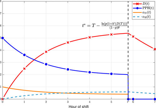
Assume that and is an increasing differentiable function. Then, the optimal control for the optimal control problem defined in (2) is of threshold type. More specifically, there exists an optimal switching time such that if ; if Furthermore, under the optimal policy, for all , where
Theorem 1 completely characterizes the optimal policy for Problem (2) under Case (i). The optimal policy implies that there exists an optimal switching time such that (i) when the shift hour is before the physician is always busy serving patients (), and priority is given to return patients over new patients; and (ii) when the shift hour exceeds it is optimal for the physician to stop signing up new patients and focus on serving return patients—even if the physician has to stay idle—to reduce the chance of overtime and patient handoffs. In fact, the proof of Theorem 1 does not require to be increasing. However, if is decreasing, it is easy to see from the expression of in (5) that . In other words, it is optimal to serve new patients at any time in the shift if more handoffs lead to lower costs, which is trivial but unrealistic and less interesting. A numerical illustration of the optimal controls is shown in Figure 6.
Note. The optimal switching time .
Assume that and The optimal switching time has a closed-form expression as follows:
Moreover, is nondecreasing in and nonincreasing in p when is a linear function.
When the cost function is linear, that is, is a constant, the expression of in (5) shows that it does not depend on and —measures of physicians’ speed in treating patients. This insight provides a justification for setting a common switching time for all physicians—despite being aware of the heterogeneity in physician speeds—when each handoff patient is perceived to contribute the same cost and the test probability p only depends on patient clinical requirements. The common switching time has been observed in practice; for example, physicians can choose not to see new patients during the last hour of a shift in our study ED, and new patients will not be assigned to physicians during the last two hours of a physician’s shift in the California ED studied by Song et al. (2015). Moreover, the monotonicity of implies that the optimal switching time is greater for bigger and/or smaller p. In other words, faster test turnaround times or a smaller likelihood of requiring additional tests allow physicians to continue seeing new patients further into a scheduled shift, rather than having to stop earlier. A key insight for hospital management is that allocating additional resources to test centers not only enhances test turnaround times but also encourages physicians to attend to more new patients due to reduced concerns about overtime and/or patient handoffs.
Assume that and
The optimal control is nonincreasing in and nondecreasing in for Moreover, decreases with for
Proposition 2 shows that, when is sufficiently small, the optimal percentage of time the physician spends on new patients increases with and decreases with and . When the chance of requiring reassessment remains unchanged, the physician will spend less time on reassessment if the reassessment can be performed faster. As a result, the physician will spend more time treating new patients. On the other hand, when physicians can treat new patients faster or the test turnaround time is shorter, more time will be spent reassessing return patients and less time treating new patients. However, this does not necessarily mean that the total physician time spent on new patients is less as the switching time increases with (shown in Proposition 1); that is, with a shorter test turnaround time, physicians continue seeing new patients and stop at a later stage of a shift.
4.3. Time-Varying Physician Productivity
Let PPH denote a physician’s productivity rate, that is, the rate of assessing new patients. Then, we have . Theorem 1 gives the following results immediately.
Assume that and Under the optimal policy for Problem (2), we have
The expressions of PPH in (6) and (7) show that a physician’s productivity within a shift is time varying. A numerical illustration of PPH is shown in Figure 6. The fact that PPH is an exponential function of the shift hour with a negative exponent explains the exponential decay of a physician’s productivity during the start-of-shift phase observed from data (Figure 2). Our model and results suggest that this early-shift decay in pickup rates can arise from physician multitasking: As the shift progresses, physicians must devote increasing attention to reassessment requests and follow-up care for return patients, leaving less time available to pick up new patients. As the shift moves into its middle-of-shift phase, the pickup rate approaches a plateau, an effect reflected mathematically by the diminishing effect of the exponential term in PPH as t increases (Figures 2 and 6). From a behavioral standpoint, the midshift plateau reflects a behavioral equilibrium in which physicians stabilize pickup rates to balance the time spent assessing new arrivals against re-evaluating return patients, rather than merely a mechanical artifact of the exponential specification. During the end-of-shift phase, overtime and handoff avoidance discourage physicians from signing up any new patients, thereby contributing to the end-of-shift drop in productivity. This decision is also suggested by Chan (2018) and Batt et al. (2019) and has been shown to be optimal under our model setting.
Note that the PPH observed from data in the last shift hour is small but above zero (Figure 2) because physicians occasionally sign up new patients during the last hour of a shift. Physicians worked overtime in 90% of these shifts. We should also note that PPH does not always decrease with t. In fact, the expression of PPH in (6) implies that when PPH increases with t. The intuition is that excessive handoff patients at the start of shift will take up physicians’ time, and thus, fewer new patients will be attended to. However, our data show that in more than 75.6% of the shifts, the number of handoff patients taken by a physician during the first hour of a shift is less than 2, whereas a rough estimate of the threshold for is about 1.7 using our data.
5. Impact of Time-Varying Service Rates on ED Modeling
The exploratory analysis in Section 3 establishes the pattern that physician productivity declines significantly over the course of a shift. Complementing this, the optimal control model in Section 4 provides a behavioral explanation for this pattern: If physicians are concerned about handoff or overtime avoidance, it is a rational decision to adjust service rates during the shift. Taken together, these findings suggest that the time-varying pattern is an intrinsic and robust feature of physician productivity. In this section, we evaluate the impact of incorporating time-varying service rates into ED models compared with the standard assumption of constant rates.
5.1. Queueing Model with Time-Varying Service Rates
A distinguishing feature of emergency care is that a patient may return to the same physician multiple times for service during the patient’s sojourn in the ED (Figure 3). With proper Markovian assumptions, the system dynamics can be represented by a Markov chain, where the system state is a vector that includes the number of patients waiting to be seen in the waiting room and the number of patients going through tests and waiting for reassessment for each physician. Unfortunately, the state space grows exponentially with the number of physicians on duty, which makes the model analysis both theoretically and computationally challenging. We aim to identify a model that can balance between details and tractability, model parameters that are easy to estimate, and system performances that match real data. Our goal is to model the patient waiting process (time from triage to first physician assessment) and staffing decisions; we therefore propose and calibrate an effective pickup-rate process rather than explicitly tracking the network of queues with return of ongoing patients as in Yom-Tov and Mandelbaum (2014).
Motivated by the findings in Sections 3 and 4, we model ED operations as an queueing system. This formulation captures time-varying arrivals, heterogeneous servers, and shift-hour-dependent service rates. The first represents a nonstationary Poisson arrival process with the time-dependent rate , which has been shown to be a reasonable assumption (Kim and Whitt 2014). Let denote the daily schedule of k shifts. Because of shift-based scheduling, the number of active physicians (servers) at time t, denoted by , varies according to the overlap of these scheduled shifts (Figure 1), where is a nonnegative integer. We assume that an exhaustive discipline is applied whenever the number of physicians decreases, that is, an outgoing physician will complete the service in progress before leaving (Ingolfsson et al. 2007). This is consistent with the practice in our study ED.
The represents exponentially distributed service times with time-varying rates, which can be estimated by the PPH of each of the physicians on duty at t. Note that the distribution of the service times is not a standard exponential distribution, and the cumulative distribution function of the service time for a patient picked up by physician n at time t is , where is the service rate of physician n at t. We further assume that the arrival rate is periodic with a daily cycle, and so is the physician scheduling. Hence, . We chose a daily cycle for ease of presentation. Moreover, physician shift schedules often repeat each day during a planning period in practice, which is the case in our study ED. However, our model can be extended in a straightforward manner to model schedules with different cyclic patterns, such as weekly cycles.
We assume that patients are served in a first-come-first-served (FCFS) manner, despite being aware that the patient prioritization process is highly complex and dependent on patients’ triage levels, waiting times, and even ED resource availability (Li et al. 2023). However, we expect that the queueing discipline has a stronger impact on metrics beyond first-moment information, such as the waiting time–based service levels (Ingolfsson et al. 2007), but has little impact on the average patient waiting time or queue length, especially given that the composition of patients at each triage level does not vary significantly over the course of the day (see Figure A.3 in Online Appendix A).
Finally, there may be more than one physician available to serve an arriving patient. Because physicians may be in different phases of the respective shifts and thus have heterogeneous service rates, we need to specify which physician serves the patient. We choose to route the patient to the physician with the highest service rate at the moment, which usually is the physician whose shift started most recently. However, one would reasonably expect that this assumption does not make much difference compared with routing the patient to an available physician randomly because EDs usually are critically loaded in a daily cycle. As a result, the chance that more than one physician is idling is small. Our simulation results confirm this conjecture.
In the following, we refer to our queueing model as an queue for simplicity. However, note that (i) the FCFS service rule when picking up a new patient, (ii) the exhaustive discipline when physicians become off duty, and (iii) the mechanism of routing a patient to the fastest physician when there is more than one idle physician are all parts of the specifications of our queueing model.
5.2. Simulation Setup
Next, we simulate the queue with parameters estimated using the data from our study ED (referred to as ED 1). The shift schedule at ED 1 from January to July 2015 is shown in Figure 4, including the start and end times (and thus the shift length) of each shift. We focus on the 13 shifts in the main ED area. The estimations of the arrival rates and the PPH for each shift are based on hourly resolution. The interarrival times of the nonstationary Poisson process are generated by the thinning algorithm. In the simulation, a physician immediately starts to serve patients at the shift start time. The service times are exponentially distributed with rates given by the PPH of the corresponding shift hour. An exhaustive discipline is applied at the shift end time.
Most existing studies on ED modeling and physician staffing explicitly or implicitly assume a single-stage physician service with a constant service rate (Ingolfsson et al. 2002, Savage et al. 2015, Wang et al. 2022). To examine the impact of considering the time-varying service rates in ED modeling, we reran the simulation model with the same parameter setting, except that the physician service rate is a constant, calculated using the total number of new patients seen divided by the total shift hours. Hence, the service rate of all physicians on duty at any time is determined by the staffing level alone.
We ran the simulation for five replications, each with 500 weeks, and we identified the first 200 weeks as the warm-up period. We focus on waiting room dynamics and choose three time-of-day-dependent performance metrics: (i) the average waiting time of patients who arrived in the same hour of day; (ii) the time-averaged number of patients in the waiting room (referred to as time-averaged queue length); and (iii) the average number of patients in the waiting room observed at the end of each hour (referred to as snapshot queue length). We compare the simulated time-of-day–dependent average waiting times and queue lengths with that from the data. To further demonstrate the generality and robustness of our results, we repeat the study using data from another ED (referred to as ED 2) in Alberta, Canada, during a different study period. We provide the comparison results but not the details of the second data set to avoid repetition.
5.3. Simulation Results
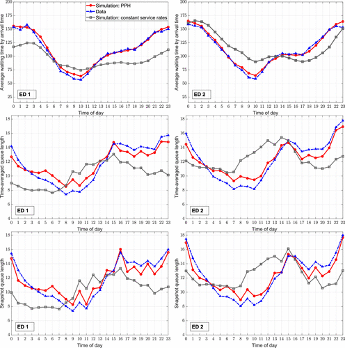
The results of comparing the simulated performance measures with the data are shown in Figure 7. We observe that the average waiting times from the simulation when the time-varying service rates (i.e., PPH) are considered nicely match those from the data from both EDs—in terms of the patterns and the magnitudes. The time-averaged and snapshot queue lengths also match the data reasonably well for both EDs; see the plots in the second and third rows of Figure 7. Furthermore, the aggregated average waiting time of all patients from ED 1 (ED 2) is 106.4 (109.5) minutes, whereas the simulated counterpart is 108.3 (110.9) minutes, which further shows the accuracy of our model.
Note. The plots on the left use data from our primary study hospital (ED 1), and those on the right use data from another Canadian hospital (ED 2).
In contrast, the simulated average waiting times and queue lengths under constant service rates deviate significantly from the data; see the gray line with squares in Figure 7. Interestingly, the variation in the simulated average waiting times between different hours of day is smaller than in the data. In other words, the simulated average waiting time curve under constant service rates is smoother. A plausible explanation is that the current physician shift schedules in both EDs were carefully designed to match the staffing level with patient demand under the assumption of constant service rates, so that the waiting times do not vary significantly over the day. However, the outcome is less than satisfactory, potentially because the scheduler did not consider the time-varying physician service rates.
To summarize, our results show that individual physicians’ behavior is crucial to the modeling of system behavior. In particular, it is important to account for the time-varying service rate (i.e., PPH) when modeling ED operations. Ignoring it is likely to fail to accurately capture the dynamics of patient flow.
Finally, we comment on the parameter estimation of the model. In principle, one simply needs to count the number of arrivals per hour and the number of initial assessments done during each hour of a shift by the physician assigned to this shift, that is, the PPH. However, one needs to be careful when dealing with real data. For example, our data cleaning identified issues including physician shift switching, system downtime due to maintenance and physician no-shows, all of which create noise in the estimation. In addition, 1.65% of patients cannot be matched with a particular shift in the data from ED 2. As a result, the total daily PPH is, on average, slightly lower than the total daily arrivals. Hence, we proportionally adjust the arrival rates downward by multiplying by 98.35%.
6. Impact of Time-Varying Service Rates on Physician Staffing
In this section, we explore the impact of incorporating time-varying service rates in physician staffing decisions. Using data from January to July 2015 for the study ED, we optimize the physician staffing by adjusting the shift start times. First, we apply algorithms that consider the shift hour–dependent service rates (i.e., PPH). Next, we apply the same algorithm but assume that the service rates are constant over the shift hours. Finally, we use our simulation model to compare the performance of the two approaches. This allows us to quantify the benefits, if any, of incorporating time-varying service rates into the physician staffing optimization.
6.1. Improving Physician Staffing: A Case Study
In our study hospital, a scheduler first determines the start and end times of each shift every six months (more or less); then, physicians are allocated to each shift following required scheduling rules. Figure 4 shows the 15 physician shifts from January to July 2015 in our study ED. Among these, S6 and S11 are fast-track shifts, and all others are dedicated to serving patients in the main ED area. Next, we adjust the start times of the 13 shifts in the main ED area (referred to as the baseline schedule hereafter) to reduce the average patient waiting time.
The shift lengths remain the same as in Figure 4. The assignment of physicians to shifts is a second-stage problem, which is not the focus of this study. Hence, we assume that the assignment is the same as in the data. Interested readers are referred to Brunner and Edenharter (2011) and Zaerpour et al. (2022) for the physician-to-shift assignment problem. In theory, the start time of each shift can be any time during the day. However, for practical relevance, we assume that physician shifts can only start at one of the 24 hours , which significantly reduces the computational complexity. Note that the adjustments in shift start times also affect the corresponding physicians’ work schedule, which may violate certain scheduling rules and make the physician-to-shift assignment infeasible. Hence, we add constraints so that the baseline schedule will not be changed dramatically. In particular, we consider three scenarios and solve the corresponding staffing optimization problem under each scenario.
Scenario 1: The physician shifts must satisfy the following constraints: (i) the two night shifts, S14 and S15, remain unchanged because night shifts often complicate physician-shift assignment; (ii) the start times of the other 11 shifts can be adjusted to be earlier or later than the baseline schedule by at most two hours; (iii) the start times of the other 11 shifts cannot be later than 2000 hours or earlier than 0600 hours; and (iv) there must be at least two physicians on duty at any time of day.
Scenario 2: The same as in Scenario 1, except that constraint (iv) is relaxed; more specifically, we require the staffing level to be at least one physician on duty at any time of day.
Scenario 3: The same as in Scenario 2, except that we relax constraints (i) and (ii) so that all 13 shifts can be adjusted to be at most three hours earlier (or later) than the start times in the baseline schedule.
Our objective is to minimize the average patient waiting time under each scenario because reducing waiting times achieves better health outcomes for patients and cost reduction for hospitals (Woodworth and Holmes 2020). One may apply simulation optimization techniques to solve the staffing problem, because there is no closed-form expression for the objective function. Indeed, we have shown that our novel simulation model can accurately capture ED waiting times. However, our attempts revealed that a commercial solver takes days to solve the optimization due to the large solution space. Hence, we propose a method that combines a local search algorithm with the uniformization method for the evaluation of each candidate schedule, and this procedure takes less than two hours for each scenario. See more details in Online Appendix E.
6.2. Results and Discussion
After solving the optimization problems under time-varying physician service rates and constant service rates, we evaluate the average patient waiting time under the baseline shift schedule and the optimized schedules for the three scenarios by simulation. Hence, a total of seven shift schedules are evaluated. We use simulation instead of uniformization so that we can construct confidence intervals. Moreover, the simulated waiting times fit the data better than the waiting times obtained from uniformization.
We run the simulation for 500 replications. For each replication, we simulate the system for 500 weeks and identify the first 200 weeks as the warm-up period which are removed from the output. We use the remaining 300 weeks to compute the average patient waiting time for each of the 500 replications.
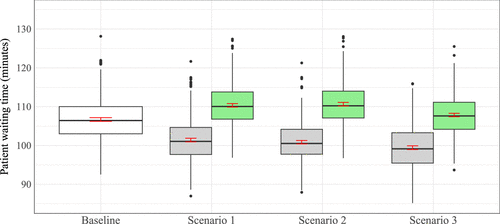
The results are shown in Table 3 and Figure 8. We first observe that, when the time-varying service rates are considered, we can achieve a better match between patient demand and ED capacity by adjusting the shift start times. As a result, the average patient waiting time can be reduced by 5.0%–6.8% compared with the baseline schedule, which is equivalent to 13.8–19.0 hours of waiting for all patients in the ED per day. (The calculation is based on an average of 156.4 patients arriving daily to the main ED area.) Figure 8 shows that the reductions over the baseline schedule are statistically significant at the 5% level.
|
Table 3. Start Times of the Optimized Physician Shift Schedules
| Scenario | Shift start times | Waiting time (min) | |||||||||||||
|---|---|---|---|---|---|---|---|---|---|---|---|---|---|---|---|
| S1 | S2 | S3 | S4 | S5 | S7 | S8 | S9 | S10 | S12 | S13 | S14 | S15 | Average | Reduction (%) | |
| Baseline (from data) | 6 | 7 | 8 | 10 | 10 | 12 | 14 | 16 | 16 | 18 | 20 | 23 | 0 | 106.7 | N/A |
| Time-varying service rates | |||||||||||||||
| Scenario 1 | 6 | 7 | 10 | 9 | 11 | 14 | 12 | 16 | 15 | 20 | 18 | 23 | 0 | 101.4 | 5.3 (5.0%) |
| Scenario 2 | 6 | 9 | 8 | 11 | 10 | 12 | 14 | 16 | 16 | 18 | 20 | 23 | 0 | 100.8 | 5.9 (5.5%) |
| Scenario 3 | 8 | 10 | 6 | 12 | 9 | 11 | 15 | 17 | 14 | 18 | 20 | 1 | 22 | 99.4 | 7.3 (6.8%) |
| Constant service rates | |||||||||||||||
| Scenario 1 | 6 | 8 | 7 | 10 | 9 | 11 | 14 | 16 | 15 | 18 | 19 | 23 | 0 | 110.3 | −3.6 (−3.4%)a |
| Scenario 2 | 7 | 8 | 7 | 10 | 9 | 11 | 15 | 16 | 15 | 17 | 20 | 23 | 0 | 110.6 | −3.9 (−3.7%) |
| Scenario 3 | 8 | 6 | 7 | 10 | 9 | 11 | 14 | 15 | 16 | 20 | 17 | 22 | 0 | 107.9 | −1.2 (−1.1%) |
Notes. The shift start times that are different from the baseline schedule are shown in bold. The last two columns show the average patient waiting time, the absolute reduction, and the percentage reduction of the optimized schedules over the baseline schedule for the time-varying service rates and the constant service rates, respectively.
aThe negative reduction represents an increase in waiting time.
Note. For each scenario, the left boxplot represents the waiting time for the optimized staffing under time-varying service rates, whereas the right boxplot represents the waiting time for the optimized staffing under constant service rates.
In contrast, when the time-varying service rates for physicians are not considered, more specifically, when we assume constant service rates over a shift, the optimized schedules perform worse than the baseline schedule. The average patient waiting time increases from 1.1% to 3.7% compared with the baseline schedule, which is equivalent to 3.1–9.4 hours of waiting for all patients in the ED per day. Figure 8 shows that the increase over the baseline schedule is statistically significant at the 5% level. Hence, we conclude that it is essential to consider the time-varying physician productivity in physician staffing decisions. Otherwise, the optimized schedules may lead to longer waiting times.
Next, we discuss the practical benefits of incorporating the time-varying service rates in physician staffing compared with using constant service rates. Take Scenario 1 for example. Table 3 shows that the average waiting time is 110.3 minutes with constant service rates, increased by 8.9 minutes from 101.4 minutes, which is the average waiting time under the optimized schedule when the time-varying service rates are considered. Woodworth and Holmes (2020) find that EDs could save the total healthcare cost approximately 2%–4% by reducing each patient’s waiting time by 10 minutes. Based on public data from a government website,3 the average cost per ED visit in Alberta, Canada, was CA$449.2 in 2015–2016. With 57,086 visits to the main ED area per year (156.4 visits/day multiplied by 365 days), the implied annual cost savings for our study hospital range from CA$456,446 to CA$912,892. One can calculate the cost differences for Scenarios 2 and 3 in Table 3 in a similar fashion. Hence, we conclude that incorporating the time-varying service rates in physician staffing can generate significant cost savings over the schedules with constant service rates. Note that these are only rough estimates, because the study by Woodworth and Holmes (2020) is based on a U.S. hospital; moreover, the distribution of the waiting time reductions among different triage levels is unclear in our results, which may affect the calculation. However, we believe that these numbers can still provide insights into the benefits of incorporating time-varying service rates in physician staffing.
7. Conclusion and Future Research
Existing ED staffing models typically assume constant physician service rates, implying that ED productivity, measured by the number of new patients that can be seen per hour, depends solely on the number of physicians on duty. Motivated by empirical observations of time-varying physician productivity patterns during shifts, we challenge this simplifying assumption by examining the underlying factors driving these variations and the resulting implications for ED modeling and staffing optimization. Our exploratory analysis reveals that shift hour is the predominant factor in explaining and predicting PPH fluctuations. Furthermore, using an optimal control framework, we demonstrate that this shift hour–dependent productivity structure is not random but a rational behavioral response if physicians are concerned about overtime/handoff avoidance. Consequently, we argue that accurate ED modeling and staffing optimization must account for the time-varying nature of physician productivity.
By overlooking the time-varying nature of physician service rates, the standard ED staffing models may fail to accurately capture the nuances of physician productivity. This can lead to suboptimal physician staffing decisions that do not fully align with the dynamic patient demands and workflow patterns in the ED. Indeed, our study demonstrates that the ED model using a constant rate fails to accurately capture the ED’s dynamics, which creates a discrepancy between the expected and actual performance of any staffing plan, undermining the effectiveness of the staffing strategy. Furthermore, our study quantifies the benefit of incorporating the time-varying service rates in physician staffing compared with using constant service rates. Our study hospital can save close to one million dollars annually by considering the time-varying physician productivity in ED physician staffing decisions. Hence, our findings call for immediate attention from hospital management and healthcare planners to incorporate the time-varying nature of physician productivity into the decision making to better match healthcare resources with patient demand.
There are a number of opportunities for future research. First, it would be of interest to extend our approach to study the time-varying nurse productivity. Nurses in the ED play a vital role in monitoring patient status, administering medications, coordinating with other healthcare providers, and so on. Hence, increasing nurse productivity is vital to improve the overall ED efficiency (Ding et al. 2024). Second, the decrease in the quality of care for patients admitted in the early stage of the shift due to physician fatigue or higher cognitive load is not captured in our model. It would be interesting to study the optimal patient pickup strategy when the quality of care and the risk caused by patient handoffs are considered. Third, it is well known that the timing of patient departures in inpatient units has an impact on ED operations (Shi et al. 2015). Hence, the stochastic fluctuations beyond the ED may also contribute to the time-varying physician productivity. It would be interesting to extend our simulation model to account for the patient flow in inpatient units to capture the complete patient journey. Finally, Green et al. (2007) highlight that the true nature of ED service times is often obscured by physician multitasking. Although modeling these interruptions explicitly is challenging, our results suggest that using PPH as an aggregate measure of service rate offers a practical and sufficiently robust alternative for ED modeling and staffing decisions. An interesting direction for future research would be to estimate physician PPH using the structured model in (7) and assess its performance based on the predicted PPH values.
The authors thank Prof. Nan Liu for early discussions on the model, as well as Department Editor Prof. Özlem Ergun, the anonymous Associate Editor, and two Reviewers for their valuable guidance and suggestions, which greatly improved the paper during the revisions.
1 One might conjecture that the variation in total physician PPH is a result of physician idling due to no patient waiting to be seen during certain periods. However, our data show that there were always new patients waiting to be seen during the high-load period (1000 hours to 2100 hours) in the study ED during our study period (January to July 2015).
2 In our data, the start time of a reassessment is available but not its end time. We use the start time of the following activity of the same physician to approximate the end time of the reassessment, which may overestimate the reassessment time, or in other words, underestimate .
3 Accessed through the Interactive Health Data Application at www.ahw.gov.ab.ca/IHDA_Retrieval/ on November 3, 2021.
References
- (2015) On patient flow in hospitals: A data-based queueing-science perspective. Stochastic Systems 5(1):146–194.Link, Google Scholar
- (2016) Early task initiation and other load-adaptive mechanisms in the emergency department. Management Sci. 63(11):3531–3551.Link, Google Scholar
- (2019) The effects of discrete work shifts on a nonterminating service system. Production Oper. Management 28(6):1528–1544.Crossref, Google Scholar
- (2016) Past the point of speeding up: The negative effects of workload saturation on efficiency and patient severity. Management Sci. 63(4):1042–1062.Link, Google Scholar
- (2011) Long term staff scheduling of physicians with different experience levels in hospitals using column generation. Health Care Management Sci. 14(2):189–202.Crossref, Google Scholar
- (2016) Queueing models of case managers. Management Sci. 63(3):882–900.Link, Google Scholar
- (2018) The efficiency of slacking off: Evidence from the emergency department. Econometrica 86(3):997–1030.Crossref, Google Scholar
- (2021) Dynamic server assignment in multiclass queues with shifts, with applications to nurse staffing in emergency departments. Oper. Res. 69(6):1936–1959.Link, Google Scholar
- (2010) Improving handoffs in the emergency department. Ann. Emergency Medicine 55(2):171–180.Crossref, Google Scholar
- (2019) Behavior aware service staffing. Production Oper. Management 28(5):1285–1304.Crossref, Google Scholar
- (2020) OM forum—Healthcare operations management: A snapshot of emerging research. Manufacturing Service Oper. Management 22(5):869–887.Link, Google Scholar
- (2019) Slow first, fast later: Temporal speed-up in service episodes of finite duration. Production Oper. Management 28(5):1061–1081.Crossref, Google Scholar
- (2019) Patient prioritization in emergency department triage systems: An empirical study of the Canadian triage and acuity scale (CTAS). Manufacturing Service Oper. Management 21(4):723–741.Link, Google Scholar
- (2024) Valuing nursing productivity in emergency departments. Manufacturing Service Oper. Management 26(4):1323–1337.Link, Google Scholar
- (2010) The impact of fragmentation of hospitalist care on length of stay. J. Hospital Medicine 5(6):335–338.Crossref, Google Scholar
- (2021) Gatekeeping, fast and slow: An empirical study of referral errors in the emergency department. Management Sci. 67(7):4209–4232.Link, Google Scholar
- (2016) Gatekeepers at work: An empirical analysis of a maternity unit. Management Sci. 63(10):3147–3167.Link, Google Scholar
- (2007) Coping with time-varying demand when setting staffing requirements for a service system. Production Oper. Management 16(1):13–39.Crossref, Google Scholar
- (2022) Optimal scheduling of proactive service with customer deterioration and improvement. Management Sci. 68(4):2533–2578.Link, Google Scholar
- (2002) Accounting for time-varying queueing effects in workforce scheduling. Eur. J. Oper. Res. 139(3):585–597.Crossref, Google Scholar
- (2007) A survey and experimental comparison of service-level-approximation methods for nonstationary queueing systems with exhaustive discipline. INFORMS J. Comput. 19(2):201–214.Link, Google Scholar
- (2021) Emergency physicians’ active patient queues over the course of a shift. Amer. J. Emergency Medicine 46:254–259.Crossref, Google Scholar
- (2018) Modelling attending physician productivity in the emergency department: A multicentre study. Emergency Medicine J. 35(5):317–322.Crossref, Google Scholar
- (2013) Does multitasking improve performance? Evidence from the emergency department. Manufacturing Service Oper. Management 16(2):168–183.Link, Google Scholar
- (2009) Impact of workload on service time and patient safety: An econometric analysis of hospital operations. Management Sci. 55(9):1486–1498.Link, Google Scholar
- (2020) Empirical research in healthcare operations: Past research, present understanding, and future opportunities. Manufacturing Service Oper. Management 22(1):73–83.Link, Google Scholar
- (2014) Are call center and hospital arrivals well modeled by nonhomogeneous Poisson processes? Manufacturing Service Oper. Management 16(3):464–480.Link, Google Scholar
- (2020) Admission control biases in hospital unit capacity management: How occupancy information hurdles and decision noise impact utilization. Management Sci. 66(11):5151–5170.Link, Google Scholar
- (2023) Who is next: Patient prioritization under emergency department blocking. Oper. Res. 71(3):821–842.Link, Google Scholar
- (2023) Physician discretion and patient pick-up: How familiarity encourages multitasking in the emergency department. Oper. Res. 71(3):958–978.Link, Google Scholar
- (2011) International perspectives on emergency department crowding. Academic Emergency Medicine 18(12):1358–1370.Crossref, Google Scholar
- (2015) Operations research/management contributions to emergency department patient flow optimization: Review and research prospects. IIE Trans. Healthcare Systems Engrg. 5(2):101–123.Crossref, Google Scholar
- (2015) Developing emergency department physician shift schedules optimized to meet patient demand. Canadian J. Emergency Medicine 17(1):3–12.Crossref, Google Scholar
- (2015) Models and insights for hospital inpatient operations: Time-dependent ED boarding time. Management Sci. 62(1):1–28.Google Scholar
- (2015) The diseconomies of queue pooling: An empirical investigation of emergency department length of stay. Management Sci. 61(12):3032–3053.Link, Google Scholar
- (2018) Closing the productivity gap: Improving worker productivity through public relative performance feedback and validation of best practices. Management Sci. 64(6):2628–2649.Link, Google Scholar
- (2022) Physician scheduling for emergency departments under time-varying demand and patient return. IEEE Trans. Automation Sci. Engrg. 20(1):553–570.Crossref, Google Scholar
- (2017) A data-driven model of an emergency department. Oper. Res. Health Care 12:1–15.Crossref, Google Scholar
- (2020) Just a minute: The effect of emergency department wait time on the cost of care. Econom. Inquiry 58(2):698–716.Crossref, Google Scholar
- (2014) Erlang-R: A time-varying queue with reentrant customers, in support of healthcare staffing. Manufacturing Service Oper. Management 16(2):283–299.Link, Google Scholar
- (2022) Scheduling of physicians with time-varying productivity levels in emergency departments. Production Oper. Management 31(2):645–667.Crossref, Google Scholar

