
Distinguishing Useful and Wasteful Slack
Abstract
The literature on organization and strategic management suggests that slack in the form of excess resources may be useful. It may, for example, serve as a buffer against environmental shocks, help decouple organizations, ease planning and implementation, support innovation, and enable effective responses to competitors. In contrast, the economic literature tends to view slack as wasteful. When the same products and services can be produced with fewer resources and slack per se is not assigned any value, slack should be eliminated. The aim of this paper is to reconcile these two perspectives. We acknowledge that slack may be both useful and wasteful. The challenge is how to separate the two. Our approach relies on the simple Pareto idea. If an organization can maintain the same levels of output and slack at lower cost, there is wasteful or nonrationalizable spending. We develop ways to measure the extent to which total spending can be rationalized and show how to statistically estimate and test the usefulness of the available slack using bootstrapping.
Funding: Financial support from Det Frie Forskningsråd [Grant 9038-00042A] is greatly appreciated.
Supplemental Material: The online appendix is available at https://doi.org/10.1287/opre.2022.2415.
1. Introduction
The idea of organizational slack in the form of excess resources has been present in the organizational and strategic management literature for many years. It has been suggested that slack may serve as a cushion against uncertainty, a buffer against environmental shocks, a means to decouple organizations and ease planning and implementation, an opportunity to respond effectively to competitors, etc.
In neoclassical economics, slack tends to be regarded as waste and should be minimized—and eliminated if at all possible. Of course, there are many economic models where some slack is optimal. The optimal resource allocation in a dynamic model may differ from the static version and involve slack. Additionally, under conditions of uncertainty, slack is prevalent, and under asymmetric information, slack may well be part of a second-best solution and serve as remuneration to an agent. Nevertheless, the general idea in economics is that when the same products and services can be produced with fewer resources and slack per se is not assigned any explicit value, slack should be eliminated.
In this paper, we accept that slack may be useful for a multiplicity of reasons and may in itself be multidimensional. We focus instead on how to distinguish useful slack from useless slack, which is the genuine waste of organizational resources.
The idea is simple; genuine, wasteful slack (inefficiency) is present when not only the same production but also, the same slack consumption is possible at less cost. We measure the wasteful slack by the extra costs that could have been saved without reducing either the production or the slack. In this way, we provide a best-case measure of the usefulness of an organization’s slack.
Specifically, we propose an approach to decompose the total cost into rationalizable and nonrationalizable costs. The rationalizable cost is the minimal cost necessary to produce the outputs plus the cost of useful slack. The nonrationalizable cost is the cost of wasteful slack (i.e., the costs that could have been avoided without reducing either the production of final outputs or the level of any type of slack).
Moreover, we show how to measure and test hypotheses about the share of rationalizable costs (SoRC), defined as
In this way, we make several important contributions. We include organizational slack in a production economic model, develop a continuous notion of the degree of rationalizable behavior, and produce methods to test hypotheses about the degree of rational behavior.
Of course, our approach also has its limitations. As will be made clear, we need data on the resources used and the products and services produced by an organization (and preferably, several other organizations as well). We also need to know factor prices or product prices in the evaluated organization, and to obtain an interesting decomposition, we need at least two inputs or two outputs.
The outline of the paper is as follows. In the next section, we discuss different notions of slack and some of the more detailed findings in the literature. In Section 3, we formalize and operationalize the rational perspective and develop the notion of the share of rationalizable cost, SoRC. In Section 4, we discuss how to test hypotheses about the SoRC. In particular, we show how to test whether an individual firm or the firms in an industry comply with a rationality hypothesis. In Section 5, we apply our approach to a real-world data set. Another application is discussed in the online appendix. Concluding remarks are given in Section 6.
2. Literature
The idea of organizational slack has been important in the organizational and strategic management literature for many years. Early on, Barnard (1938) conceptually discussed how a large inducement-contribution ratio (i.e., reward-effort ratio) could attract organizational participants and sustain their membership. March and Simon (1958) similarly used the notion of slack as a source of inducement that might lead to an inducement-contribution ratio above one (i.e., where the organization pays an employee more than would be required to retain his services). The concept was later clarified in Cyert and March (1963) as the condition where inducement in the form of income and prestige exceeds the amount required to obtain the member’s contribution. Because a manager’s salary and status are frequently associated with the size of the department, one of the more prominent slack-creating tactics used in organizations is empire building, whereby additional administrative positions and titles are created (cf. Williamson 1963).
Although many papers discuss organizational slack, it is rarely treated in anything other than conceptual terms and therefore, has not been effectively operationalized for empirical treatment. Moreover, the definitions used by different authors are not uniform. A useful overview of the slack concept is provided in Bourgeois (1981), who also, as an important contribution, discusses different operational indicators of slack based on financial data.
Bourgeois (1981, p. 30) condenses the notion as follows: “Organization slack is that cushion of actual or potential resources which allows an organization to adapt successfully to internal pressure or adjustment or to external pressure for change in policy, as well as to initiate changes in strategy with respect to the external environment.”
Hence, slack can be seen as a cushion of spare resources that prohibits an organization from collapsing in the face of a surge of activities. This dates back to Cyert and March (1963), who noted that the traditional economic ideal of zero slack is viewed by practitioners and organizational researchers as unrealistic. Organizations need “shock absorbers.”
Similarly, organizational slack helps decouple activities and reduces the need for excessive information flows in large organizations (cf., e.g., Galbraith 1973, 1974).
The last part of the Bourgeois (1981) definition is more strategically oriented. Research focusing on strategic aspects has emphasized that slack allows organizations to experiment with new strategies and innovations, eases the search for satisficing actions, and potentially lessens conflicts among divergent subunit interests.
Hence, slack can serve different purposes. There are, therefore, different types of slack and correspondingly, several possible measures of slack.
At the general level, a common typology distinguishes among available, recoverable, and potential slack resources (cf., e.g., Herold et al. 2006). Available slack (also sometimes called unabsorbed slack) represents resources that are not yet committed to specific usages. Profits can, for example, be used both to fund innovation and to increase dividend payments. Recoverable slack (sometimes called absorbed slack) is excess resources that are presently absorbed by the organization (e.g., as excessive overhead, which could be recovered through increased efficiencies if needed in a bear market for example). Potential slack represents the future possibility of accessing resources (e.g., by raising additional equity).
Focusing on slack for internal maintenance of the organization, it can help provide inducements, lower internal conflicts, and serve as a buffer facilitating coordination of different subunits. The inducement aspect can be captured by indicators such as excess dividends; low prices to retain customers; high wages to retain employees; and high income, prestige, and perks as management inducements. Conflict mitigation can be facilitated by allowing the pursuit of pet projects, lowering ROIs and increasing financial authority. Last, slack may serve as a technical buffer reducing the need for coordination and communication by introducing larger inventories, buying more equipment, etc.
Focusing instead on slack as a facilitator of strategic planning, one can measure the use of slack for innovation by new products, processes, markets, R&D budgets, etc. Slack can also reduce the time necessary to search for new satisficing solutions or team members. Moreover, slack can be used as an infusion of new uncommitted resources, which may limit the internal conflicts over reallocations.
It is clear that empirical analysis of slack may require context-specific information that is often not easily available. For several of the dimensions, interviews and questionnaires are the most likely sources of information. As an interesting alternative, Bourgeois (1981) suggests a measure of slack that is based on external financial data. Specifically, he proposes constructing a composite measure of increases in slack by examining financial accounting items. Increases in slack could be associated with increases in retained earnings, general and administrative expenses, working capital as a percentage of sales, credit rating and price-earnings ratio, decreases in dividend payouts, debt as a percentage of equity, and short-term loan interest.
Before closing this introduction to the literature, it is worthwhile to make a few more general observations. Slack may have a positive impact, as suggested by the definitions. Consistent with this perspective, Daniel et al. (2004) and others, such as Singh (1986), Bromiley (1991), Herold et al. (2006), and O’Toole and Meier (2010), have found positive associations between slack and organizational performance. Firms must have access to unallocated resources to exploit opportunities for expansion and to endure economic downturns. However, slack may also be wasteful and even harmful, as emphasized by the economic approach. Slack may not only be the result of inefficient resource allocation, but worse, it may enable managers to engage in self-serving and value-destroying activities (Jensen and Meckling 1976).
One hypothesis is, therefore, that the correlation between success and slack is positive up to an inflection point and then, negative. That is, the relationship is curvilinear following an inverted U shape as a manifestation of what Pierce and Ahuinis (2013) calls the “too-much-of-a-good-thing” effect. The inverted U-shape perspective has found empirical support in, for example, Tan and Peng (2003). Other support for this is from Tseng et al. (2007), who show that organizational slack has a curvilinear relation with a success measure such as international expansion; Bradley et al. (2011), who find that resource slack represents a double-edged sword, simultaneously fueling and hindering entrepreneurial growth; and Hvide and Moen (2010), investigating the relationship between entrepreneurs’ wealth and start-up performance.
In this paper, we suggest a novel approach to the measurement of slack. We assume that a firm values both profit and slack. A rational firm must, therefore, make trade-offs between profit and slack or between cost minimization and slack consumption. In addition, the firm must make trade-offs between different types of costly slack. We build a rational economic model of the slack selection process and examine to what extent it can rationalize observed behavior. When a full rationalization is not possible, we measure the largest share of total costs that can be rationalized by the model. We do so within a framework of traditional production economics as in, for example, Debreu (1951), Koopmans (1951), Farrell (1957), and Shephard (1970).
Methodologically, the paper is related to the “nonparametric production analysis” or “nonparametric tests of optimizing behavior” literature as Varian (1984, 1985, 1990) calls it. This approach is rooted in the theory of revealed preference of Samuelson (1947) and the work of Afriat (1972) and Hanoch and Rothschild (1972). The question is whether observed outcomes are consistent with utility optimization for some reasonable preference function.
This literature has many technical similarities to more recent productivity analysis using mathematical programming as noted in, for example, Banker and Maindiratta (1988) and Färe and Grosskopf (1995) and is not void of applications (cf., e.g., Chavas and Cox 1990, 1992, 1995). A fundamental difference is that although modern productivity analysis is mostly concerned with identifying and measuring the degree of “inefficiency/irrationality,” this paper, like the revealed preference literature, is mostly concerned with attempting to understand inefficiency as the result of rational choices. In this sense, the present paper extends the idea of rational inefficiency introduced as a dichotomic concept in Bogetoft and Hougaard (2003) and subsequently applied in Asmild et al. (2009, 2013a) and Bogetoft and Andersen (2009). The binary nature of the rational inefficiency concept, unfortunately, limits its analytical relevance. Therefore, in this paper, we focus on the degree of rational inefficiency in the form of the share of rationalizable costs, SoRC. This provides a continuous measure that seems more useful in applications than the original dichotomic notion. In practice, it is not only relevant if behavior can be rationalized (when introducing the idea that slack may be useful); it is also relevant to know if behavior can be almost rationalized and if the extra costs of deviation from rationalizable behavior are large or merely associated with a minor increase in spending.
Moreover, we extend previous rational inefficiency studies by introducing statistical tests for hypotheses about the continuous SoRC measure. This is also very important in applications. If by chance (i.e., random choice of inputs vectors), it is very easy to obtain a high level of rationalizable costs, a high SoRC score is not a strong sign of (almost) rational behavior. The likelihood of obtaining a high SoRC score depends intimately on the production technology, and it is, therefore, important to find ways to formally test the significance of an SoRC score. In this paper, we derive such tests using bootstrapping.
There have been few papers testing the rational inefficiency hypothesis. One possibility, however, is to use the Asmild et al. (2013b) approach to test for overrepresentation of observations in certain regions of the production space. Asmild et al. (2013b) rely on volumes of “production zones” (i.e., subsets of the production set) to estimate the probability that an observation falls within a prespecified production zone. Using their approach and assuming common input prices for all firms, one would expect all observations to be located close to the cost-efficient point. If more observations fall in the production zone dominated by the cost-efficient point than expected by chance alone, then this might be evidence of the rational inefficiency hypothesis. In this way, Asmild et al. (2013b) offers an interesting approach to test the dichotomic concept of rational inefficiency. Our approach uses a similar idea to test hypotheses about the continuous SoRC measure. In our case, the total cost of a given firm is known from the inputs and their prices. We can, therefore, calculate the probability of appearing rationally inefficient (SoRC = 1) as the ratio of the volume of the rationally inefficient subset of the isocost hyperplane to the volume of the technically feasible part of the isocost curve. Similarly, we can calculate the probability that SoRC is above some threshold level. We can easily implement this approach using numerical simulations. One obvious advantage of our approach is that it directly gives an estimate of the null distribution of the continuous SoRC measure. The approach of Asmild et al. (2013b) may nevertheless suggest ways to refine our approach to dispense with null assumption of a uniform distribution. Additionally, in some cases, it may be useful to rely on qhull procedures Barber et al. (1996) to calculate volumens rather than our suggestion of using numerical simulations.
An important feature of our approach is that we identify different types of slack (i.e., different levels of slack in different resources). The composition of slack is not directly observable. It is not obvious if an organization is economically inefficient because it applies too much labor or too much capital for example. To address this problem, we infer the composition by contemplating what a rational entity would do. That is, we let the benefit of the doubt regarding the usefulness of different types of slack speak in favor of the evaluated entity.
By attempting to describe the slack selection process in greater detail, we open up the black box of traditional productivity analysis. We not only note that a firm is X inefficient but also attempt to understand in which way it is inefficient. We are thereby in line with Stigler (1976), who argues against the Leibenstein (1966, 1978) concept of X inefficiency. X inefficiency means that too many inputs have been used to produce too few outputs. According to Leibenstein (1966, 1978), X inefficiency is primarily caused by the lack of motivation and knowledge. If an inefficient firm does not motivate its employees sufficiently to save inputs and expand outputs, performance may be improved by redesigning the incentive structures. If inefficiency is caused by a lack of information, performance may be increased by improving the markets for knowledge, learning, etc. Stigler (1976) suggests that “Leibenstein does not attempt to understand the allocation of ‘inefficient’ resources and hence does not see the necessity for attributing his X-inefficiency to specific inputs.” In this paper, we attempt to do exactly that; we regard slack and in particular, the allocation of slack among different inputs as the result of a rational choice made by that firm.
Another important feature of our approach is that we distinguish useful and wasteful slack. The traditional view on organizational slack as embodied in the inverted U shape is that slack first has positive consequences and later, negative effects. We do not regard slack as a one-dimensional feature. Rather, we suggest that there may be both useful and wasteful slack present simultaneously and for all levels of total slack. That is, even a relatively lean firm may have wasteful slack, and a fat organization may have purely useful slack. It is not the level of slack that matters; it is the composition of slack.
Because we allow for several possible applications of slack and because different types of both unabsorbed and absorbed slack are, therefore, of potential interest, it is not surprising that our approach also requires more data than an approach focusing on the impact of one resource on one performance dimension. Our approach ideally requires information about inputs used and product and services being produced as well as prices of the different inputs (or outputs). The approach can, however, work with more or less aggregated production data and may even rely on financial data. The multiplicity of inputs or outputs is, however, crucial because it is the composition of inputs and outputs that determines whether slack is potentially useful or wasteful.
As a final perspective, note that slack can also be viewed as the result of model misspecification. Measured waste may reflect that not all inputs or outputs are accounted for, that heterogeneous inputs and outputs are pooled, or that the assumed relationship between inputs and outputs is flawed. Uncertainty may also lead to a misspecification problem. Efficiency is commonly measured ex post and not ex ante. The ex post approach may be overly harsh, especially if organizations are operating under significant uncertainty. In this paper, we accept that model misspecifications may be present. We do not, however, forego the idea of measurement. Rather, we suggest defining other measures, including the share of total slack being potentially useful.
3. Formal Setting and Concepts
In this section, we introduce our production economic framework and discuss how to distinguish between useful rationalizable and wasteful nonrationalizable slack. Finally, we formalize our measure of the share of rationalizable costs.
3.1. Technology
We consider a firm (organization) using p inputs to produce q outputs . To simplify the exposition, in the main part of the paper, we focus on the input space and slacks in terms of excessive input consumption that we might regard as on-the-job consumption of inputs (i.e., inputs that are not used directly to produce the observed outputs). A parallel treatment with slack on the output side (i.e., with insufficient output delivery because of, e.g., on-the-job consumption of outputs (e.g., farm products) or excessive final product inventories) is certainly possible.
The technology can be described by the input requirement set
The efficient subset represents technically efficient production plans. It involves no “waste” or excessive consumption of inputs.
When the inputs have associated prices , we are traditionally interested in the (minimal) cost of producing a given output y with input prices w,
Additionally, we are interested in the associated input combinations and define the allocatively efficient inputs as the set of minimal cost input vectors able to produce y:
Production economics has traditionally focused on technically efficient production plans Xe and allocatively efficient plans . The hypothesis of this paper is that these concepts are useful but insufficient to characterize rational behavior. Nontechnically and nonallocatively efficient production plans may still be fully rational when we assign positive values to slack.
3.2. Slack
Now, consider the case where a firm has used a technically inefficient input combination . The input vector x is observable by an outside observer.
In theory, the firm may have used the procedures and techniques associated with an underlying production plan z and then added some slack in the different input dimensions, such that . Neither the underlying production plan z nor the slack vector s can be observed by an outside observer. However, we can make inferences about z and s based on x and the assumption that the firm chooses z and s rationally.
Note first that because all inputs used are accounted for in the input vector x, slack must be nonnegative. If some inputs were not accounted for (e.g., because the producing agent brought private funds into the production process), slack could be negative. If, for example, and , we obtain a slack vector . This is only possible if the producing agent brings at least one unit of the second input into the production process, and we do not account for this in x.
Second, we see that by slack being nonnegative, the underlying production plan z must weakly dominate x (i.e., the underlying production plan can be any with ).
With no further information, we cannot know exactly which plan z the firm has used as the “underlying” production plan. Along the same lines, we cannot say exactly which slack vector the firm has consumed; we know, however, having observed x that it belongs to the slack possibility set defined as
Hence, although we cannot directly observe slack, we can at least make partial inferences about the possible multidimensional slack vectors.
In addition to possibly enjoying the consumption of slack, the firm will also typically be concerned about profits or for fixed outputs y, costs . In the following, we will assume that the firm has the dual objectives of minimizing costs and maximizing slack. We do not know the relative strength of these objectives and are, therefore, unaware of the willingness to make trade-offs between lower costs and higher slack.
We can also express this by stating that the firm’s total utility is a function of cost and slack ,
To summarize, we can regard the firm’s problem as one of choosing a cost level c, an input mix x, and a slack vector s to maximize the resulting utility
Now, it is clear that a firm seeking to minimize costs and maximize slack should choose an allocatively efficient production plan as the underlying production plan . This observation is tightly related to proposition 1 in Bogetoft and Hougaard (2003). We, however, offer an alternative and more expanded proof based on contradictions and record it here as a lemma.
In an optimal solution to the firm’s problem, the firm will choose input consumption x and slack vector s such that the underlying production plan is allocatively efficient (i.e., ).
Because U(c, s) is strictly decreasing in c and c only appears in the first constraint of the firm’s problem, the first constraint must be binding (i.e., we have c = wx). We can, therefore, rewrite the firm’s problem as
Let (s, x) be a solution to this problem, and let us assume that in not allocatively efficient (i.e., ).
We will show that z not being allocatively efficient contradicts the optimality of (s, x).
To do so, let be an allocatively efficient input vector that can produce y (i.e., ). Because it is allocative efficient, it is less costly than z (i.e., we have
Now, define as
We have that is also a feasible solution to the firm’s problem because , and
However, leads to a higher objective function value than (x, s) (i.e., ) because the utility function is strictly decreasing in the first argument, and we have
The content of Lemma 1 is illustrated in Figure 1.
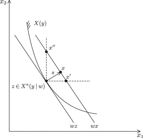
The intuition is that the firm acquires the necessary inputs to produce y in the cheapest possible way using Whatever extra spending is considered can then be divided between slack and cost reductions. To emphasize this, note that given an optimal choice of the underlying production plan, the firm’s remaining decision can be formulated as the following slack selection problem:
This shows that the choice of slack is done by trading off the extra costs in the first argument of against the extra value from slack in the second argument of .
In Figure 1, if the firm only values slack of the first input type, x1, it will choose . Likewise, the firm will choose if only slack in x2 is valuable to it. All points on the line can be fully rationalized at total cost wx by the idea that slack is valuable. They can be rationalized because they fall in the intersection of the extended cone and the isocost line wx (cf. also Lemma 2). Thus, and are the most “extreme” allocations that can be fully rationalized.
From the perspective of production theory, Lemma 1 shows that the traditional definition of allocative efficiency is useful even in the extended setting with possible values of slack that we consider here. Note that in our setting, prices reflect market conditions, and allocative efficiency focuses on adjusting production factors to market prices, which do not necessarily reflect the values of these resources inside the firm. The values to the firm are determined by both the spending and the slack that is consumed. The underlying preferences for slack, say in labor versus capital, do not affect the underlying production plan , but they do affect the actual production plan x.
Although the choice of an actual production plan x depends on the specific preferences for slack and cost (profit), we can impose simple constraints on the possible production plans that a rational firm can choose. From Lemma 1, we have that , and because we obtain . We record this in another lemma similar to corollary 1 in Bogetoft and Hougaard (2003).
In an optimal solution to the firm’s problem, the firm chooses the actual production plan as .
That is, to obtain the “optimal” slack possibility set, the firm must locate itself in a position where some point in Xa will dominate it; the exact location will, of course, depend on the firm’s specific value function U(c, s).
In summary, we can regard a firm caring about both cost and slack as taking the following steps to decide how to produce the required output vector y.
Minimal cost plan. First, given the prices w and the technology X(y), the firm identifies the inputs that are able to produce the requested outputs at the lowest possible cost.
Excess spending on slack. Next, the firm determines how much additional cost to spend on slack. Costs increase as the isocost hyperplane moves upward, and the trade-off between cost minimization and slack consumption determines how much cost the firm is willing to spend to allow for slack.
Allocation on slack types. Finally, given some cost level, , the firm decides how to trade off different types of slack by maximizing the value of slack on the segment of the isocost hyperplane that intersects (e.g., the segment to in Figure 1).
Taking this approach, we can in principle rationalize all production plans in the (translated) cone . For each point in the cone, there exists a utility function U(c, s) that is decreasing in c and increasing in s and that makes the specific point the rational choice (i.e., the solution to the firm’s problem). We say that all slack in this case is rationalizable and therefore, potentially useful.
3.3. Share of Rationalizable Costs
Values of x outside cone cannot be fully rationalized as a solution to the firm’s decision problem. Because the underlying production plan z cannot be allocatively efficient in this case, the firm could, while producing y, have consumed more slack for the given cost; it could have used less cost and consumed the same amount of slack; or both. We regard both as wasted or nonrationalizable slack. It is slack that is not consumed or available for some other valuable uses but that represents pure waste because of the selection of the wrong underlying production plan.
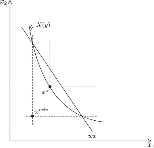
To measure the share of slack that is rationalizable, consider again a firm that has used x to produce y when input prices are w as in Figure 2.

We see that x falls outside the cone dominated by . Hence, not all slack can be rationalized. We see that for x to be produced by an underlying production plan z plus some slack, the underlying production plan will have to be in the (translated) cone . To be able to produce y, it would also have to be above the isoquant of y (i.e., inside ). The least cost of such an underlying production plan is wz in the illustration.
Using this perspective, the total costs of x, wx can be split into three parts.
Unavoidable technical costs. The cost of the allocatively efficient plan xa (i.e., wxa).
Nonrationalizable slack cost. The cost of using z instead of xa as the underlying production plan (i.e., ).
Rationalizable slack cost. The cost of the useful slack x – z (i.e., wx – wz).
The costs of the allocatively efficient plan, wxa, are unavoidable by technological constraints. Additionally, the costs of slack x – z are potentially useful. Thus, we can say that the sum of the two is the rationalizable cost. In contrast, the difference between wxa and wz is nonrationalizable. It represents extra cost that serves no purpose. The firm could have produced the same output and enjoyed the same slack while spending less. We can, therefore, measure the share of rationalizable costsSoRC as
It represents the costs that can be rationalized compared with the total realized costs. SoRC is the share of costs that we can rationalize by the resources being necessary to produce y and by the consumption of useful nonnegative slack.
To formalize these ideas, let us introduce as the minimal cost of a feasible underlying production plan z that dominates the observed input x: that is, as
We see that is the minimal cost of producing y under factor prices w when the underlying production plan z dominates the actual input usage x, , such that we can interpret the extra cost of choosing x instead of z as slack consumption. In Figure 2, we have . Note that by choosing z in Figure 2 as the least costly production plan dominating x, we place the firm in its best possible light by minimizing the cost of the nonrationalizable slack.
Formally, we now have
Note that the share of rationalizable cost SoRC is a value between zero and one because . This follows from the fact that the program is a minimization problem that is restricted compared with the C program. When the SoRC is close to one, this means that the firm’s underlying production plan might have been close to the allocatively efficient point such that there is cost that cannot be rationalized as potentially useful slack.
Of course, there are several related measures of the usefulness of slack that we could have used. One possibility—which is more directly focused on slack—is to compare the cost of useful slack with the cost of slack in total. In our framework, this would be
We do not use this measure for two reasons. First, it does not capture whether slack is only a small part of total resource consumption. In reality, however, total resource consumption is important. Imagine two firms that have both used a total of 1 mio on useful slack and 1 mio on wasteful slack. The two firms would then obtain the same SoRS measure of . This does not capture, however, the relative importance of avoidable spending. If the allocatively efficient costs are 1 mio and 1 billion in the two firms, respectively, the slack consumption is large in the first case and small in the second case. The two firms would, however, obtain the same SoRS measure, namely . In contrast, the SoRC would be very different, namely in the first case and in the second case. This seems to be a more interesting comparison. The first case involves considerable waste, whereas the latter only involves very little waste relative to total spending. In the first case, the firm likely has not optimized at all. In the second case, the slack may be the result of small optimization errors.
Second, using SoRS leads to numerical problems in calculations when some firms are close to operating with an allocatively efficient input vector. In this case, both the numerator and denominator of SoRS are close to zero. When using the SoRC measure instead, the denominator is never close to zero unless outputs y are almost nil.
Let us close the introduction of the SoRC measure by making a few observations about its properties. The SoRC takes values between zero and one. It is one precisely when inputs are dominated by an allocatively efficient input combination. The SoRC is at least as large as cost efficiency and equals cost efficiency, , precisely when a technically efficient mix is chosen; it is at least as large as allocative efficiency , where is Farrell input efficiency (i.e., the largest proportional reduction in all inputs). In a Leontief technology, the SoRC is always one.
The share of rationalizable costs SoRC has the following properties:
SoRC takes values between zero and one,
SoRC = 1 if and only if ,
,
if and only if ,
, and
SoRC = 1 if X(y) is Leontief (i.e., if there exists an such that ).
We have the following.
We have because .
We have
if and only if . In turn, this is equivalent to . Hence, a firm has an SoRC score of one if and only if it is using inputs in the cone above an allocatively efficient plan as in Lemma 2. A similar result is available in corollary 1 in Bogetoft and Hougaard (2003).We have
The last fraction is cost efficiency CE. The first fraction is weakly positive because x is a possible but not necessarily optimal solution to the program. Therefore, we obtain
From this, we have if and only if . The latter is also equivalent to . Hence, SoRC equals cost efficiency if and only if the firm is technically efficient.
Note first that
because Ex is one possibly suboptimal solution to the program. We, therefore, have thatNow using this, we obtain
We, therefore, obtain
where the last inequality follows from and because x is a possible subsolution to the program.When the technology is Leontief, , we have and . Therefore, the estimated slack is nonnegative, , and all costs can be rationalized (i.e., and there is a utility function U(c, s) making x the optimal input combination). □
A property of the SoRC measure, which may prima facie appear counterintuitive and which is shared by the commonly used notion of allocative efficiency, is that a DMU with irrational wasteful slack can increase its SoRC score by using more inputs to produce the same outputs. This property is of course also shared with the original dichotomous notions of rational efficiency
Despite its initial appearance, this property is not entirely counterintuitive. Indeed, cases exist where adding extra slack can make already existing slack more useful. One such case could be a hospital having an excess of doctors. If there is no excess of nurses, the excess doctors may simply be idle without the possibility to scale up production. Thus, increasing the slack in nurses could be beneficial, as a “balanced” slack in both doctors and nurses could insulate the hospital against variations in demand.
Still, in most cases, it is probably not desirable to simply add extra slack. It is, therefore, important to recall that the aim in most organizations is not just to maximize SoRC. Rather, the aim is twofold: to minimize total costs and to pick slack in a rational way.
The logic of the SoRC measure is that DMUs may have preferences for slack and that we do respect these—as long as the other objective, cost minimization, does not suffer more. We do, therefore, require that this slack is acquired in the cheapest possible way. When the same slack is available at a lower total cost, there is a clear Pareto improvement to be gained, and SoRC is less than one.
One of the highest-stakes applications of productivity analysis methods is in the regulation of natural monopolies, like electricity, gas, and water networks (cf., e.g., Bogetoft 1994a, b, 1995, 1997, 2000; Agrell et al. 2005; Agrell and Bogetoft 2017). Here, the goal is typically to minimize spending. However, at the same time, there is a concern—and multiple stories to support it—that maintenance may suffer and that the networks may not be properly prepared for future risks. Further, as maintenance and risk protection are difficult to measure, it is feared that the introduction of an allowance for such activities could be a way to hide suboptimal behavior. In such cases, the dual aim of minimizing costs and maximizing SoRC may be useful. One possibility would be to take a weighted average of cost efficiency and SoRC and use this to determine the allowed revenue, the revenue cap. We leave the examination of regulatory incentive schemes along these lines to future research.
4. Testing
According to the theories of valuable organizational slack, firms care not only about minimizing costs and maximizing profits but also, about the benefits of slack. Therefore, they should ideally make sure to obtain the most possible slack for given cost levels. Our analysis in Section 3.2 showed that this happens when actual inputs are dominated by an allocatively efficient input mix (i.e., when ). Checking this condition, we can classify firms as rational (in our extended sense) or irrational. This is, however, a somewhat blunt approach. In reality, small mistakes may occur in both the estimation of technologies and the choice and implementation of specific strategies. This is why we nuanced the analytical framework with the notion of the share of rationalizable costs, SoRC. A high value of suggests that a large share of all costs can be rationalized in this way. SoRC = 1 means that all costs can be fully rationalized as the result of minimizing costs and maximizing slack, .
In this section, we will discuss different ways to calculate the SoRC measure and test hypotheses about it in empirical applications. In Section 5, we will then provide specific results using two different data sets.
4.1. Calculating the SoRC
We have assumed thus far that we have information about the inputs x used, the outputs y produced, and the input prices w faced by a given firm. In addition, we have assumed that the input requirement set X(y) is known.
In applications, it is often necessary to first estimate the input requirement set. There are a series of possible approaches that can be used, both parametric and nonparametric (cf., e.g., Bogetoft and Otto 2011 for an overview of frontier-based approaches). It is not important which approach is used, but it may of course affect the complications of the following calculations if the technological estimate comes in the form of, for example, a simple (log) linear model, a more complex translog model, or a nonparametric activity-based mathematical programming form. In our numerical applications, we illustrate the latter.
To calculate the SoRC index for a given firm, we need three values, namely the actual costs wx the firm has spent, the minimal costs of producing y when prices are w, and the minimal cost of producing the output y with an input bundle that uses weakly less of all the inputs than the present production plan (). Hence, we typically have to solve two optimization problems:
When we use activity-based analysis to estimate the input requirement set X(y), these optimization problems are typically simple linear or mixed integer linear programming problems. In parametric applications, they are typically simple convex optimization problems with linear objective functions.
4.2. Hypothesis Test: Are Slacks Chosen Randomly?
A large value of SoRC suggests that most of the cost can be rationalized by assuming that firms value slack. However, it is also possible that a large value of SoRC might occur randomly rather than by rational decision making. The probability of randomly selecting an input mix with a high SoRC depends in part on the curvature of the technology. If, for example, the technology is Leontief, all production plans that can produce a given output y can be fully rationalized, SoRC = 1 (cf. Lemma 3). In empirical applications, we would, therefore, prefer to obtain an idea of how difficult it is to rationally choose slack.
We first consider hypothesis tests for an individual firm (firm level) and then, consider hypothesis tests for a group of firms (group level). To simplify the exposition, we have focused on one firm. We will now allow for multiple firms, denoted . We assume that firm k used inputs to produce output and that the input prices faced by firm k are wk. Note that we do not assume that the different firms face the same factor prices. The cost-minimizing input mix can be different for each firm because it also depends on its input prices, its output level, and the prevailing rates of technical substitution between inputs at the selected output level.
4.2.1. Firm Level.
At the individual firm level, we test the following hypothesis for a firm k:
From Lemma 3, we know that a rationally inefficient firm k chooses when it produces yk and faces factor prices wk. We define the binary indicator:
Under H0, , where is the binomial distribution for a single trial with probability of success pk equal to the probability of randomly choosing an input vector in . Let be the specific value of Tk observed. We reject H0 if, under H0,
The indicator Tk is rather blunt, as it does not distinguish between fully irrational (i.e., SoRCk = 0) and somewhat rational inefficient behavior (e.g., ); in both cases, Tk = 0. Only when SoRCk = 1 do we have Tk = 1. Therefore, we can use SoRCk for firm k to construct a more nuanced test statistic. Large values of SoRCk would indicate that firm k tends to select rationalizable slack. In the following, we let SoRCk denote the random variable under H0 and the specific observation hereof.
We might, therefore, reject H0 in favor of HA if the probability under H0 of obtaining a larger value than is at most α (typically 5%): that is, if
The interpretation of a firm k with and for which H0 is rejected is that of costs can be rationalized and that this is significantly higher than expected when assuming that slacks are selected randomly.
These tests may not be very powerful in some cases. When the technology is almost Leontief, for example, separating rational slack from random slack is particularly difficult. In such cases, the random chance of a high SoRCk score or a Tk = 1 value is very high. Hence, we are likely to obtain high values of SoRCk or T = 1 even if the firm selects inputs at random. It is, therefore, very difficult to reject H0.
4.2.2. Group Level.
At the group level, it is easier to perform tests. If we have independent observations of inputs xk, outputs yk, prices wk, and technologies for each of firms, we can test whether firms tend to choose slack rationally: that is,
Similar to the test statistics at the individual level, we can use group indicators such as
The blunt indicator is the number of successes in a sequence of K-independent Bernoulli trials with success probabilities . This resulting distribution is, therefore, a Poisson binomial distribution. We have
When the individual probabilities are given, the probabilities of TK can be calculated recursively as
Alternatively, because we are interested in cases where TK is large, we can for use the Chernoff upper bound (cf. Chernoff 1952):
An open question is of course how sharp this upper bound is.
Exactly how to calculate the distributions of SoRCk and SoRCK and in the case of the blunt statistics, Tk and TK, the values of , again depends on how the technology is described (i.e., how X(y) is defined). With simple parametric specifications, it may be possible to analytically derive the distributions under H0. With more complicated technologies and in particular, with nonparametric, mathematical programming-based estimates of the technology, it is more convenient to bootstrap the distributions. We will now illustrate how to do so.
4.3. Bootstrapping Procedures
To find the distribution of Tk and SoRCk under the null hypothesis, we can randomly draw such that and . Let us assume that we make draws. From this, we obtain observations of and , respectively, and we can use the resulting empirical distribution to compute the p-values as
To implement the bootstrap procedure, we first sample uniformly from a standard p simplex (i.e., , such that and ). This can easily be done by , where (cf. Rubinstein 1982, algorithm 2). Based on λ, we can then construct a corresponding draw of such that . Specifically, we suggest constructing bootstrap samples by
The only potential challenge is that may not be in . If this happens, we simply reject the sampled λ and generate a new one. We repeat this until eventually a sample candidate is accepted and record this as our .
Although the simple rejection sampling procedure works, it is normally too inefficient because many generated samples will be rejected. However, a minor modification can make the sampling procedure much more efficient. Figure 3 illustrates the idea.
When sampling for firm k, we can restrict the sampling space to , where
Any sample that is not dominated by can be rejected because it does not lie in the technology and fulfill the budget constraint. Switching to a new coordinate system with as the origin, sampling within this new coordinate system, and then switching back to the original coordinate system yield
Let us suggest one final possible adjustment of the bootstrapping procedure. When xk is close to being cost efficient, it will usually be difficult to find inputs with the same cost level as xk that are also fully rationalizable. That is, the chance of drawing a random sample for which is very low. Additionally, if xk is a fully cost-efficient input combination, the bootstrap samples all belong to . In such cases, we can, therefore, simply set for all . In the spirit of the Afriat efficiency index in Varian (1990), we can also allow for some “optimization error” by treating any firm k with high cost efficiency, , as cost efficient and setting in the bootstrap.
We also considered alternative bootstrapping approaches. When the technology is estimated using linear programming, we must sample from the intersection of a hyperplane and a convex polytope. To this end, one can resort to a “hit-and-run” procedure using the “hitandrun” package in R (Tervonen et al. 2013, van Valkenhoef et al. 2014). This procedure applies Markov chain Monte Carlo to sample uniformly from convex shapes defined by linear constraints. Unfortunately, the “hit-and-run” procedure proved very slow in our examples, and rejection sampling proved faster in most cases (when ).
4.4. Predictive Success
As discussed, it may be easy to obtain behavior consistent with fully rationalizable slack in some settings. This happens when the set of rationalizable choices (i.e., the intersection of the T = 1 cone and the budget constraint,
In this case, it is not a strong sign of rationalizable cost that T = 1. Bronars (1987) investigated a similar issue about the power of tests of the generalized axioms of revealed preferences. Likewise, studying so-called area theories (i.e., theories that predict a subset of all possible outcomes), Selten (1991) proposed measuring the accuracy of a theory by its relative frequency of correct predictions. A high accuracy may, however, reflect that the predictions are very broad. It is, therefore, relevant to correct for the precision of the theory. The smaller the set of predicted outcomes is relative to the set of all outcomes, the more precise is the hypothesis. A combined measure of predictive success (PS) is now
The PS is the additional accuracy in the predictions of firms’ input choices that is the result of assuming rational choices and not just random choices. If, for example, 80% of all observed outcomes are in a T = 1 cone but 60% will be so in a random draw, the predictive success is only 20%.
In the empirical estimations, we will estimate the predictive success and its components both at the individual level as
In the next section, we will use our framework to analyze two different empirical settings.
5. Empirical Applications
In this section, we illustrate the measures and tests on data from Danish manufacturing companies. In the online appendix, we provide a similar illustration on data from Canadian bank branches.
To model the technology, we will adopt a nonparametric approach and construct an activity analysis model where each firm observation represents one possible activity. Specifically, we use so-called data envelopment analysis (DEA) as described in many textbooks, including Bogetoft and Otto (2011). Based on the K observed production plans , we will estimate the technology
From this, we can directly construct the input requirement set . Using simple linear programming, we can now calculate the different measures of technical efficiency, cost efficiency, allocative efficiency, and SoRC for the different firms.
Before turning to the data, let us note a couple of caveats regarding the use of the SoRC measure in DEA models. It is easy to construct examples where a DMU is rationally inefficient compared with the true frontier but has irrational slack compared with the estimated frontier and vice versa. This is not a problem per se; what you can estimate from a limited sample of observations is almost always different from what you would measure should the underlying truth be known. Still, it is worthwhile emphasizing this fact in connection with DEA models. In DEA, we know that the estimated production possibility set is a subset of the true underlying technology when there is no noise in the data and the underlying true technology fulfills the DEA assumptions about convexity, free disposability, and returns to scale. Hence, we often think of the DEA technology as a cautious, inner approximation of the true technology. This means that estimated Farrell input and cost efficiencies are biased upward. The same is, however, not the case with the usual measure of allocative efficiency, and because SoRC is connected to deviations from allocative efficiency, the SoRC estimate may also be biased both upward and downward. On a related note, one avenue of further developing the theory of rational inefficiency could be to use the hypothesis of rational inefficiency to extend the technology. One could, for example, ask what is the smallest estimated technology that satisfies the general DEA assumptions and makes all (or a certain share of the) observations rationally efficient.
Using data from the public financial accounts of 597 Danish manufacturing companies, we model the production process as a transformation of two inputs, labor cost and depreciation, into one output, gross profit (value added). To cope with yearly fluctuations, we use mean values from 2010 to 2015.
Summary statistics are provided in Table 1. Because both inputs are costs, the input prices in the following will be .
|

Table 1. Descriptive Statistics of Danish Manufacturing Firms
| Mean | Min | Max | Standard deviation | |
|---|---|---|---|---|
| Inputs | ||||
| Labor cost kDKK | 26,507 | 933 | 975,833 | 70,083 |
| Depreciations kDKK | 6,333 | 14 | 433,096 | 28,847 |
| Outputs | ||||
| Gross profit kDKK | 36,432 | 449 | 4,076,500 | 178,412 |
Note. kDKK, 1,000 Danish Crowns.
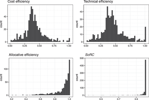
Figure 4 shows histograms for the cost, technical, and allocative efficiencies as well as SoRC. We see that only 20 firms are technically efficient (i.e., are producing on the technological frontier). This occurs because of the relatively small model with only two inputs and one output. Six of these are also produced with cost-minimizing inputs and are, therefore, cost efficient. The interesting question is now how many of the firms can claim to have spent extra costs in a rational manner. We see that this is actually the case for a large share of the firms; 472 firms have an SoRC value of one, and 507/597 (85%) of the firms have an SoRC above 99%.
To test H0 that firms randomly select inputs, we can use the blunt statistic , showing that 472 of the 597 firms are located inside the cone with T = 1. The corresponding p-value is 0.20 using the bootstrapping procedure (B = 2,000 with ). Hence, despite the many observations with T = 1, we cannot reject the H0 hypothesis of randomly chosen inputs. The probability density obtained from the bootstrap is shown in Figure 5(a). For comparison, we also computed the Chernoff bound, which gave a p-value of 0.94. (The probability of success pk for trial k is calculated from , with being the indicator function. The mean of the Poisson binomial distribution, , lies close to the test statistic ().) Thus, the Chernoff bound does not provide a close bound in this case.

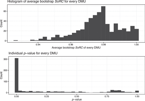
Instead of the somewhat blunt TK measure, we can, as suggested, consider the mean of the SoRC values , with large values leading to rejection of H0. Comparing this once again with the bootstrapped distribution depicted in Figure 5(b), we can now see that under H0, it is difficult to obtain higher average SoRCk values than in our current sample. We find a p-value of . Thus, we reject the H0 hypothesis of random slack choice. Data certainly support the idea that firms introduce mainly rational or useful slack.
Regarding the individual firms, we saw already that 472 firms have an SoRC value of one, and 507/597 (85%) of the firms have an SoRC above 99%. Therefore, most individual firms consume almost exclusively useful slack. Regarding statistical significance, we need to account for the structure of the production technology and the likelihood of randomly obtaining high values of SoRC. The bootstrap yields measures for every firm for bootstrap iterations. The upper chart in Figure 6 shows the histogram of mean bootstrapped SoRC values for each of the firms (i.e., of for all firms k). From the samples, we can also calculate the individual p-values using firm-level bootstrap measures . In our sample, we find that 329/597 (55.11%) of the firms have p-values less than or equal to . The lower chart in Figure 6 shows the histogram of these individual p-values. Thus, we can say that for 329 individual firms, we must reject the idea of random slack choice. They choose slack that is significantly more rational than can be expected by random behavior.
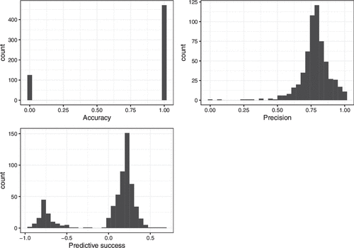
Another way to interpret the large SoRC values and the large share of firms with significantly larger SoRC than what would be expected under H0 is in terms of the power of the tests. The panels in Figure 7 show histograms of the accuracy, precision, and predictive success for individual manufacturing firms. We see that 464 (77.72%) of the firms have a predictive success of more than zero (i.e., for 77.72% of the firms, it helps explain their input choices to assume that they choose inputs rationally).
Finally, let us comment briefly on the effectiveness of the bootstrapping procedure we used. We never needed to resample to cope with problems of an initial sample being rejected. This is in sharp contrast to our next example and is intuitively the result of having a large data set that spans the frontier of a simple model with only two inputs and one output.
6. Final Remarks
From the perspective of organizational theory, slack can be useful (e.g., it can serve as a cushion for a firm when it is hit by an external shock). Economists typically view slack as wasteful; slack is caused by inefficiencies that are harmful to the firm’s profitability and its position in the market. Therefore, slack needs to be eliminated.
This paper offers an approach to reconcile both strands of literature. We acknowledge that slack may be both useful and wasteful. The challenge is how to separate the two and to do so in a relatively general setting. Our approach relies on the simple Pareto principle. If an organization can maintain the same levels of output and slack at a lower cost, there is wasteful or nonrationalizable spending. Using this idea, we proposed measuring the share of rationalizable costs SoRC as the rationalizable costs compared with the total costs.
We also showed how to test whether observed SoRC values are sufficiently large to conclude that individual firms or sectors are choosing slack rationally. The challenge in these tests is to determine how the properties of the technology affect the chances of choosing inputs at random that resemble rationalizable inputs. Bootstrapping can be used to estimate the effects of random slack selection in a specific technology.
We have applied our methodology to two data sets. For Danish manufacturing firms, we found that the outcomes gave strong support to the rational choice hypothesis. In the online appendix, we report on an application to Canadian bank branches. Here, the conclusions were pessimistic. Random choice of inputs would in general look more rationalizable than the actual observations. In both cases, we estimated the production structures from the data using nonparametric best-practice technologies.
There are many possible extensions of the analyses in this paper. Let us mention just a few.
In our approach, we seek to explain as much of the observed practices as the result of rational behavior. This also means that we attempt to minimize the extra cost of irrational behavior. We think this is a natural approach in line with the basic idea of placing the evaluated in their best possible light. On the other hand, one could also take the other approach of maximizing the costs associated with irrationality. This is technically simple. We could just maximize instead of minimize in the definition of . Taking both approaches, one would obtain an interval of possible SoRC values and perhaps a way to discriminate better between firms whose behavior cannot be fully rationalized.
It would be relevant to tighten the nonparametric tests by also considering parametric tests. Instead of assuming H0 that random inputs are chosen uniformly on the isocost curves, one might assume that some input combinations are more likely than others. In firms and organizations, some input factors are likely more powerful negotiators than others and are, therefore, likely to extract more slack than others; see also the discussion in Bogetoft and Hougaard (2003). An alternative reason to deviate from uniform input selections on the isocost curve may be to limit information rents. Recent research shows that with limited information about the cost structure, principals may favor input and output mixes that are closer to historical mixes (cf. Antle and Bogetoft 2019).
It would also be relevant to make additional empirical applications where the derived SoRC measure is linked with other performance measures (e.g., accounting-based measures, as discussed in Section 2) or with indications of the management practices used. Recent research has shown that greater implementation of structured management practices (e.g., careful monitoring, clear targeting practices, and strong incentives) is associated with higher productivity, profitability, and survival rates; see, for example, Bloom and Van Reenen (2007) and Bloom et al. (2014). It would be interesting to link such a systematic description of practices with the SoRC measure.
The authors thank two anonymous reviewers and the editors for their constructive comments that have improved the paper. The usual disclaimer applies.
References
- (1972) Efficiency estimation of production functions. Internat. Econom. Rev. 13(4):568–598.Crossref, Google Scholar
- (2017)
Theory, techniques and applications of regulatory benchmarking and productivity analysis . Grifell-Tatjé E, Knox Lovell CA, Sickles RC, eds. The Oxford Handbook of Productivity Analysis (Oxford University Press, Oxford, United Kingdom), 523–555.Google Scholar - (2005) DEA and dynamic yardstick competition in scandinavian electricity distribution. J. Productivity Anal. 23(2):173–201.Crossref, Google Scholar
- (2019) Mix stickiness under asymmetric cost information. Management Sci. 65(6):2787–2812.Link, Google Scholar
- (2009) Rationalising DEA estimated inefficiencies. J. Bus. Econom. 4:81–86.Google Scholar
- (2013a) Rationalizing inefficiency: Staff utilization in branches of a large Canadian bank. Omega 41(1):80–87.Crossref, Google Scholar
- (2013b) Testing over-representation of observations in subsets of a DEA technology. Eur. J. Oper. Res. 230(1):88–96.Crossref, Google Scholar
- (1988) Nonparametric analysis of technical and allocative efficiencies in production. Econometrica 56(6):1315–1332.Crossref, Google Scholar
- (1996) The quickhull algorithm for convex hull. ACM Trans. Math. Software 22(4):469–483.Crossref, Google Scholar
- (1938) Functions of the Executive (Harvard University Press, Cambridge, MA).Google Scholar
- (2007) Measuring and explaining management practices across firms and countries. Quart. J. Econom. 122(4):1351–1408.Crossref, Google Scholar
- (2014) The new empirical economics of management. J. Eur. Econom. Assoc. 12(4):835–876.Crossref, Google Scholar
- (1994a) Incentive efficient production frontiers: An agency perspective on DEA. Management Sci. 40(8):959–968.Link, Google Scholar
- (1994b) Non-Cooperative Planning Theory (Springer-Verlag, Berlin).Crossref, Google Scholar
- (1995) Incentives and productivity measurements. Internat. J. Production Econom. 39(1):67–81.Crossref, Google Scholar
- (1997) DEA-based yardstick competition: The optimality of best practice regulation. Ann. Oper. Res. 73:277–298.Crossref, Google Scholar
- (2000) DEA and activity planning under asymmetric information. J. Productivity Anal. 13:7–48.Crossref, Google Scholar
- (2009) Rational inefficiency in fishery. J. Bus. Econom. 4:63–79.Google Scholar
- (2003) Rational inefficiencies. J. Productivity Anal. 20:243–271.Crossref, Google Scholar
- (2011) Benchmarking with DEA, SFA, and R (Springer, New York).Crossref, Google Scholar
- (1981) On the measurement of organizational slack. Acad. Management Rev. 6(1):29–39.Crossref, Google Scholar
- (2011) Swinging a double-edged sword: The effect of slack on entrepreneurial management and growth. J. Bus. Venturing 26:537–554.Crossref, Google Scholar
- (1991) Testing a causal model of corporate risk taking and performance. Acad. Management J. 34(1):37–49.Crossref, Google Scholar
- (1987) The power of nonparametric tests of preference maximization. Econometrica 55(3):693–698.Crossref, Google Scholar
- (1990) A nonparametric analysis of productivity: The case of U.S. and Japanese manufacturing. Amer. Econom. Rev. 80(3):450–464.Google Scholar
- (1993) On generalized revealed preference analysis. Quart. J. Econom. 108(2):493–506.Crossref, Google Scholar
- (1995) On non-parametric supply response analysis. Amer. J. Agricultural Econom. 77(1):80–92.Crossref, Google Scholar
- (1997) Statistical applications of the Poisson-binomial and conditional Bernoulli distributions. Statist. Sinica 7:875–892.Google Scholar
- (1952) A measure of asymptotic efficiency for tests of a hypothesis based on the sum of observations. Ann. Math. Statist. 23(4):493–507.Crossref, Google Scholar
- (1963) A Behavioral Theory of the Firm (Prentice-Hall, Englewood Cliffs, NJ).Google Scholar
- (2004) Slack resources and firm performance: A meta-analysis. J. Bus. Res. 57(6):565–574.Crossref, Google Scholar
- (1951) The coefficient of resource utilization. Econometrica 19(3):273–292.Crossref, Google Scholar
- (1995) Non-parametric tests of regularity, Farrell efficiency, and goodness of fit. J. Econometrics 69(2):415–425.Crossref, Google Scholar
- (1957) The measurement of productive efficiency. J. Royal Statist. Soc. Series A 120(3):253–281.Crossref, Google Scholar
- (1973) Designing Complex Organizations (Addison-Wesley, Reading, MA).Google Scholar
- (1974) Organizational design: An information processing view. Interfaces 4(3):28–36.Link, Google Scholar
- (1972) Testing assumptions of production theory: A nonparametric approach. J. Political Econom. 80(2):256–275.Crossref, Google Scholar
- (2006) What is the relationship between organizational slack and innovation? J. Management Issues 18(3):372–392.Google Scholar
- (2010) Lean and hungry or fat and content? Entrepreneurs’ wealth and start-up performance. Management Sci. 56(8):1242–1258.Link, Google Scholar
- (1976) Theory of the firm: Managerial behavior agency cost and ownership structure. J. Financial Econom. 3(4):305–360.Crossref, Google Scholar
- (1951) Activity Analysis of Production and Allocation (Wiley, New York).Google Scholar
- (1966) Allocative efficiency vs. ‘X-efficiency.’ Amer. Econom. Rev. 56(3):392–415.Google Scholar
- (1978) X-inefficiency Xists: Reply to an Xorcist. Amer. Econom. Rev. 68:203–211.Google Scholar
- (1958) Organizations (Wiley, New York).Google Scholar
- (2010) In defense of bureaucracy: Public managerial capacity, slack and the dampening of environmental shocks. Public Management Rev. 12(3):341–361.Crossref, Google Scholar
- (2013) The too-much-of-a-good-thing effect in management. J. Management 39(2):313–338.Crossref, Google Scholar
- (1982) Generating random vectors uniformly distributed inside and on the surface of different regions. Eur. J. Oper. Res. 10(2):205–209.Crossref, Google Scholar
- (1947) Foundations of Economic Analysis (Harvard University Press, Cambridge, MA).Google Scholar
- (1991) Properties of a measure of predictive success. Math. Social Sci. 21(2):153–167.Crossref, Google Scholar
- (1994) On the distribution of the sum of independent integer valued random variables. Amer. Statist. 27(3):123–124.Google Scholar
- (1970) Theory of Cost and Production Functions (Princeton University Press, Princeton, NJ).Google Scholar
- (1986) Performance slack and risk taking in organizational decision making. Acad. Management J. 29(3):562–585.Crossref, Google Scholar
- (1976) The xistence of x-efficiency. Amer. Econom. Rev. 66(1):213–216.Google Scholar
- (2003) Organizational slack and firm performance during economic transitions: Two studies from an emerging economy. Strategic Management J. 24(13):1249–1263.Crossref, Google Scholar
- (2013) Hit-and-run enables efficient weight generation for simulation-based multiple criteria decision analysis. Eur. J. Oper. Res. 224(3):552–559.Crossref, Google Scholar
- (2007) Effect of firm resources on growth of multinationality. J. Internat. Bus. Stud. 38(6):961–974.Crossref, Google Scholar
- (2014) Notes on ‘hit-and-run enables efficient weight generation for simulation-based multiple criteria decision analysis.’ Eur. J. Oper. Res. 239(3):865–867.Crossref, Google Scholar
- (1984) The non-parametric approach to production analysis. Econometrica 52(3):279–297.Crossref, Google Scholar
- (1985) Non-parametric analysis of optimizing behavior with measurement error. J. Econometrics 30(1):445–458.Crossref, Google Scholar
- (1990) Goodness-of-fit in optimizing models. J. Econometrics 46:125–140.Crossref, Google Scholar
- (1963) Managerial descretion and business behavior. Amer. Econom. Rev. 53(5):1032–1057.Google Scholar
Peter Bogetoft is a full professor in applied microeconomics at Copenhagen Business School. He has published seven books and around 100 scientific articles. He has also been involved in a series of consultancy projects on the application of theories, in particular with respect to contract design, transfer pricing, auction design, regulation, and benchmarking, and he is a founding father of several research spin-offs.
Pieter Jan Kerstens is a researcher at the Flemish Institute for Technological Research and a voluntary researcher in the Department of Economics at Katholieke Universiteit Leuven. His main research interest is production economics with a focus on nonparametric efficiency analysis and productivity.

