


Generating Lagrangian Cuts Using Normalized Dual Problems in Multistage Stochastic Mixed-Integer Programming
Abstract
Based on recent advances in Benders decomposition and two-stage stochastic integer programming, we present a framework to generate Lagrangian cuts in multistage stochastic mixed-integer linear programming by solving normalized dual problems. This framework can be incorporated into existing solution methods, such as stochastic dual dynamic integer programming. We show how different normalizations can be applied in order to generate cuts satisfying specific properties with respect to the convex hull of the epigraph of the value functions (e.g., having a maximum depth or being facet defining). We provide computational results to evaluate the efficacy and performance of this approach, showing that compared with existing techniques from the literature, significantly better lower bounds can be obtained.
History: Accepted by Andrea Lodi, Area Editor for Design & Analysis of Algorithms–Discrete.
Funding: The research of C. Füllner was funded by the Deutsche Forschungsgemeinschaft [Grant 445857709]. A research visit of C. Füllner at the Georgia Institute of Technology was funded by the Karlsruhe House of Young Scientists. The research of X. A. Sun was partially funded by the National Science Foundation [CAREER Award 2316675].
Supplemental Material: The software that supports the findings of this study is available within the paper and its Supplemental Information (https://pubsonline.informs.org/doi/suppl/10.1287/ijoc.2024.1039) as well as from the IJOC GitHub software repository (https://github.com/INFORMSJoC/2024.1039). The complete IJOC Software and Data Repository is available at https://informsjoc.github.io/.
1. Introduction
In this paper, we study the generation of Lagrangian cuts in decomposition methods for solving multistage stochastic mixed-integer linear programs (MS-MILPs), such as stochastic dual dynamic integer programming (SDDiP) (Zou et al. 2019). We present a framework to generate Lagrangian cuts with favorable properties by solving special normalized Lagrangian dual problems.
1.1. Motivation and Prior Work
Multistage stochastic programs are relevant to model decision-making processes in practice because often, sequential decisions have to be made over a finite number of stages and under uncertainty considering the problem data of the following stages. For the solution of these problems, tailored decomposition methods are most widely used; stochastic dual dynamic programming (SDDP) is among the most prominent ones (Pereira and Pinto 1991). These methods decompose the large-scale problem into stage- and scenario-specific subproblems coupled by state variables and so-called value functions, which are denoted . For linear problems, these functions are convex polyhedral and can be exactly represented by finitely many affine functions called cuts (Benders 1962). However, in many applications, some of the decision variables have to be integer or binary. In this case, we obtain an MS-MILP, and the value functions are in general nonconvex and discontinuous.
A key challenge is that in this case, linear cuts, such as Benders cuts, are in general not sufficient to ensure (almost sure) finite convergence of SDDP-like decomposition methods as they are no tight approximators of . Recently, more focus has been put on Lagrangian cuts, which are constructed by solving special Lagrangian dual problems and stronger than Benders cuts (Zou et al. 2019) as they can recover the closed convex envelope of (Füllner et al. 2024). Even more, in the special case that all state variables are binary, Lagrangian cuts are tight for . This is at the core of the SDDiP algorithm. Using a binary approximation of the state space, SDDiP can also be applied to general MS-MILPs with convergence guarantees (Zou et al. 2019).
Nonetheless, applying Lagrangian cuts in practice comes with some considerable challenges.
Even if the Lagrangian dual is a convex optimization problem, it may be very costly to solve repeatedly because of its nonsmooth objective function. This is only aggravated if the state space is artificially increased by a binary approximation for general MS-MILPs.
Lagrangian dual problems are often degenerate with multiple optimal solutions, and the cuts associated with some of these solutions can be very weak. This issue is especially common for the binary state space required in SDDiP because all cuts are constructed at extreme points. It is, therefore, important not only to solve the dual problem but also, to identify a solution that yields a strong cut.
Whereas tight cuts are sufficient to ensure theoretical convergence of SDDiP, (solely) relying on them in practice may lead to very slow convergence. At worst, a complete enumeration of the binary state space is required. It is plausible that there exist alternative (even nontight) cuts that may significantly speed up the convergence process.
Some first attempts to address these challenges have been made recently, mostly with respect to (a) and (c). In the original SDDiP paper, it was proposed to combine tight cuts with strengthened Benders cuts that are not tight in general but stronger than Benders cuts and efficient to compute (Zou et al. 2019). Similarly, a scheme alternating between Lagrangian and Benders cuts is proposed by Bansal and Küçükyavuz (2026). Rahmaniani et al. (2020) present a heuristic to generate Lagrangian cuts more efficiently using inner approximations or partial relaxations. For two-stage stochastic problems, Chen and Luedtke (2022) suggest to restrict the dual feasible set to the span of Benders cut coefficients of previous iterations, thereby losing tightness guarantees but obtaining reasonably good Lagrangian cuts in short time. With respect to (b), Deng and Xie (2024) propose to first generate cheap and tight but weak integer optimality cuts and then, to solve some auxiliary linear programs (LPs) to strengthen them in order to obtain strong Lagrangian cuts.
In addition, there has been a lot of research on alternative cut-generation techniques addressing challenge (b), yet for Benders cuts in Benders decomposition (BD) instead of Lagrangian cuts, see Table 1. To address degeneracy and weak cuts, Magnanti and Wong (1981) present a two-step approach to generate Pareto-optimal cuts. Their ideas are improved by Papadakos (2008), who shows that it is sufficient to solve a single optimization problem. Sherali and Lunday (2013) propose to generate certain maximally nondominated Benders cuts by solving a perturbation of the original subproblem. Glomb et al. (2026) introduce so-called optimal line-shifting cuts satisfying a novel notion of Pareto optimality.
|

Table 1. Examination of Cut-Quality Criteria in the Literature on BD and Disjunctive Programming
| Paper | MIS | Maximal depth | Facet defining | Pareto optimality |
|---|---|---|---|---|
| Magnanti and Wong (1981) | ✓ | |||
| Cornuéjols and Lemaréchal (2006) | ✓ | ✓ | ||
| Papadakos (2008) | ✓ | |||
| Cadoux (2010) | ✓ | ✓ | ||
| Fischetti et al. (2010) | ✓ | |||
| Sherali and Lunday (2013) | ✓ | |||
| Conforti and Wolsey (2019) | ✓ | |||
| Brandenberg and Stursberg (2021) | ✓ | ✓ | ✓ | |
| Seo et al. (2022) | ✓ | |||
| Hosseini and Turner (2025) | ✓ | ✓ | ||
| Glomb et al. (2026) | ✓ | |||
| This paper | ✓ | ✓ | ✓ |
Note. MIS, cuts that correspond to minimal infeasible subsytems of the feasibility subproblem.
A novel epigraph-based perspective on generating Benders cuts is introduced in Fischetti et al. (2010). In contrast to standard BD, by using a formulation with an additional dual multiplier, the proposed cut-generation problem allows us to generate optimality and feasibility cuts in a unified way. On the flip side, the cut-generation problem is unbounded without further adjustments. Therefore, the authors suggest to solve a special normalized version instead.
The formulation from Fischetti et al. (2010) allows for different normalization techniques and by that, the generation of cuts satisfying different quality criteria. Hosseini and Turner (2025) show how normalizations can be used to generate deep cuts in BD, which are characterized by maximizing the distance between the separating hyperplane and the incumbent to separate, a property that is also explored in Cornuéjols and Lemaréchal (2006) and Cadoux (2010). By relating the cut generation to the so-called reverse polar set, Brandenberg and Stursberg (2021) show how facet-defining and Pareto-optimal cuts can be generated in BD using linear normalizations (LNs). The same cut-generation procedure is put forward by Seo et al. (2022) but motivated from a different geometric perspective. An alternative yet related approach to generate facet-defining cuts is presented by Conforti and Wolsey (2019).
Many of these approaches are reported to lead to significant performance improvements compared with standard BD. Therefore, it seems reasonable to explore how they (or similar ideas) can be translated to stochastic programming and Lagrangian cuts. A first attempt in this direction is the work by Chen and Luedtke (2022). They apply the unified cut-generation perspective from Fischetti et al. (2010) and a special normalization to generate Lagrangian cuts in branch-and-cut methods to solve two-stage stochastic mixed-integer linear programs (MILPs).
1.2. Contribution
In this paper, similar to Chen and Luedtke (2022), we apply the unified perspective from Fischetti et al. (2010) to the multistage stochastic case, and based on this, we present a general framework with which Lagrangian cuts of various styles can be generated within decomposition methods for MS-MILPs. We show that as for BD, different normalization techniques in the Lagrangian dual lead to Lagrangian cuts with distinct properties, such as maximal depth, Pareto optimality, or being facet defining with respect to .
Compared with the work by Chen and Luedtke (2022), our work differs in several aspects. First, we consider a formulation for the multistage case, even though the extension from the two-stage case is straightforward. Second, we consider a variety of possible normalization techniques for the Lagrangian dual, including different norms and linear functions. In contrast, Chen and Luedtke (2022) focus on a specific type of normalization using the 1-norm that is directly linked to their idea of restricting the dual feasible set. Third, they solve two-stage stochastic problems using a branch-and-cut method. Stronger cuts can help accelerate the solution process in these methods but are not required to achieve convergence. Therefore, the authors’ main focus is the computationally efficient generation of reasonably strong (yet not necessarily supporting) Lagrangian cuts, thus addressing challenges (a) and (c). We, on the other hand, explore in detail the effect of different normalizations on the theoretical properties of the Lagrangian cuts with the aim of satisfying certain quality criteria. Hence, our work mostly addresses challenge (b) above. As the new Lagrangian cuts do not satisfy the traditional notion of tightness but lead to better lower bounds (LBs) in our computational tests, our work also refers to challenge (c). Even more, we show that using our proposed cut-generation framework, convergence of SDDiP can still be assured.
Compared with the existing literature on BD, our work differs as well. First, we apply the cut-generation formulation from Fischetti et al. (2010) to the stochastic and Lagrangian setting. Second, we apply various normalization concepts from the literature on BD and show how they and the properties of the obtained cuts translate to this setting. A notable difference in the Lagrangian setting is that we do not tightly approximate itself but for which no explicit description is readily available. This also limits the applicability of certain techniques that are tailored to BD. Finally, the MS-MILP setting poses several challenges for the computation of core points that the linear normalizations that we use rely on, among them infeasibility as well as aggravated verification of core-point candidates. For this reason, we propose several heuristics to identify core points in our specific setting. We run extensive computational tests to evaluate their performance.
The key contributions of this paper are summarized again below.
We show how the unified cut-generation formulation for BD from Fischetti et al. (2010) can be applied to the generation of Lagrangian cuts for MS-MILPs. This idea has already been used by Chen and Luedtke (2022) in two-stage stochastic MILPs, but it has not been extended to the multistage case yet.
As the obtained Lagrangian dual problems are unbounded, some normalization is required to select cut coefficients in a reasonable way. We draw on recent concepts for cut selection in BD, such as optimizing over the reverse polar set (Brandenberg and Stursberg 2021) or generating deep cuts (Hosseini and Turner 2025), and we translate them to the stochastic and Lagrangian setting. This way, we obtain a variety of different normalization techniques and by that, generalize the cut-generation approach from Chen and Luedtke (2022). We further show that different normalization techniques in the Lagrangian dual lead to Lagrangian cuts with distinct properties, such as maximal depth, Pareto optimality, or being facet defining with respect to .
We show that linear normalizations are closely related to the identification of core points in the epigraphs , which can be challenging for MS-MILPs. Therefore, we propose four heuristic approaches for the computation of core-point candidates and study them computationally.
Our proposed cut-generation framework can be incorporated into SDDiP and related decomposition methods. We prove that under some assumptions, still (almost sure) finite convergence of these methods can be guaranteed.
We perform extensive computational tests for SDDiP incorporating our cut-generation approach on two known test problems from the literature. We show that the obtained lower bounds in SDDiP are majorly improved compared with conventional cuts. However, we also observe that this does not in all cases lead to an improvement of the obtained policies and that solving the Lagrangian dual problem remains a computational challenge.
For reasons of space, some details, including all technical proofs, are moved to the Online Appendix.
2. Problem Formulation
We start by introducing MS-MILPs and their decomposition formally. We consider a finite number of stages, where some of the problem data are uncertain and evolve according to a known stochastic process with deterministic . We assume that the random data vectors are discrete and finite such that the uncertainty can be modeled by a finite scenario tree. Let denote the set of nodes of this tree. For each node , the unique ancestor node is denoted by , and the set of child nodes is denoted by . The probability for some node n is and assumed to be known. The transition probabilities between adjacent nodes can then be determined as . For the root node r, we assume and . We define to address the set of nodes without the root node and to address the set of nodes without leaf nodes, and we denote by the nodes at stage t.
For each node , we distinguish state variables , which also appear in child nodes of n, and local variables . denotes the objective function of node n, and denotes the feasible set of node n, which depends on the state variable from the ancestor node. We assume that is a linear function in and and that is a mixed-integer polyhedral set for all defined by
Here, denote appropriately defined data matrices and vectors. The sets and are intersections of polyhedral sets and possible integrality constraints. In the following, we also refer to as the state space.
An MS-MILP can then be expressed by its dynamic programming equations. For the root node, we obtain
For the leaf nodes , we set . Moreover, we set if , and we denote by the effective domain of . Furthermore, we denote by its closed convex envelope, the point-wise supremum of all affine functions majorized by .
Note that regarding as a function on is not standard in stochastic programming. Often, it is (implicitly) assumed to be defined only on the domain . However, from our view, allowing to be defined on with extended real values appears more suitable for the following steps.
As this proves beneficial in the cut-generation process, we introduce local variables and accompany them with copy constraints and constraints , with . The most natural choice is , but also, other choices are possible (e.g., ). For more details, we refer to Füllner et al. (2024). This reformulation yields the equivalent subproblems
For the remainder of this article, we make some basic assumptions.
The following conditions are satisfied by (1)–(3).
A1. For all , the sets and are compact.
A2. For all , all coefficients in , , , and are rational.
A3. For all , is compact, rational MILP representable, and .
Note that property (A1) of Assumption 1 immediately implies that is bounded for all and . Property (A3) of Assumption 1 and the way that is defined imply relatively complete recourse, a standard assumption in stochastic programming. We obtain the following standard properties for the value functions.
For all , the value functions are proper, lower semicontinuous, and piecewise polyhedral with finitely many pieces.
By applying the properness reasoning to the root node, we conclude that is finite.
3. Generating Lagrangian Cuts with Normalized Dual Problems
In this section, we present a framework for the generation of Lagrangian cuts when solving MS-MILPs that serves as an alternative to the classical Lagrangian cut-generation framework from SDDiP (Zou et al. 2019) (see Online Appendix EC.1 for comparison). The framework is based on three key ingredients.
It uses the idea of the unified cut-generation formulation for BD from Fischetti et al. (2010) and applies it to MS-MILPs to derive a special Lagrangian dual problem. This is the subject of Sections 3.1 and 3.2. The dual problem generalizes the one used by Chen and Luedtke (2022) to the multistage case.
As this dual problem is unbounded, our framework also follows the aforementioned works in applying a normalization. Deviating from the static normalization (Fischetti et al. 2010) and the -norm normalization (Chen and Luedtke 2022) used in these works, our framework allows for general normalizations. We discuss different options using norms and linear functions, and we explore the impact on the properties of the obtained Lagrangian cuts. This is the subject of Sections 3.3–3.5.
When a linear normalization is used, knowledge of a core point within is required, which can be challenging to achieve for MS-MILPs. We thus present different heuristics for that purpose. This is the subject of Section 3.6.
Algorithm 1 provides a general overview on the cut-generation framework.
(
Require: Subproblem (6) for node with index i. NORM = true or NORM = false.
1: Solve Subproblem (6) to obtain and for all .
2: for child node do
3: ifNORM = true then
4: Choose some norm , and set up the dual problem (11) for m and i with .
5: else
6: Use heuristics Mid, Eps, Relint, or Conv from Section 3.6 to compute a core-point candidate .
7: Compute coefficients .
8: Set up the dual problem (11) for m and i with .
9: Solve the dual problem (11) for m and i, and store the multipliers .
10: Construct a cut of form (10).
11: Use the cut to update the set to in Subproblem (6) for node n.
3.1. An Epigraph Perspective on Cut Generation
We first introduce the cut-generation perspective from Fischetti et al. (2010) yet tailor it to our case of MS-MILPs. Recall the definition of the epigraph of the value functions :
We can use this definition to reformulate Subproblems (3) to
Here and in the following, we use as a shortened notation for .
The condition from the definition in (4) is always satisfied implicitly in Problem (5) because by Assumption 1 and by construction.
In classical BD, iteratively optimality cuts are constructed to approximate , and if required, feasibility cuts are constructed to approximate . This is done by solving distinct cut-generation problems. However, from (4), it is evident that both types of cuts actually approximate . Therefore, we may as well consider a unified cut-generation problem to obtain polyhedral approximations of the sets (Fischetti et al. 2010). Although the need for feasibility cuts is ruled out by property (A3) of Assumption 1 in our setting here, the unified cut-generation framework still proves itself valuable as we shall see.
In multistage stochastic programming, cuts are often aggregated to obtain single cuts for the expected value functions (single-cut approach) as this reduces the total number of cuts in the subproblems. The unified perspective here requires a separate set of approximations for each (multicut approach) instead as it uses distinct values in the cut-generation process.
As the value functions are not known explicitly, for the cut-generation process, we replace each occurrence of in (5) with its current approximation (with iteration index i). This way, we actually generate cuts for . However, by construction, they also yield outer approximations of . To avoid unboundedness, each set is initialized with a valid outer approximation .
For notational simplicity, for the remainder of this paper, we define the set
We make another assumption for the remainder of this paper.
For all and all iterations i, all linear cuts defining the polyhedral set are defined by rational coefficients.
Furthermore, we later require the following result for the convex hull of set .
The set is a closed convex polyhedron. That means that there exist matrices and a vector such that .
3.2. An Unbounded Lagrangian Dual Problem
We now address the cut-generation process in the unified framework. Given a point , we consider the feasibility problem
To generate Lagrangian cuts, we apply a Lagrangian relaxation to Problem (7). A key difference to the classical Lagrangian relaxation from SDDiP (see Online Appendix EC.1) is that not only , but is regarded as a fixed incumbent for the cut-generation process. Therefore, we relax all constraints containing either or . For given multipliers , the dual function is then given by
The Lagrangian dual problem, which corresponds to the one used by Chen and Luedtke (2022) for the two-stage case, is
We state some important properties of this dual problem, with a proof provided in Online Appendix EC.2.2.
The optimal value of the Lagrangian dual (9) satisfies
Theorem 1 implies that the Lagrangian dual is unbounded whenever . Therefore, there exists an unbounded ray such that , and violates the following Lagrangian cut.
For all and some multipliers , a Lagrangian cut is given by
This cut is valid for any feasible in (9) as proven in Online Appendix EC.2.3.
For any , the Lagrangian cut (10) is satisfied by all and thus, by all .
3.3. A Normalized Lagrangian Dual Problem
It is not immediately clear how to select cut coefficients from the unbounded Lagrangian dual (9) in the most reasonable way. Therefore, we consider a normalized problem instead.
For some homogeneous normalization function , the normalized Lagrangian dual is defined as
As long as the normalization constraint is satisfied by some neighborhood N of the origin, we do not exclude any potential cuts because of the scaling property of ; see Remark EC.1 in Online Appendix EC.1 and Chen and Luedtke (2022).
Fischetti et al. (2010) use and an adjustment accounting for zero entries in the problem matrices. Chen and Luedtke (2022) propose with a possible adjustment tailored to their reduction of the dual space.
Problem (11) can be solved using the Kelley cutting-plane method (Kelley 1960) as presented in Online Appendix EC.6 or using related bundle methods (Lemaréchal et al. 1995).
The normalized problem has the following important property.
If , then and vice versa.
We provide a proof in Online Appendix EC.2.4. Lemma 3 allows us to solely focus on the case where for the remainder of this section.
The reasons to consider a normalization of the unbounded Lagrangian dual (9) are twofold. On the one hand, we aspire to determine coefficients by solving a bounded and feasible optimization problem. A common approach to achieve this is to fix its unbounded objective to one. Combined with Remark 4, this allows us to identify unbounded rays by analyzing a compact polyhedron (Fischetti et al. 2010). Alternatively, it can be achieved by bounding Problem (9) artificially (e.g., by introducing bounds on the dual multipliers or by introducing a carefully designed normalizing constraint).
On the other hand, in the light of challenge (b) presented in Section 1.1, we want to make sure that the obtained cuts do not only separate the incumbent from but also, are of good approximation quality. As stated in Table 1 in Section 1.1, various quality criteria for cutting planes have been put forward in the literature. We focus on three important criteria here.
Maximizing cut depth. Deep cuts realize a maximum distance between the incumbent and the separating hyperplane (i.e., they cut as deeply as possible into the suboptimal region).
Being facet defining. Facet-defining cuts reproduce (some of the finitely many) facets of a convex polyhedral set: in our case, .
Pareto optimality (Magnanti and Wong 1981). For , Pareto-optimal cuts (10) are nondominated in the sense that there exists no other cut such that
for all . Importantly, Pareto optimality with respect to does not necessarily imply Pareto optimality with respect to but is easier to achieve.
As shown in the literature on BD, many of these criteria can be satisfied by optimizing over the so-called reverse polar set of shifted by the incumbent , which provides a characterization of normal vectors of -separating hyperplanes and thus, is an important tool in the theory on cut generation (Cornuéjols and Lemaréchal 2006, Brandenberg and Stursberg 2021).
The reverse polar set was first introduced by Balas and Ivanescu (1964) and can be defined as follows.
The reverse polar set of a set is defined as .
To simplify notation, we set for the reverse polar set of shifted by . Using Remark 4, it can be reformulated.
The reverse polar set can be expressed as
We provide a proof in Online Appendix EC.2.5.
Even with the above reformulation of , an explicit formulation is usually not readily available because of the existence quantor and because of , and not being known.
Even though is not known explicitly, it proves useful in the derivation of Lagrangian cuts with favorable properties. This is because as we shall see, optimizing over is closely linked to solving normalized Lagrangian dual problems (11). So, in fact, our two aims for cut selection are intertwined and boil down to considering specific (bounded) normalizations of Problem (9).
In the next two subsections, we consider normalizations by norm constraints and by linear constraints. As we show, both approaches can be viewed from three different perspectives (a distance perspective, a projection perspective, and a reverse polar perspective) that help in understanding the properties of the related cuts. These perspectives have been analyzed in the literature before as stated in Table 2, but they have not been linked all together in a generalized framework and have not been applied specifically to Lagrangian cuts.
|
Table 2. Examination of the Normalized Cut-Generation Problems and Different Perspectives on It in the Literature
| Paper | Norm normalization | Linear normalization | ||||||
|---|---|---|---|---|---|---|---|---|
| Dist | Proj | RP | Other | Dist | Proj | RP | Other | |
| Cornuéjols and Lemaréchal (2006) | ✓ | ✓ | ✓ | ✓ | ✓ | |||
| Cadoux (2010) | ✓ | ✓ | ✓ | |||||
| Fischetti et al. (2010) | ✓ | |||||||
| Brandenberg and Stursberg (2021) | ✓ | ✓ | ||||||
| Hosseini and Turner (2025) | ✓ | ✓ | ✓ | ✓ | ||||
| Chen and Luedtke (2022) | ✓* | |||||||
| Seo et al. (2022) | ✓ | |||||||
| This paper | ✓* | ✓* | ✓* | ✓* | ✓* | ✓* | ||
Notes. ✓* indicates examination for Lagrangian cuts. Dist, distance perspective; Other, normalization is applied but without further geometric exploration; Proj, projection perspective, RP, reverse polar perspective.
3.4. Normalization by Norm (Deep Lagrangian Cuts)
We consider the normalized Lagrangian dual (11) if some norm is used as the normalization function.
Let be some arbitrary norm. The Lagrangian cut (10) defined by the solution to the normalized Lagrangian dual (11) with is called a -deep Lagrangian cut. For -norms, we may also use the term -deep Lagrangian cuts.
If appropriate norms are used (e.g., or ), then the normalization can be expressed by linear constraints.
Deep cuts allow for three theoretical and geometrical interpretations (see Table 2). As the existing results from the literature can be applied to the multistage and Lagrangian setting in a straightforward way, for reasons of space, we do not provide proofs here.
Maximizing cut depth. Among all potential cuts, these cuts maximize the distance between the hyperplane associated with the cut and the incumbent in the dual norm of .
(
2. Projection onto the epigraph. From a primal perspective, generating -deep cuts is in some sense equivalent to minimizing the distance in between the incumbent and the epigraph (i.e., related to projecting onto the epigraph).
(
Lemma 6 implies if and else, so it confirms Lemma 3. Therefore, as for the nonnormalized case, we have a unique flag for cases where no separating cut has to be constructed. However, in contrast to the nonnormalized case, the dual problem is bounded. We can also conclude from Lemma 6 that a deep cut supports .
(
3. Minimizing a norm over the reverse polar set. Interestingly, deep cuts allow for another geometric interpretation that is related to the reverse polar set .
(
To illustrate these perspectives for different norms, we provide an example in Online Appendix EC.3. It highlights that whereas deep cuts can be unique, degenerate solutions are also possible if the optimization over in Lemma 7 does not have a unique solution. This degeneracy of the dual (11) may lead to selection of nondominant cuts (compare with challenge (b) in Section 1.1) and is only excluded for the -norm. Further, even if unique, deep cuts are not guaranteed to be facet defining. In fact, analyses in Cadoux (2010) and Hosseini and Turner (2025) show that they tend to be flat, at least when the optimality gap is still large. Finally, the projection problem (12) is also not guaranteed to have a unique solution for all but the -norm. However, if the solution is nonunique, the associated cut is unique and facet defining.
3.5. Linear Normalization (LN Lagrangian Cuts)
We consider the normalized Lagrangian dual (11) with a linear normalization function defined by some coefficients . Recall that we introduce the normalization constraint in (11) in order to transform Problem (9) to a bounded one. In contrast to the norm-based normalization from Section 3.4, a linear normalization does not necessarily imply boundedness. Hence, the choice of is crucial to ensure that an optimal solution exists. We further analyze this later in this section, but for now, we take the following assumption.
Given some , the normalized Lagrangian dual (11) with has a finite optimal value .
We can then define the associated type of Lagrangian cuts.
Let , and let the normalized Lagrangian dual (11) satisfy Assumption 3. Then, we refer to the associated cut (10) as a linear normalization (LN) Lagrangian cut.
Again, we can take three different perspectives on LN cuts.
Maximizing cut depth. As Hosseini and Turner (2025) show, LN cuts can be interpreted as maximizing the distance between the associated hyperplane and the incumbent in a more general type of distance function than a norm.
Projection on a line segment. Even though this geometric perspective has been discussed before for BD, most recently by Seo et al. (2022), we study it in more detail for the Lagrangian case as the formal description changes a bit. First, we exploit that for linear , the normalized Lagrangian dual (11) can be reformulated as an LP and then, be dualized with strong duality.
Let . The normalized Lagrangian dual (11) with can be formulated as an LP, and its dual is
We provide a proof in Online Appendix EC.2.6. Problem (13) can be interpreted as finding the smallest scaling factor such that starting from along direction , a point in is reached. Again, for the optimal value, it follows if and only if . Given the optimal value, the projection of onto along direction can be determined as
Let , and let the normalized Lagrangian dual (11) satisfy Assumption 3. Furthermore, let satisfy (14). Then, the associated LN cut supports at .
3. Maximizing a linear function over the reverse polar set. Again, an interpretation with respect to is possible (see Cornuéjols and Lemaréchal 2006 and Brandenberg and Stursberg 2021 for details); LN cuts can be obtained by maximizing the linear objective function over :
(15)For the relation to the normalized Lagrangian dual (11), the following result holds. For a sketch of the proof, see Online Appendix EC.2.7.
(
If Problem (11) satisfies Assumption 3, then Problem (15) has a finite optimal value and vice versa.
The induced cuts for are equivalent for both problems.
We illustrate the different perspectives on LN cuts again using an example in Online Appendix EC.3.
Geometrically, a favorable property of generating cuts based on is that (given that is a full-dimensional polyhedron) each vertex of corresponds to the normal vector of a facet of and vice versa (Brandenberg and Stursberg 2021). In order to identify such points, we can use the LP (15) given a choice of such that a finite optimum is attained. In fact, perspectives (2) and (3) make a sufficient condition for such a finite optimum readily available, and by that, they also allow us to conclude when Assumption 3 is satisfied. Whereas this result is known from convex analysis (Cornuéjols and Lemaréchal 2006, Brandenberg and Stursberg 2021), in Online Appendix EC.2.8, we provide an alternative proof based on perspective (2) and the specific Lagrangian setting.
Assumption 3 is satisfied if
Lemma 9 implies that also choosing from or even from is sufficient. In other words, choosing reasonable coefficients boils down to finding a core point within one of these epigraphs. We discuss this in more detail in Section 3.6.
We now state some beneficial properties of LN cuts with respect to the aforementioned cut-quality criteria.
Let . Consider the normalized Lagrangian dual problem (11) with .
For all , the optimal point defines a supporting cut for .
For all , there exists an optimal extreme point such that the obtained cut is facet defining for .
For all , any optimal point with defines a Pareto-optimal cut for on .
Case (i) of Theorem 3 directly follows from Lemma 9 and Corollary 2. Case (ii) of Theorem 3 follows from Brandenberg and Stursberg (2021, theorem 3.3), and case (iii) of Theorem 3 follows from Stursberg (2019, theorem 3.43). Note that the results from the literature require us to choose from the relative interior of the epigraph restricted to . However, under Assumption 1, if we choose or , in our case, the considered epigraphs are always restricted to this set.
Considering case (ii) of Theorem 3, the only case in which no facet-defining cut is obtained occurs if the optimal solution to the normalized Lagrangian dual (11) is not unique. However, this is only the case for a small subset of choices . With respect to case (iii) of Theorem 3, we should emphasize again that Pareto optimality for does not necessarily imply Pareto optimality for .
3.6. Identifying Core Points
A key challenge of generating LN cuts with favorable properties is to choose appropriately (i.e., according to Lemma 9 or Theorem 3). In the literature, it is often proposed to evaluate feasible points in the true objective function to obtain core points and by that, coefficients that best guide the solution process. Whereas this approach is straightforward for BD or the two-stage stochastic case (Stursberg 2019), in the multistage case, evaluating exactly is computationally prohibitive in general. Therefore, we propose different heuristics based on using function .
Mid. We assume that has to satisfy box constraints and then, set to the component-wise midpoint. For instance, if , then we set . We then set , even if this does not necessarily satisfy the relative interior requirement in Theorem 3. The idea of this approach is that incentivizing the LN cuts to support in the interior of the (convexified) state space may be useful to avoid the degeneracy issues discussed in challenge (b) in Section 1.1.
Eps. For some , we set to an -perturbation of into the interior of . For instance, if , then we set for each k such that and for each k such that . Again, we set . This approach is inspired by the perturbation strategy described in Sherali and Lunday (2013) and Seo et al. (2022). It is particularly suited to SDDiP because it avoids the possible degeneracy issues related to generating cuts at extreme points of the state space; see Section 1.1. It should thus favor the generation of facet-defining cuts, which for sufficiently small , should still be supporting at .
Relint. Based on Lemma EC.1 in Online Appendix EC.2.1, we may solve feasibility problem (7) but replace parameter with variable , and then, we set to any feasible point obtained. However, in the light of Theorem 3, to incentivize finding a point in , we additionally introduce tightening variables and then, maximize the number of inactive constraints. For technicals details, we refer to our implementation and to Conforti and Wolsey (2019, section 5.1), where a similar strategy is used.
Conv. We note that any convex combination of two (or more) feasible points in Subproblem (6) is always contained in . One such point is readily available with . For the case , an intuitive strategy to obtain a second point is to consider the diagonal counterpart of (i.e., swapping zero and one for all components) and the associated function value for . As this point, is feasible under Assumption 1, and we can compute a core point as for some predefined .
The Mid, Eps, and Conv heuristics are visualized in Figure 1. Note that for the given example and Eps, the generated cut is facet defining and corresponds to the best-possible tight cut that can be obtained using the standard cut generation from SDDiP. However, in contrast to the latter approach, the cut-generation problem is not degenerate, so there is no risk of generating tight but much weaker cuts. Of course, in the general multistage case, multiple different facets may exist, and Eps is not guaranteed to choose the best one.
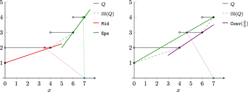
Notes. (Left panel) Example with continuous state space and incumbent (cyan dot). Core-point candidates (red and green dots) and associated LN Lagrangian cuts (red and green lines) obtained for heuristics Mid and Eps are highlighted. Dotted colored lines indicate the projection direction from the incumbent to . (Right panel) Same example but for Conv with , , and . The thick green dashed line highlights potential core points for different values of .
Despite their straightforwardness, these heuristics come with some notable challenges. The first two heuristics yield candidates satisfying . However, this choice is not necessarily feasible if integrality constraints are present (especially if ), leading to and preventing a reasonable choice for . Instead of evaluating , in such a case, we may revert to the value of the associated LP relaxation (LP-value), the current state component (epi-state), or the objective value at the incumbent (primal-obj). However, none of these approaches are guaranteed to yield core points. The heuristic Conv does not face this exact issue as it always considers convex combinations of objective values of feasible points. On the other hand, to be able to identify a good core point using this heuristic, it is first required to find a reasonable second feasible solution . This can be challenging in practice if relatively complete recourse is not satisfied or if . We provide a visualization of these challenges and improvement strategies in Online Appendix EC.4.
For these reasons, even with the proposed heuristics, we may end up with a normalized Lagrangian dual problem (11) that is unbounded. This is clearly unintended and should be detected in practice. We discuss strategies to do this in Online Appendix EC.5. Whenever (potential) unboundedness is detected, we may take some special countermeasures, such as artificially bounding the normalized Lagrangian dual problem (11) or resorting to strengthened Benders cuts instead of generating LN cuts.
4. Convergence Aspects
Given purely binary-state variables (i.e., for all ), the classical Lagrangian cuts from Zou et al. (2019) are valid, tight for at the incumbent , and finite (see Online Appendix EC.1). Therefore, they are sufficient to ensure (almost sure) finite convergence of SDDiP. Whereas they are always supporting according to Corollaries 1 and 2, deep and LN Lagrangian cuts are not necessarily tight at the incumbent, so these convergence results are not directly applicable. However, in this section, we show that under certain assumptions, the finite convergence results of SDDiP can still be established. For reasons of space, we do not present a complete, self-contained convergence proof but try to convey the key ideas.
4.1. Convergence for LN Cuts
For LN cuts, recall that according to Theorem 3, they are almost surely facet defining for (given that satisfies the conditions of case (ii) of Theorem 3). Additionally, is a convex polyhedron with finitely many facets (see Remark 4 and the formulation in Online Appendix EC.5). Therefore, if in all iterations (or at least at finite intervals of iterations), facet-defining LN cuts are generated, at most finitely many different cuts can be generated before is recovered completely. For the binary state space, this implies a tight approximation of at all . This is sufficient to obtain the known convergence results for SDDiP. For more technical details, we refer to Füllner (2024, chapter D.4).
4.2. Convergence for Deep Cuts
For deep Lagrangian cuts, proving convergence is a bit more intricate. The main idea, which is visualized in Online Appendix EC.2.9, is the following. Even if these cuts are not guaranteed to be tight at or facet defining, tight cuts will eventually be generated after finitely many steps. To show this, we use two key concepts. First, we consider subproblems with fixed approximations for all and all . In this case, the set remains constant over the iterations, so we drop its iteration index for simplicity. This assumption is satisfied for all leaf nodes in . All of the results that we derive for this case can then be extended to the whole scenario tree using induction. Second, we consider a subsequence of incumbents with fixed first component . If for all , then only finitely many different values can be attained by the state variables. Therefore, all of the results that we derive in this section can be extended to the whole state space by finite repetition.
For notational convenience, we set . We first obtain the following auxiliary result.
For any , consider a subsequence of incumbents with fixed first component for all . Then, the point and any sequence of solutions of the projection problems (12) satisfy .
We provide a proof in Online Appendix EC.2.10. Now, let K with denote the finite set of facets F of . Furthermore, let denote the subset of facets such that for all and for any , and analogously, let denote the subset of facets in which is contained. By definition of the points, and are nonempty. Intuitively, from Lemma 10, we can conclude that for sufficiently large , the points and are located on at least one joint facet and that can only be a vertex of if both points coincide. More precisely, we obtain the following result. For a detailed proof, we refer again to Füllner (2024, chapter D.4).
There exists some such that for all , we have . Moreover, there exists some such that for all , the point either is equal to or is not a vertex of .
Moreover, as also shown in Füllner (2024, chapter D.4), cuts supporting at a point in the relative interior of a face (or facet F) are also tight approximators at all other points at the same face (or facet). Therefore, because of Lemma 11, cuts supporting eventually will also support . With these auxiliary results, we are able to state the main tightness result, which we prove in Online Appendix EC.2.11.
For any , consider Subproblem (6) with fixed approximations for all . Moreover, consider a subsequence of trial points with fixed first component for all . Then, there exists some such that for all , a deep Lagrangian cut as defined in Definition 4 supports at .
We should emphasize that this worst-case reasoning of deep cuts eventually coinciding with classical Lagrangian cuts is solely used to show that (almost sure) finite convergence of SDDiP is still assured. In practice, the idea is that deep (as well as LN) Lagrangian cuts lead to stronger approximations outside of and thus, improve the computational performance.
5. Computational Experiments
We report results for a computational study of SDDiP incorporating the proposed cut-generation framework (Algorithm 1). For a detailed description of the SDDiP algorithm, we refer to Zou et al. (2019). We run SDDiP for two classes of MS-MILPs from the literature.
Capacitated lot-sizing problem (CLSP). A capacitated lot-sizing problem described in Trigeiro et al. (1989) with stagewise independent uncertain demand for each product. This problem is also considered in Ahmed et al. (2022) and identified to be challenging for exact decomposition methods, like SDDiP. We consider instances with 3 or 10 state variables; 4, 10, or 16 stages, and 20 realizations of the uncertain demand at each stage.
Capacitated facility location problem (CFLP). A capacitated facility location problem with stagewise independent uncertain facility disruptions (Seranilla and Löhndorf 2024). We consider an instance with 16 state variables, 100 stages, and 20 realization of the uncertainty at each stage.
With respect to the state space, it is important to mention that CLSP contains continuous state variables. For instances with three state variables, in order to ensure exactness of SDDiP, we thus apply a binary approximation of the state space using a discretization precision of 1.0; see Zou et al. (2019). This means that the modified MS-MILP, which is tackled by SDDiP, contains 30 state variables. We refer to this problem as CLSP-Bin. For instances with 10 state variables, using a binary approximation would produce state dimensions that are computationally intractable for SDDiP as its complexity grows exponentially in the dimension of the state space. Therefore, in these cases, we apply SDDiP to CLSP without a binary approximation and thus, without theoretical guarantees to close the optimality gap. In contrast, CFLP only contains binary state variables from the outset, so no binary approximation is required.
With respect to the uncertainty, for CLSP-Bin instances, we use the exact same scenarios as in Ahmed et al. (2022). For the larger instances (CLSP) that are not covered in that paper, we generate new scenarios using the same methodology. For CFLP, we use scenarios provided to us by Seranilla and Löhndorf (2024).
To assess the quality of the cuts obtained using our framework, we also run comparative tests using established cut-generation techniques in SDDiP. More precisely, we consider the following types of cuts.
B, SB, and L. Classical Benders cuts, strengthened Benders cuts (Zou et al. 2019), and Lagrangian cuts (Zou et al. 2019) (see Online Appendix EC.1), respectively, using a single-cut or multicut approach.
and . Deep Lagrangian cuts from Definition 4 for the -norm and the -norm, respectively.
LN. LN Lagrangian cuts from Definition 5 using the Mid, Eps, Relint, and Conv heuristics from Section 3.6 to identify core points and to determine the normalization coefficients.
The test cases and cut strategies are summarized in Table 3. By construction, all deep and LN cuts require using a multicut approach. For Eps, we use a perturbation of the incumbent toward by in each component. Conv is only considered for problem CFLP with binary state space as then, can be computed in a straightforward way; see Section 3.6. We use values of 0.5, 0.75, 0.9, and 0.99 for . Additionally, for problem CFLP, the risk of is prevalent in the search for core points because of the binary nature of the state space. Therefore, we use the objective value of the LP relaxation instead (LP-value), and we apply the strategy primal-obj to lift the -component of the core-point candidate as described in Section 3.6.
|
Table 3. Overview of Test Problems and Configuration of Experiments
| Problem | T | State space | Deep cuts | LN cuts | ||||||
|---|---|---|---|---|---|---|---|---|---|---|
| d | Orig. | Bin. App. | Approaches | Approaches | Unb. Check | Improv. | ||||
| CLSP-Bin | 4, 10, 16 | 20 | 3 (30) | Cont. | ✓ | , (MNC) | Mid, Eps, Relint | ✓ | — | |
| CLSP | 16 | 20 | 10 | Cont. | — | Mid, Eps, Relint | ✓ | — | ||
| CFLP | 100 | 20 | 16 | Bin. | — | X | Mid, Eps, Relint, Conv | ✓ | LP-value, primal-obj | |
Notes. The value for d in parentheses indicates dimension after binary approximation (Bin. App.). Bin., binary; Cont., continuous; Orig., original state space; Improv., improvement strategy if the subproblem is infeasible for candidate ; MNC, minimal norm choice is used; Unb. Check, check for unboundedness of Problem (11).
5.1. Implementation Details
SDDiP and all cut-generation approaches are implemented in Julia-1.9.3 (Bezanson et al. 2017) based on the existing packages SDDP.jl (Dowson and Kapelevich 2021) and JuMP.jl (Dunning et al. 2017). The code is available in GitHub (Füllner et al. 2026).
SDDiP is terminated after a predefined time limit or if the lower bounds do not improve considerably for 20 iterations. In each forward pass, one scenario path is randomly sampled. After termination of SDDiP, an in-sample Monte Carlo simulation with 1,000 replications is conducted on the finite scenario tree to compute a statistical upper bound (UB) for the obtained policy.
For LN cuts, the choice of normalization coefficients is crucial for the cut quality but also, to achieve a bounded dual problem. For all of the heuristics presented in Section 3.6, we may obtain an unbounded problem (11) if ; see Lemma 9. To detect a potentially insufficient choice of in advance, we use a (conservative) restriction of the problem (Figure EC.9 in Online Appendix EC.7) and use its infeasibility as a flag for possible unboundedness. This strategy is explained in more detail in Online Appendix EC.5. Given such a flag, we only generate an SB cut instead of an LN cut.
The Lagrangian dual problems in SDDiP are solved with a level bundle method (Lemaréchal et al. 1995), which can be considered as an enhancement of the Kelley method (Kelley 1960) (Online Appendix EC.6). Additionally, we bound the dual objective by . We run the method for a maximum of 1,000 (for CLSP) or 100 (for CFLP) iterations and an optimality tolerance of (for CLSP) or (for CFLP). The multipliers are initialized with a vector of zeros, and is initialized with one. If the level bundle method reports infeasibilities in the quadratic auxiliary problem, we proceed with a standard Kelley step instead. In the event of other numerical issues, a valid cut is constructed with the current values of the multipliers.
Additionally, in order to avoid numerical issues from the generated cuts, we apply some countermeasures.
We only add a new cut if the previous incumbent is cut away by at least .
We do not add a cut if , if , or if .
For CLSP-Bin and approach , some preliminary tests indicated a proneness to degeneracy of the dual problem and thus, cuts of bad quality. Therefore, for this case, we perform an additional optimization step where we minimize the -norm of among all optimal dual solutions (to which we restrict by fixing the dual objective value to ). This is indicated by MNC (minimal norm choice) in Table 3. This approach was previously proposed in SDDP.jl (Dowson and Kapelevich 2021). It is not applied for CLSP and CFLP.
All occurring LP, MILP, and quadratic subproblems are solved using Gurobi 9.0.3 with an optimality tolerance of and a time limit of 300 seconds. All tests are run on a Windows machine with 64 GB RAM and an Intel Core i7-7700K processor (4.2 GHz).
5.2. Results
For our first batch of experiments, we apply SDDiP with only one type of cut per run. The results are presented in Tables 4–6 and Online Appendix EC.7. The columns in Tables 4–6 contain the number of stages, the used cut-generation approach (Method), the best lower bound obtained (Best LB), a statistical upper bound computed after termination of SDDiP (Stat. UB; we report the upper limit of the computed confidence interval), the optimality gap (Gap), the number of iterations (# Iter.), the time in seconds (Time), the average time per iteration (Time/It), the average number of iterations (Avg. Lag-It) and the time (Time/Lag) required in the level bundle method to solve the Lagrangian dual, the average number of generated cuts per node (Cuts/Stage), and for LN cuts, the share of cases with detected potential unboundedness in the core-point identification process (Unb). In some cases, the simulation did not yield an upper bound estimate because of numerical issues.
|
Table 4. SDDiP Results for CLSP-Bin
| Stages | Method | Best LB | Stat. UB | Gap (%) | # Iter. | Time (seconds) | Time/It (seconds) | Avg. Lag-It | Time/Lag (seconds) | Cuts/ Stage | Unb (%) |
|---|---|---|---|---|---|---|---|---|---|---|---|
| 4 | Det. Equiv. | 1,503.0 | 1,542.3 | 3 | |||||||
| B (single) | 803.2 | 1,595.5 | 50 | 85 | 6 | 0 | — | — | 30 | — | |
| B (multi) | 804.5 | 1,602.6 | 50 | 59 | 5 | 0 | — | — | 86 | — | |
| SB (single) | 1,155.8 | 1,572.9 | 27 | 32 | 16 | 1 | — | — | 6 | — | |
| SB (multi) | 1,187.1 | 1,608.7 | 26 | 73 | 49 | 1 | — | — | 94 | — | |
| L (single) | 681.8 | 1,766.4 | 61 | 109 | lim | 99 | 49 | 1.6 | 109 | — | |
| L (multi) | 702.6 | 1,736.6 | 60 | 27 | lim | 404 | 51 | 6.6 | 540 | — | |
| -deep | 1,478.3 | 1,582.5 | 7 | 39 | lim | 272 | 67 | 4.7 | 704 | — | |
| -deep | 1,414.9 | 1,729.1 | 22 | 33 | lim | 331 | 133 | 5.5 | 621 | — | |
| LN-Mid | 1,496.6 | 1,579.0 | 5 | 36 | lim | 314 | 82 | 5.1 | 564 | 0 | |
| LN-Eps | 1,497.0 | 1,615.0 | 7 | 27 | lim | 412 | 115 | 6.8 | 483 | 0 | |
| LN-Relint | 1,500.9 | 1,623.3 | 8 | 33 | lim | 335 | 85 | 5.1 | 626 | 0 | |
| 16 | B (single) | 3,917.5 | 9,012.6 | 57 | 224 | 74 | 0 | — | — | 126 | — |
| B (multi) | 3,937.2 | 9,008.2 | 56 | 254 | 274 | 1 | — | — | 1,502 | — | |
| SB (single) | 5,913.7 | 8,673.6 | 32 | 194 | 493 | 3 | — | — | 44 | — | |
| SB (multi) | 6,030.2 | 8,676.8 | 31 | 585 | 9,252 | 16 | — | — | 1,679 | — | |
| L (single) | 607.4 | 9,524.5 | 94 | 63 | lim | 458 | 51 | 1.5 | 945 | — | |
| L (multi) | 651.6 | 9,444.7 | 93 | 19 | lim | 1,641 | 55 | 5.4 | 380 | — | |
| -deep | 3,547.5 | 9,756.3 | 64 | 42 | lim | 689 | 34 | 2.3 | 824 | — | |
| -deep | 3,707.1 | 9,708.3 | 62 | 33 | lim | 890 | 86 | 3.0 | 650 | — | |
| LN-Mid | 6,910.7 | 9,125.9 | 24 | 18 | lim | 1,784 | 117 | 5.8 | 352 | 0 | |
| LN-Eps | 6,067.6 | 9,164.6 | 34 | 15 | lim | 1,958 | 142 | 6.4 | 292 | 0 | |
| LN-Relint | 6,945.3 | 8,984.5 | 23 | 15 | lim | 1,951 | 122 | 6.4 | 291 | 0 | |
| SB + L (single) | 5,907.1 | 8,728.4 | 32 | 136 | lim | 213 | 47 | 0.8 | 157 | — | |
| SB + L (multi) | 5,922.0 | 8,750.8 | 32 | 52 | lim | 579 | 48 | 3.0 | 1,133 | — | |
| SB + -deep | 6,477.5 | 9,078.4 | 28 | 33 | lim | 907 | 90 | 7.5 | 643 | — | |
| SB + -deep | 6,220.9 | 8,968.8 | 31 | 24 | lim | 1,235 | 164 | 24.5 | 361 | — | |
| SB + LN-Mid | 6,615.9 | 9,003.1 | 27 | 29 | lim | 1,074 | 126 | 11.3 | 516 | 0 | |
| SB + LN-Eps | 6,705.0 | 8,947.8 | 25 | 29 | lim | 1,053 | 146 | 11.0 | 517 | 0 | |
| SB + LN-Relint | 6,832.1 | 9,071.4 | 25 | 29 | lim | 1,085 | 135 | 11.3 | 518 | 0 |
Notes. Time limits: : three hours (10,800 seconds); : eight hours (28,800 seconds). When the time limit is reached, this is indicated by lim. Det. Equiv refers to solving the deterministic equivalent of the MS-MILP. Bold values indicate best result among comparable runs. Avg. Lag-It, average number of iterations required in the level bundle method to solve the Lagrangian dual; Best LB, best lower bound obtained; Cuts/Stage, average number of generated cuts per node; Gap, optimality gap; # Iter., number of iterations; Method, used cut-generation approach; Stat. UB, statistical upper bound computed after termination of SDDiP; Time, time in seconds; Time/It, average time per iteration; Time/Lag, time required in the level bundle method to solve the Lagrangian dual; Unb, share of cases with detected potential unboundedness in the core-point identification process.
|
Table 5. SDDiP Results for CLSP with 10 State Variables
| Stages | Method | Best LB | Stat. UB | Gap (%) | # Iter. | Time (seconds) | Time/It (seconds) | Avg. Lag-It | Time/Lag (seconds) | Cuts/ Stage | Unb (%) |
|---|---|---|---|---|---|---|---|---|---|---|---|
| 16 | B (single) | 15,190 | 29,700 | 49 | 193 | 42 | 0 | — | — | 147 | — |
| B (multi) | 15,199 | 29,747 | 49 | 207 | 140 | 1 | — | — | 1,459 | — | |
| SB (single) | 20,373 | 29,600 | 31 | 111 | 189 | 2 | — | — | 42 | — | |
| SB (multi) | 21,045 | 29,343 | 28 | 281 | 2,459 | 9 | — | — | 987 | — | |
| L (single) | 14,440 | 32,429 | 56 | 93 | lim | 117 | 43 | 0.4 | 93 | — | |
| L (multi) | 19,689 | 31,468 | 37 | 30 | lim | 376 | 45 | 1.2 | 598 | — | |
| -deep | 23,678 | 30,064 | 21 | 36 | lim | 301 | 32 | 1.0 | 707 | — | |
| -deep | 23,610 | 30,333 | 22 | 30 | lim | 367 | 40 | 1.2 | 596 | — | |
| LN-Mid | 22,336 | 30,041 | 26 | 21 | lim | 543 | 90 | 1.8 | 411 | 0 | |
| LN-Eps | 22,296 | 30,340 | 27 | 25 | lim | 452 | 64 | 1.5 | 493 | 0 | |
| LN-Relint | 22,753 | 30,393 | 25 | 19 | lim | 595 | 99 | 2.0 | 375 | 3 | |
| SB + L (single) | 21,184 | 30,022 | 29 | 100 | lim | 110 | 42 | 0.4 | 147 | — | |
| SB + L (multi) | 22,431 | 30,257 | 26 | 39 | lim | 290 | 44 | 1.9 | 904 | — | |
| SB + -deep | 23,443 | 30,248 | 23 | 37 | lim | 309 | 51 | 2.2 | 807 | — | |
| SB + -deep | 23,424 | 30,062 | 22 | 36 | lim | 300 | 45 | 2.0 | 869 | — | |
| SB + LN-Mid | 23,036 | 30,161 | 24 | 31 | lim | 365 | 110 | 3.3 | 628 | 0 | |
| SB + LN-Eps | 23,195 | 30,086 | 23 | 34 | lim | 328 | 67 | 2.5 | 729 | 0 | |
| SB + LN-Relint | 23,038 | 30,371 | 24 | 31 | lim | 366 | 113 | 3.3 | 630 | 0 |
Notes. Time limits of three hours (10,800 seconds). Columns have the same meaning as for Table 4. When the time limit is reached, this is indicated by lim. Bold values indicate best result among comparable runs. Avg. Lag-It, average number of iterations required in the level bundle method to solve the Lagrangian dual; Best LB, best lower bound obtained; Cuts/Stage, average number of generated cuts per node; Gap, optimality gap; # Iter., number of iterations; Method, used cut-generation approach; Stat. UB, statistical upper bound computed after termination of SDDiP; Time, time in seconds; Time/It, average time per iteration; Time/Lag, time required in the level bundle method to solve the Lagrangian dual; Unb, share of cases with detected potential unboundedness in the core-point identification process.
|
Table 6. SDDiP Results for CFLP
| Stages | Method | Best LB | Stat. UB | Gap (%) | # Iter. | Time (seconds) | Time/It (seconds) | Avg. Lag-It | Time/Lag (seconds) | Cuts/ Stage | Unb (%) |
|---|---|---|---|---|---|---|---|---|---|---|---|
| 100 | B (single) | 59,744.4 | 78,498.9 | 24 | 592 | lim | 24 | — | — | 591 | — |
| B (multi) | 64,853.1 | — | — | 355 | lim | 41 | — | — | 7,026 | — | |
| SB (single) | 59,859.6 | 79,264.9 | 25 | 95 | lim | 153 | — | — | 95 | — | |
| SB (multi) | 63,127.0 | 78,737.6 | 20 | 90 | lim | 162 | — | — | 1,793 | — | |
| L (single) | 62,752.3 | 76,623.2 | 18 | 51 | lim | 294 | 2 | 0.1 | 43 | — | |
| L (multi) | 63,029.1 | 76,604.9 | 18 | 35 | lim | 425 | 2 | 0.1 | 677 | — | |
| -deep | 62,221.1 | 76,370.7 | 19 | 37 | lim | 405 | 2 | 0.1 | 737 | ||
| -deep | 61,919.9 | 76,267.9 | 19 | 23 | lim | 645 | 6 | 0.2 | 459 | ||
| LN-Mid | 74,103.0 | — | — | 9 | lim | 1,676 | 15 | 1.4 | 163 | 59 | |
| LN-Eps | 3,877.3 | — | — | 5 | lim | 2,880 | 21 | 1.4 | 100 | 0 | |
| LN-Relint | 72,405.3 | 76,461.9 | 5 | 15 | lim | 972 | 14 | 1.1 | 281 | 80 | |
| LN-Conv(50) | 75,013.0 | 75,461.9 | 1 | 8 | lim | 2,156 | 17 | 1.0 | 143 | 0 | |
| LN-Conv(75) | 75,185.5 | 75,448.3 | 0 | 7 | lim | 2,525 | 17 | 1.2 | 117 | 0 | |
| LN-Conv(90) | 72,666.0 | 76,288.0 | 5 | 9 | lim | 1,752 | 15 | 0.8 | 166 | 0 | |
| LN-Conv(99) | 5,579.4 | — | — | 15 | lim | 967 | 13 | 0.4 | 298 | 0 | |
| SB + L (single) | 63,444.8 | 77,722.2 | 18 | 49 | lim | 298 | 2 | 0.1 | 77 | — | |
| SB + L (multi) | 64,964.2 | — | — | 47 | lim | 314 | 2 | 0.1 | 1,437 | — | |
| SB + -deep | 64,664.6 | — | — | 36 | lim | 418 | 4 | 0.2 | 1,036 | — | |
| SB + -deep | 64,557.9 | — | — | 35 | lim | 426 | 24 | 0.3 | 998 | — | |
| SB + LN-Mid | 74,247.3 | 75,682.8 | 0 | 30 | lim | 490 | 15 | 1.1 | 717 | 81 | |
| SB + LN-Eps | 58,987.3 | 77,920.3 | 24 | 22 | lim | 681 | 24 | 0.3 | 480 | 0 | |
| SB + LN-Relint | 72,162.2 | 76,354.6 | 6 | 27 | lim | 544 | 14 | 1.5 | 670 | 83 | |
| SB + LN-Conv(50) | 75,206.8 | 75,442.3 | 0 | 25 | lim | 736 | 20 | 1.4 | 594 | 0 | |
| SB + LN-Conv(75) | 75,162.3 | — | — | 25 | lim | 729 | 18 | 1.3 | 563 | 0 | |
| SB + LN-Conv(90) | 73,831.0 | — | 25 | lim | 612 | 16 | 1.0 | 590 | 0 | ||
| SB + LN-Conv(99) | 59,517.5 | 77,437.5 | 23 | 25 | lim | 673 | 16 | 1.2 | 599 | 0 |
Notes. Time limits of four hours (14,400 seconds). Columns have the same meaning as for Table 4. Objective values are scaled by . When the time limit is reached, this is indicated by lim. Bold values indicate best result among comparable runs. Avg. Lag-It, average number of iterations required in the level bundle method to solve the Lagrangian dual; Best LB, best lower bound obtained; Cuts/Stage, average number of generated cuts per node; Gap, optimality gap; # Iter., number of iterations; Method, used cut-generation approach; Stat. UB, statistical upper bound computed after termination of SDDiP; Time, time in seconds; Time/It, average time per iteration; Time/Lag, time required in the level bundle method to solve the Lagrangian dual; Unb, share of cases with detected potential unboundedness in the core-point identification process.
5.2.1. CLSP-Bin.
In addition to Table 4, the development of the lower bounds obtained within SDDiP is illustrated in Figure 2 for CLSP-Bin. For , we can see that using deep or LN Lagrangian cuts, the LBs converge to the true optimal value. They clearly outperform the LBs obtained using approaches B, SB, and L, for which the bounds stall very fast and far away from optimality. In particular, despite the theoretical guarantees of the cuts, for L, the LBs improve very slowly for reasons outlined in Section 1.
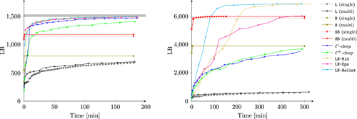
Notes. (Left panel) . (Right panel) . For , the shaded gray area is where the optimal value lies according to an approximate solution of the deterministic equivalent. For B and SB, SDDiP quickly terminates because of stalling lower bounds, so the last lower bound is interpolated over the whole time horizon. Marks are at every second iteration except for B and SB. LB, lower bound; min, minutes.
For larger T, we observe that LN cuts perform significantly better than deep cuts, which tend to be very flat; see Online Appendix EC.7. We also detect no unboundedness of the dual (11), so the core-point heuristics seem to work reasonably well. Again, using LN cuts, the LBs from B, SB, and L are outperformed. However, compared with SB, the difference gets smaller the more stages T are considered. This is mostly for computational reasons. As stated in Table 4, many fewer iterations are finished within the time limit because of the high computational cost of solving Lagrangian dual problems for each stage and iteration (see columns Avg. Lag-It and Time/Lag in Table 4 and also, see Online Appendix EC.7). Compared with single-cut approaches, the number of cuts per subproblem also grows more quickly, further slowing down the solution process.
The LBs give an indication of the direct effect that different types of cuts have on the outer approximation quality and the convergence behavior of SDDiP. However, in practice, what we are most interested in is the quality of the feasible policies obtained from running SDDiP (i.e., the statistical upper bounds computed after termination of SDDiP). In this regard, whereas using deep or LN cuts may considerably improve the solution quality compared with L, this is often not true compared with SB, where good feasible solutions seem to be identified quickly, and many more iterations are finished within the time limit.
5.2.2. CLSP.
For experiments on CLSP, we do not apply a binary approximation, and thus, we cannot expect the optimality gap to be closed. However, in return, iterations should take considerably less time.
In fact, we observe that the average iteration time is reduced considerably (by 60%–75%) compared with CLSP-Bin. For this reason and because the considered state space is lower dimensional, even without theoretical convergence guarantees, better optimality gaps are obtained for CLSP in the same time.
Again, the results show that deep and LN Lagrangian cuts manage to achieve better LBs and optimality gaps than conventional cuts as presented in Figure 3 and Table 5. Overall, deep cuts perform better as more iterations are finished in the same time. The results show that our proposed techniques for generating Lagrangian cuts may be helpful to improve the convergence behavior of SDDiP, even if no binary approximation is applied. However, as for the previous experiments, we cannot conclude that the improvement in lower bounds necessarily leads to an improvement of the in-sample performance of the obtained policy.
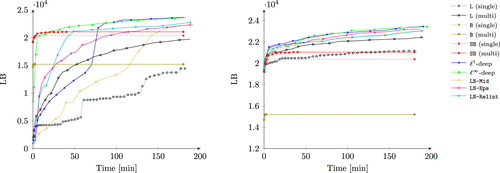
Notes. (Left panel) Runs with only one type of cuts. (Right panel) Runs with SB plus additional cuts starting from iteration 21. LB, lower bound; min, minutes.
5.2.3. CFLP.
For our experiments on CFLP, with binary state variables from the outset, the results are presented in Figure 4 and Table 6. The results differ considerably from those for the previous experiments.
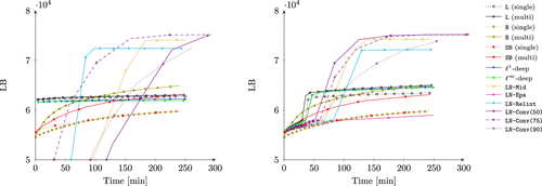
Notes. (Left panel) Runs with only one type of cuts. (Right panel) Runs with SB plus additional cuts starting from iteration 21. LB, lower bound; min, minutes.
First, we observe that all types of Lagrangian cuts lead to better UBs and thus, more feasible policies than SB. Interestingly, this is the case, although SB cuts are tight for this test problem. In reverse, deep cuts do not yield better LBs than B, SB, or L. This is mainly because deep cuts are completely flat, and thus, they lead to an unfavorable exploration of the state space (this also explains the small number of required iterations to solve the dual (11) to optimality). Concrete numbers to back these observations are provided in Online Appendix EC.7.
Second, for LN cuts, Eps yields tight cuts, but they seem to relate to very steep facets of the epigraph (again, see Online Appendix EC.7), so the obtained LBs are pretty bad. In contrast, Mid and Relint do not yield tight cuts on average. Additionally, for both, we observe the infeasibility challenges discussed in Section 3.6. They lead to (potentially) insufficient choices of , and thus, potential unboundedness of Problem (11) for more than 80% of the cases so that SB cuts are generated instead. Still, generating alternative cuts in only 15%–20% of the cases improves the LBs and UBs by a lot.
In general, LN cuts that use core points with relatively close to in early iterations (i.e., Mid, Conv(50), and Conv(75)) yield extremely good lower bounds in very few iterations and almost manage to close the optimality gap. According to Online Appendix EC.7, they seem to achieve a good trade-off between cut tightness at the incumbent and approximation quality everywhere else. Overall, the Conv heuristic leads to the best LBs and UBs without the infeasibility challenges that come along with Mid or Relint. The only drawback is that the average time spent for one iteration is extremely high.
5.3. Combination with Strengthened Benders Cuts
Using SDDiP with only Lagrangian cuts becomes extremely slow for large problems. Therefore, as already proposed in Zou et al. (2019), it is reasonable to combine them with cheaper cuts. In addition, the experiments for CLSP-Bin and CLSP indicate that using SB, it is often possible to quickly identify good feasible solutions but that the LBs may be too loose to get a certificate for optimality, whereas for our proposed Lagrangian cuts, it is the opposite. For these reasons, we consider a second batch of experiments where we start with only SB for the first 20 iterations to get a quick bound improvement and then, generate both SB cuts and Lagrangian cuts in each iteration. The results are presented in Figure 4 and Tables 4–6.
The LBs heavily improve for L but are not affected too much for deep or LN cuts. They are still better, however, than the ones obtained using only SB. As the simulated UBs are better than in the previous setting for all types of cuts, we conclude that a combination of SB cuts and Lagrangian cuts may be helpful to identify good policies early while not compromising good LBs and convergence guarantees.
5.4. Discussion and Potential Improvements
Overall, our results show significant improvements of the obtained LBs and UBs using the proposed cut-generation framework compared with standard Lagrangian cuts from Zou et al. (2019). In the light of challenges (b) and (c) presented in Section 1, this confirms that either better tight cuts or nontight cuts that improve the exploration of the state space are generated. For problem CFLP, the proposed LN cuts manage to approximately close the optimality gap, which is by far not the case for conventional cuts.
As advice for practitioners, it seems that deep cuts, which are often relatively flat, are most valuable for problems with large (initially continuous) state spaces as they are less costly to generate than LN cuts, which usually yield better LBs. LN cuts are more prone to numerical issues and require more tuning (e.g., with regard to the core-point heuristics). Among deep cuts, using the -norm seems most promising.
For (initially) continuous state spaces, using the heuristics Mid, Relint, and Eps yields very good LBs, with Mid looking like the most reliable and easy to implement approach. Also, almost no cases of potential unboundedness of the dual (11) are detected. This confirms that these heuristics work reasonably well for these types of problems. For problems with binary state spaces, however, infeasibility issues significantly aggravate the identification of (good) core points. In contrast, the Conv heuristic is tailor made for these problems. Under relatively complete recourse, it only requires one additional evaluation of to compute a proven core point. As shown for CFLP, this strategy can be costly but can lead to very good results.
Whereas deep and LN variants outperform classical Lagrangian cuts, this is not necessarily true for SB cuts. For CLSP-Bin and CLSP, SB cuts yield worse LBs but better feasible policies at termination. Given their cheap computation, this means that SB cuts should remain the first choice for many practical problems, especially if SDDiP has to be stopped prematurely. If they do not close the optimality gap sufficiently, they may be combined with our proposed cuts to find a good balance between improving LBs and UBs.
We should acknowledge that our proposed framework does not necessarily lead to a reduced time spent on generating Lagrangian cuts. It may even be increased because of the requirement of using a multicut approach. Hence, challenge (a) from Section 1 remains. In the future, this could be addressed in several ways. First, cut-selection schemes, where the number of cuts is kept at a minimum, could be explored. Second, parallelization, warm-starting, or acceleration techniques for the Lagrangian dual could be explored. Third, a smart restriction of the dual feasible space (see Chen and Luedtke 2022) may help to reduce the computational effort for solving Lagrangian dual problems while not compromising cut quality by too much. Finally, it might be of interest to investigate potential extensions of the proposed framework to a single-cut approach.
6. Conclusion
In this article, we show how Lagrangian cuts can be generated by solving special normalized Lagrangian dual problems when solving MS-MILPs. We prove that different normalizations lead to cuts with different properties. This allows for a lot of flexibility and notably, extends the toolbox for cut generation in SDDiP.
We provide computational results for experiments on two known test problems. They show that lower bounds and also, sometimes upper bounds obtained in SDDiP can be vastly improved. However, other known drawbacks of SDDiP persist, such as excessive computational effort, slow convergence, and inability to close the optimality gap for large problem instances. Therefore, more research on cut selection, cut combination schemes, or dual space restrictions is required to allow for an extensive application in practice.
Finally, it should be possible to extend the proposed framework to cases where Lagrangian duals are solved to generate nonconvex cuts; see, for instance, Füllner and Rebennack (2022) and Füllner et al. (2024).
The authors thank Filipe Cabral, Bonn Kleiford Seranilla, and Nils Löhndorf for providing data for the computational experiments.
References
- (2022) Stochastic Lipschitz dynamic programming. Math. Programming 191:755–793.Crossref, Google Scholar
- (1964) On the generalized transportation problem. Management Sci. 11(1):188–202.Link, Google Scholar
- (2026) Integer L-shaped and Lagrangian cuts revisited: A unified perspective. Oper. Res. Lett. 66:107427.Crossref, Google Scholar
- (1962) Partitioning procedures for solving mixed-variables programming problems. Numerische Mathematik 4(1):238–252.Crossref, Google Scholar
- (2017) Julia: A fresh approach to numerical computing. SIAM Rev. 59(1):65–98.Crossref, Google Scholar
- (2021) Refined cut selection for Benders decomposition: Applied to network capacity expansion problems. Math. Methods Oper. Res. 94:383–412.Crossref, Google Scholar
- (2010) Computing deep facet-defining disjunctive cuts for mixed-integer programming. Math. Programming 122:197–223.Crossref, Google Scholar
- (2022) On generating Lagrangian cuts for two-stage stochastic integer programs. INFORMS J. Comput. 34(4):2332–2349.Link, Google Scholar
- (2019) “Facet” separation with one linear program. Math. Programming 178:361–380.Crossref, Google Scholar
- (2006) A convex-analysis perspective on disjunctive cuts. Math. Programming 106:567–586.Crossref, Google Scholar
- (2024) On the ReLU Lagrangian cuts for stochastic mixed integer programming, Preprint, submitted November 9, https://arxiv.org/abs/2411.01229.Google Scholar
- (2021) SDDP.jl: A Julia package for stochastic dual dynamic programming. INFORMS J. Comput. 33(1):27–33.Link, Google Scholar
- (2017) JuMP: A modeling language for mathematical optimization. SIAM Rev. 59(2):295–320.Crossref, Google Scholar
- (2010) A note on the selection of Benders’ cuts. Math. Programming 124:175–182.Crossref, Google Scholar
- (2024) On approximating non-convex value functions in stochastic dual dynamic programming and related decomposition methods. PhD thesis, Karlsruher Institut für Technologie, Karlsruhe, Germany.Google Scholar
- (2022) Non-convex nested Benders decomposition. Math. Programming 196:987–1024.Crossref, Google Scholar
- (2024) On Lipschitz regularization and Lagrangian cuts in multistage stochastic mixed-integer linear programming. Preprint, submitted August 7, https://optimization-online.org/?p=27295.Google Scholar
- (2026) Generating Lagrangian cuts using normalized dual problems in multistage stochastic mixed-integer programming. https://doi.org/10.1287/ijoc.2024.1039.cd, https://github.com/INFORMSJoC/2024.1039.Google Scholar
- (2026) A novel Pareto-optimal cut selection strategy for Benders decomposition. Math. Programming Comput. 18:211–257.Crossref, Google Scholar
- (2025) Deepest cuts for Benders decomposition. Oper. Res. 73(5):2591–2609.Link, Google Scholar
- (1960) The cutting-plane method for solving convex programs. J. Soc. Indust. Appl. Math. 8(4):703–712.Crossref, Google Scholar
- (1995) New variants of bundle methods. Math. Programming 69(1–3):111–147.Crossref, Google Scholar
- (1981) Accelerating benders decomposition: Algorithmic enhancement and model selection criteria. Oper. Res. 29(3):464–484.Link, Google Scholar
- (2008) Practical enhancements to the Magnanti–Wong method. Oper. Res. Lett. 36:444–449.Crossref, Google Scholar
- (1991) Multi-stage stochastic optimization applied to energy planning. Math. Programming 52(1–3):359–375.Crossref, Google Scholar
- (2020) The Benders dual decomposition method. Oper. Res. 68(3):878–895.Link, Google Scholar
- (2022) A closest Benders cut selection scheme for accelerating the Benders decomposition algorithm. INFORMS J. Comput. 34(5):2804–2827.Link, Google Scholar
- (2024) Multistage stochastic facility location under facility disruption uncertainty. Preprint, submitted May 13, https://optimization-online.org/?p=26395.Google Scholar
- (2013) On generating maximal nondominated Benders cuts. Ann. Oper. Res. 210:57–72.Crossref, Google Scholar
- (2019) On the mathematics of energy system optimization. PhD thesis, TU München, Munich, Germany.Google Scholar
- (1989) Capacitated lot sizing with setup times. Management Sci. 35(3):353–366.Link, Google Scholar
- (2019) Stochastic dual dynamic integer programming. Math. Programming 175:461–502.Crossref, Google Scholar

