
Optimizing the Sunday Singles Lineup for a Ryder Cup Captain
Abstract
The Ryder Cup competition between Team USA and Team Europe is the premier team event in professional golf, largely because of the drama associated with head-to-head matches on the final day (Sunday). The captain of each team must determine the exact sequence of his 12 golfers in the 12 Sunday singles matches, and neither captain is precisely aware of the other captain's intended lineup. Because the losing captain has often been criticized for choosing what the critics deem to be a poor lineup, we develop a quantitative methodology that a captain can use to determine his Sunday singles lineup to maximize the probability that his team is in possession of the Ryder Cup upon completion of the competition. As part of our effort, we develop a statistical model for estimating the three possible outcomes (win, lose, tie) of each singles match. Using the 1989–2008 Ryder Cup competitions as examples, we find that using our statistical model within our methodology indicates that the Sunday singles competition is not greatly impacted by the lineup selected by the captain. However, we define another example that indicates our methodology can be of great benefit if a player's performance is affected by who his singles match opponent is.
The Ryder Cup is a biannual golf competition that pits a team (side) of 12 male professional golfers from the United States (Team USA) against a team (side) of 12 male professional golfers from Europe (Team Europe). A captain leads each side; the two captains are famous professional golfers who have played in multiple previous Ryder Cup competitions. Over the years, the Ryder Cup has become one of the most highly anticipated professional golf events, largely because of the caliber of the 24 golfers and the drama associated with the competition.
Each Ryder Cup competition takes place over three days and includes 28 18-hole golf matches. On the morning of the first day (Friday), the captain of each side selects eight of his golfers to compete in teams of two in four four-ball matches against two-man teams from the other side. In a four-ball match, each player plays his own ball on every hole. A team's score on a hole is the lower of the two teammates' scores. On the afternoon of the first day, the captain of each side selects eight of his golfers to compete in teams of two in four sets of foursomes matches against two-man teams from the other side. In a foursomes (alternate-shot) match, the two players on a team take turns hitting shots until each hole is completed. Furthermore, they alternate who hits the first shot on each hole (one teammate hits the first shot on the odd-numbered holes; the other teammate hits the first shot on the even-numbered holes). The format of the second day (Saturday) is identical to that of the first day. In each of the four sets of four matches on the first two days, the captain of each side chooses his four teams and their sequence (i.e., which team plays in the first match, which team plays in the second match, etc.) with no knowledge of the intentions of the other captain.
On the final day (Sunday), each golfer competes in 1 of 12 head-to-head (one golfer from Team USA against one golfer from Team Europe) singles matches. Upon conclusion of Saturday's matches, each captain must submit a lineup of his golfers that indicates who will play in Sunday's first match, who will play in Sunday's second match, etc. As with the first two days, each captain prepares his Sunday singles lineup with no knowledge of the intentions of the other captain.
All the matches in the Ryder Cup are played under the rules of match play. Accordingly, each of the 18 holes in each match is treated as a separate competition; that is, each hole is won, lost, or halved (tied). The team (in a four-ball or foursomes match) or individual (in a singles match) who wins the most holes wins the match. If the competitors in a match win the same number of holes, then the match is halved (tied).
In a Ryder Cup competition, if a match is won, then the winning team (individual) earns a point for their (his) side. If a match is halved, then each side receives half a point. Because there are 28 matches, a side wins the competition and possession of the Ryder Cup (the trophy received by the winning team) if its members earn 14.5 or more points. If the competition ends in a 14–14 tie, then the side in possession of the Ryder Cup from the previous competition retains the cup.
The Scrutiny on Sunday Singles
The sides in the Ryder Cup are typically evenly matched; therefore, it has often been a close competition that is decided by a dramatic set of Sunday matches. Because 12 of the 28 Ryder Cup points are available on Sunday, the possibility exists for significant comebacks by the side trailing after two days of play. In the 1999 Ryder Cup, Team Europe led 10–6 after two days. The Team USA captain, Ben Crenshaw, made the bold decision to front-load his Sunday singles lineup; he placed his six best golfers in the first six matches, hoping to create momentum early in the day. Team USA earned 8.5 points on Sunday to win the competition.
When the Ryder Cup is decided by a small margin, the losing captain is often criticized for his Sunday singles lineup (criticism of the losing captain's Friday and Saturday decisions is rare). In the 2002 Ryder Cup, the two sides were tied after two days. The consensus among golf experts was that Team USA had better individual golfers and therefore held a significant advantage on Sunday. Accordingly, the Team Europe captain, Sam Torrance, adopted the front-loading strategy used by Crenshaw in 1999. The Team USA captain, Curtis Strange, took the opposite (back-loading) approach. His reasoning was that he wanted his two best golfers, Tiger Woods and Phil Mickelson, to play in the matches at the end of the day, because he expected those matches to ultimately determine the winner. Team Europe won 4.5 points in the first six Sunday matches, and after only 10 singles matches, Team Europe had secured enough points to win the Ryder Cup. Strange claimed to be dumbfounded by the Team Europe lineup, saying (Reilly 2002), “I've never seen somebody front-load like this.” This statement sparked tremendous criticism, as evidenced by the following comments (Reilly 2002).
Uh, hello? Curtis? Loading the front is exactly how Ben Crenshaw pulled off the Miracle at Brookline in 1999. (Rick Reilly, Sports Illustrated).
We couldn't have handpicked a better draw for us today. When we saw the draw, everyone knew we were going to win. (Jesper Parnevik, Team Europe golfer).
Applying Operations Research to the Sunday Singles
Because Ryder Cup captains are often criticized for their Sunday lineup decisions, our interest is in using quantitative modeling to assist these captains with preparing their Sunday singles lineup (we leave the analysis of Friday and Saturday decision making for future work). Only Hurley (2002, 2007, 2009) has used quantitative analysis in the study of Ryder Cup singles matches.
Hurley (2002, p. 74) argues that an optimal course of action for a Ryder Cup captain is to prepare his Sunday singles lineup by “drawing names from a hat.” This argument is based on game theory and the assumption that the golfers participating in the Ryder Cup are not affected by their position in the lineup (we maintain this assumption in our work).
Hurley (2007) argues in support of Curtis Strange's decision to put Tiger Woods in the final singles match of the 2002 Ryder Cup. Hurley uses some statistics and hole-by-hole Monte Carlo simulation to argue that (1) there is no evidence of a momentum effect in the results of past Ryder Cup Sunday singles matches (accordingly, we do not consider a momentum effect), and (2) the most likely conclusion of the 2002 Ryder Cup was that the outcome would not be decided until the final match. Although the analysis in this paper is not as formal as in Hurley (2002), he does assume that the 24 golfers competing in the Ryder Cup are homogeneous and that their performance is not affected by their position in the Sunday singles lineup. Under these assumptions, Hurley (2009) estimates that a comeback of the type observed in the 1999 Ryder Cup will occur, on average, once every 125 years.
In the following sections, we develop and analyze a quantitative methodology that can be used by a Ryder Cup captain in preparing his Sunday singles lineup. In developing our methodology, we propose a statistical model for estimating the three possible outcomes of an 18-hole singles match between two well-known male professional golfers.
The Methodology
We develop our methodology from the perspective of the Team USA captain and, unlike Hurley (2002), we assume that the Team Europe captain is using a prespecified approach to determine his lineup. Like Hurley (2002), we assume that the outcome of the 12 Sunday singles matches depends only on who plays in each match (the order of the matches is irrelevant) and that these 12 matches are statistically independent.
In our methodology, each Team USA golfer is assigned a number such that the golfers are numbered in descending order of skill level (player 1 is Team USA's best player; player 12 is Team USA's worst player). Each Team Europe golfer is assigned a number in a similar manner—these golfers are also numbered in descending order of skill level. Each match is assigned a number based on the order in which matches are played.
To optimize his Sunday singles lineup, the Team USA captain needs information about how the Team Europe captain plans to construct his lineup. There are 12! feasible Sunday singles lineups available to the Team Europe captain, and we assume that the probability that the Team Europe captain selects each of these potential lineups is known by the TEAM USA captain. These probabilities can then be used to compute the probability that each Team Europe golfer is assigned to each match.
To optimize his Sunday singles lineup, the Team USA captain also needs information about how each of his golfers would perform against each of Team Europe's golfers. We accomplish this by specifying the probabilities that each of the 144 potential matchups would result in a Team USA victory or a halved match.
Based on this information, the Team USA captain must determine the assignment of his golfers to the 12 matches. We use binary assignment variables to model these decisions, and we constrain the combinations of these decision variables such that exactly one Team USA golfer plays in each singles match and each Team USA golfer is assigned to exactly one match.
To compare feasible assignments (lineups), we assume that the Team USA captain intends to maximize the probability that his team wins the Ryder Cup. Henceforward, we define “wins the Ryder Cup” to mean that Team USA is in possession of the Ryder Cup upon completion of the competition. For any feasible Team USA lineup, we can use the specified probabilities of each Team Europe lineup and the probabilities of the three outcomes of each potential matchup to compute the probability of each of the 312 realizations (for each match, the possibilities are: USA wins, USA loses, match is halved) of the Sunday singles matches. Because each realization implies a certain number of points earned by Team USA, we can then compute the probability mass function of the number of points earned by Team USA on Sunday. Depending on the number of points that Team USA earns on Friday and Saturday, we can then compute the probability that it earns enough points on Sunday to win the Ryder Cup.
Unfortunately, the logic involved in computing the probability mass function of the points earned by Team USA on Sunday renders the probability that Team USA wins the Ryder Cup intractable. Because there are 12! feasible Team USA lineups, using total enumeration to find the optimal team lineup is computationally prohibitive. This challenge is analogous to the challenge faced by Cassady et al. (2005) in optimizing the ranking of National Collegiate Athletic Association (NCAA) college football teams. Therefore, we use the same heuristic approach that Cassady et al. (2005) used to find a ranking to recommend a Sunday singles lineup.
The heuristic designed by Cassady et al. (2005) is a two-step process that begins with a genetic algorithm (GA). The first generation of the GA is created randomly, and all subsequent generations are created by culling, breeding, and mutating solutions from the previous generation. The GA provides no guarantee of optimality; therefore, the solution it recommends is subjected to a local search heuristic that consists of attempting all possible pairwise switches within the recommended lineup (and restarting the local search when a switch improves the solution).
In our implementation of the heuristic designed by Cassady et al. (2005), we use the same culling, breeding, and mutation parameters that they recommend. In the GA, we evaluate 100 generations, with each generation containing 100 solutions. Like Cassady et al. (2005), because the first generation of the GA is generated randomly, we replicate the entire heuristic 20 times. The best solution found during these 20 replications is our recommended lineup.
Modeling Match Probabilities
To use our methodology, the Team USA captain must be able to specify the probabilities of the three outcomes (the Team USA golfer wins, the Team USA golfer loses, the match is halved) for each of the 144 potential Sunday singles matches. The captain could estimate these probabilities based on his own experiences, beliefs, and intuition. However, that information is not available to us; therefore, we define our own method to generate these probabilities. When we have discussed this research project in the past, one approach that others often suggest is to use casino betting lines to establish these probabilities. Unfortunately, these betting lines are not generated for hypothetical matches; therefore, they do not exist until the Sunday singles lineups have been selected. In addition, betting lines are intended to equally split the wagers on each outcome—not to predict the outcome of a match—thus leading to betting lines changing over time. Therefore, casino betting lines are not useful to us.
Our approach is to create a statistical model for estimating the probabilities of the three outcomes of a hypothetical 18-hole singles match between two well-known male professional golfers. Building such a model requires some type of quantitative measure of a golfer's ability. The most widely accepted quantitative evaluation of a professional golfer's skill level is the World Golf Ranking, which is updated on a weekly basis and is often used for comparing the performance of professional golfers. These rankings are based on golfer performance on each of the six professional golf tours (a tour is a series of competitive events) that are included in the International Federation of Professional Golfers' Association (PGA) Tours.
The World Golf Ranking ranks golfers in descending order of a numerical score called average points. Each golfer's average points is based on his performance in events on the six professional tours during the previous two years. Each event (on each tour) held during these two years is allocated a certain number of points, which is based on when the event was played (more recent events receive more points) and who played in the event (more highly ranked golfers in the event implies more points). The points for each event are allocated to the golfers who played in the event based on how they performed (a better finish implies more points). A golfer's average points is the average number of points per event that he earned over the past two years (the divisor in average points is set to 30 if the golfer played fewer than 30 events during the two years). The World Golf Ranking (http://www.officialworldgolfranking.com) publishes the top 10 golfers (see Table 1).
|

Table 1 Professional golfers are assigned points for each event in which they participated over the most recent two-year period. The World Golf Ranking ranks golfers in descending order based on golfers' average points per event. The golfers listed are the top 10 golfers in the World Golf Ranking as of April 11, 2010.
| World rank | Golfer | Total points | Number of events | Average points |
|---|---|---|---|---|
| 1 | Tiger Woods | 496.81 | 40 | 11.75 |
| 2 | Phil Mickelson | 394.35 | 43 | 9.17 |
| 3 | Steve Stricker | 338.90 | 43 | 7.88 |
| 4 | Lee Westwood | 399.99 | 51 | 7.84 |
| 5 | Ian Poulter | 308.30 | 50 | 6.17 |
| 6 | Jim Furyk | 287.58 | 47 | 6.12 |
| 7 | Paul Casey | 268.29 | 44 | 6.10 |
| 8 | Ernie Els | 331.14 | 55 | 6.02 |
| 9 | Martin Kaymer | 272.92 | 52 | 5.25 |
| 10 | Anthony Kim | 259.51 | 52 | 4.99 |
The largest value of average points in the history of the World Golf Raking is 32.44, the value achieved by Tiger Woods on June 3, 2001. The difference in the average points of golfers in adjacent ranking positions decreases as one moves down through the rankings. Over the last 10 years, the average difference in average points between the golfers ranked 1 and 2 is approximately seven, whereas the average difference in average points between those ranked 50 and 100 is less than one.
Although subjected to a lot of criticism over the years, the World Golf Ranking is the only quantitative system that is used for determining who gets to play in some of golf's most prestigious events, including all four major championships (The Masters, the U.S. Open, the Open Championship, the PGA Championship). Therefore, we use a golfer's World Golf Ranking average points at the time of the match of interest as a quantitative measure of a golfer's ability.
To build our statistical model for estimating the probabilities of the three outcomes of a singles match, we collected data only from events sanctioned by the International Federation of PGA Tours that include 18-hole singles matches, and we collected data only from those events that took place since the inception of the World Golf Ranking. Our database includes all Ryder Cup singles matches from 1989–2008, all Presidents Cup singles matches from 1994–2009, and all World Golf Championship (WGC) Match Play Championship 18-hole matches from 1999–2010. The Presidents Cup is a biannual golf tournament that has a similar format to the Ryder Cup; the Presidents Cup slates a team from the United States versus a team from the rest of the world, excluding Europe. The WGC Match Play Championship is a 64-golfer single-elimination tournament featuring the world's top 64 golfers (as determined by the World Golf Ranking); every match in the tournament is an 18-hole singles match except for the match between the final two golfers (which is a 36-hole singles match). Because matches in the WGC Match Play Championship cannot end in a tie (extra holes are played if necessary), we list any match from that tournament that required more than 18 holes as a tie (to be consistent with the format of the Ryder Cup Sunday singles). Our data collection effort resulted in a database of 920 18-hole singles matches. Each record in the database contains the higher-ranked golfer's World Golf Ranking average points, the lower-ranked golfer's World Golf Ranking average points, and the outcome of the match with respect to the higher-ranked golfer.
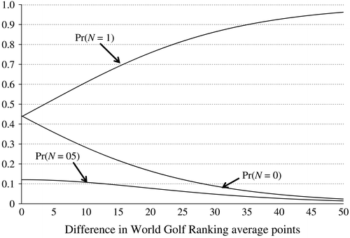
Our methodology requires estimated probabilities of three ordered categorical responses (higher-ranked golfer loses, match is halved, higher-ranked golfer wins). Therefore, we use ordered logistic regression to model the probabilities of the three match outcomes as a function of the difference between the World Golf Ranking average points of the two golfers. The appendix includes the details associated with the construction of this statistical model; Figure 1 provides a graphical summary of the behavior of these models.
This model has several attractive and intuitive characteristics:
For any given value of the difference in the World Golf Ranking average points of the two golfers, the three probabilities sum to 1.
The probability that the higher-ranked golfer wins is increasing and approaches 1 as the difference in the two golfers' skill levels increases.
The probability that the higher-ranked golfer loses is decreasing and approaches 0 as the difference in the two golfers' skill levels increases.
The probability that the match is halved is decreasing and approaches 0 as the difference in the two golfers' skill levels increases.
In a match between two golfers of almost equal ability, the two golfers have a near equal chance of winning the match.
Modeling the Behavior of the Opposing Captain
To use our methodology, the Team USA captain also must be able to specify the probability that the Team Europe captain places each of his golfers in each of the 12 positions in the Sunday singles lineups. These probabilities could be estimated by the Team USA captain based on his own experiences, beliefs, and intuition. However, because that information is not available to us, we define three scenarios to capture examples of these probabilities.
Our three hypothetical scenarios are based on approaches used by past Ryder Cup captains. Our first scenario, scenario F, is intended to mimic front-loading—the captain sequences his golfers in roughly descending order of ability. In creating scenario F, we did not limit our attention to perfect front-loading (the best Team Europe golfer is assigned to the first match, the second-best Team Europe golfer is assigned to the second match, etc.). Instead, we assume that the best golfers are more likely to be placed near the front of the lineup and that the worst golfers are more likely to be placed near the end of the lineup. Our second scenario, scenario B, is intended to mimic back-loading. Because back-loading is the opposite of front-loading, we model scenario B as the opposite of scenario F. Table 2 details the probabilities of each golfer match assignment under scenarios F and B.
|
Table 2 The golfer match-assignment probabilities under scenario F (front-loading) demonstrate the intention to place the best golfers near the front of the lineup and the worst golfers near the end of the lineup. These probabilities under scenario B (back-loading) demonstrate the intention to place the best golfers near the end of the lineup and the worst golfers near the front of the lineup. The Team Europe golfers are numbered in decreasing order of ability.
| Team Europe golfer | |||||||||||||
|---|---|---|---|---|---|---|---|---|---|---|---|---|---|
| Scenario | Match (%) | ||||||||||||
| F | B | 1 | 2 | 3 | 4 | 5 | 6 | 7 | 8 | 9 | 10 | 11 | 12 |
| 1 | 12 | 18.75 | 18.75 | 18.75 | 18.75 | 6.25 | 6.25 | 6.25 | 6.25 | 0 | 0 | 0 | 0 |
| 2 | 11 | 18.75 | 18.75 | 18.75 | 18.75 | 6.25 | 6.25 | 6.25 | 6.25 | 0 | 0 | 0 | 0 |
| 3 | 10 | 18.75 | 18.75 | 18.75 | 18.75 | 6.25 | 6.25 | 6.25 | 6.25 | 0 | 0 | 0 | 0 |
| 4 | 9 | 18.75 | 18.75 | 18.75 | 18.75 | 6.25 | 6.25 | 6.25 | 6.25 | 0 | 0 | 0 | 0 |
| 5 | 8 | 6.25 | 6.25 | 6.25 | 6.25 | 12.50 | 12.50 | 12.50 | 12.50 | 6.25 | 6.25 | 6.25 | 6.25 |
| 6 | 7 | 6.25 | 6.25 | 6.25 | 6.25 | 12.50 | 12.50 | 12.50 | 12.50 | 6.25 | 6.25 | 6.25 | 6.25 |
| 7 | 6 | 6.25 | 6.25 | 6.25 | 6.25 | 12.50 | 12.50 | 12.50 | 12.50 | 6.25 | 6.25 | 6.25 | 6.25 |
| 8 | 5 | 6.25 | 6.25 | 6.25 | 6.25 | 12.50 | 12.50 | 12.50 | 12.50 | 6.25 | 6.25 | 6.25 | 6.25 |
| 9 | 4 | 0 | 0 | 0 | 0 | 6.25 | 6.25 | 6.25 | 6.25 | 18.75 | 18.75 | 18.75 | 18.75 |
| 10 | 3 | 0 | 0 | 0 | 0 | 6.25 | 6.25 | 6.25 | 6.25 | 18.75 | 18.75 | 18.75 | 18.75 |
| 11 | 2 | 0 | 0 | 0 | 0 | 6.25 | 6.25 | 6.25 | 6.25 | 18.75 | 18.75 | 18.75 | 18.75 |
| 12 | 1 | 0 | 0 | 0 | 0 | 6.25 | 6.25 | 6.25 | 6.25 | 18.75 | 18.75 | 18.75 | 18.75 |
Our third scenario, scenario A, represents the hypothetical case in which the Team USA captain somehow knows exactly how the Team Europe captain intends to construct his Sunday singles lineup. Under scenario A, the Sunday singles lineup decisions reduce to deciding which Team USA player should play against each Team Europe player (because the order of the matches is assumed to have no impact on the players).
Analysis of the 2002 Ryder Cup
Because of the criticism aimed at 2002 Team USA Ryder Cup captain Curtis Strange for his Sunday singles lineup decisions, we use the 2002 Ryder Cup to demonstrate our methodology (see Table 3).
|
Table 3 These 24 golfers participated in the 2002 Ryder Cup. The golfer's World Golf Ranking average points at the time of the 2002 Ryder Cup accompanies each name.
| Golfer | Team USA golfer | Team USA golfer average points | Team Europe golfer | Team Europe golfer average points |
|---|---|---|---|---|
| 1 | Tiger Woods | 18.19 | Sergio Garcia | 6.68 |
| 2 | Phil Mickelson | 9.30 | Padraig Harrington | 5.32 |
| 3 | David Toms | 5.86 | Colin Montgomerie | 4.02 |
| 4 | Davis Love III | 5.45 | Darren Clarke | 3.91 |
| 5 | Jim Furyk | 4.83 | Bernhard Langer | 3.46 |
| 6 | David Duval | 4.63 | Niclas Fasth | 3.12 |
| 7 | Scott Verplank | 3.40 | Thomas Bjorn | 3.08 |
| 8 | Scott Hoch | 3.34 | Jesper Parnevik | 2.20 |
| 9 | Mark Calcavecchia | 2.65 | Paul McGinley | 1.97 |
| 10 | Paul Azinger | 2.42 | Pierre Fulke | 1.78 |
| 11 | Stewart Cink | 2.22 | Phillip Price | 1.36 |
| 12 | Hal Sutton | 1.30 | Lee Westwood | 1.08 |
Entering the final day of the 2002 competition, Team USA needed only 6 of the 12 available points in Sunday singles to win the Ryder Cup. The World Golf Ranking average points (see Table 3) reflect the consensus among golf fans and the media that Team USA had a significant advantage in individual match play. Table 4 contains the estimated probability (based on our statistical model) that Team USA would win or halve each of the 144 hypothetical Sunday singles matchups; to use our statistical model to construct Table 4, we must note which player in each hypothetical matchup is the higher-ranked player (see Table 4).
|
Table 4 Our statistical model permits the estimation of the possible outcomes of each of the 144 hypothetical Sunday singles matches for the 2002 Ryder Cup. The top number in each cell corresponds to the estimated probability of a Team USA victory; the bottom number in each cell corresponds to the probability of a halved match.
| Team USA golfer | Team Europe golfer (%) | |||||||||||
|---|---|---|---|---|---|---|---|---|---|---|---|---|
| 1 | 2 | 3 | 4 | 5 | 6 | 7 | 8 | 9 | 10 | 11 | 12 | |
| 1 | 63 | 66 | 68 | 68 | 68 | 69 | 69 | 70 | 71 | 71 | 72 | 72 |
| 10 | 10 | 10 | 10 | 9 | 9 | 9 | 9 | 9 | 9 | 9 | 9 | |
| 2 | 48 | 51 | 53 | 53 | 54 | 55 | 55 | 56 | 56 | 57 | 58 | 58 |
| 12 | 12 | 12 | 12 | 12 | 12 | 12 | 11 | 11 | 11 | 11 | 11 | |
| 3 | 43 | 45 | 47 | 47 | 48 | 49 | 49 | 50 | 51 | 51 | 52 | 52 |
| 12 | 12 | 12 | 12 | 12 | 12 | 12 | 12 | 12 | 12 | 12 | 12 | |
| 4 | 42 | 44 | 46 | 46 | 47 | 48 | 48 | 49 | 50 | 50 | 51 | 51 |
| 12 | 12 | 12 | 12 | 12 | 12 | 12 | 12 | 12 | 12 | 12 | 12 | |
| 5 | 41 | 43 | 45 | 45 | 46 | 47 | 47 | 48 | 49 | 49 | 50 | 50 |
| 12 | 12 | 12 | 12 | 12 | 12 | 12 | 12 | 12 | 12 | 12 | 12 | |
| 6 | 41 | 43 | 45 | 45 | 46 | 46 | 46 | 48 | 48 | 49 | 49 | 50 |
| 12 | 12 | 12 | 12 | 12 | 12 | 12 | 12 | 12 | 12 | 12 | 12 | |
| 7 | 39 | 41 | 43 | 43 | 44 | 44 | 44 | 46 | 46 | 47 | 47 | 48 |
| 12 | 12 | 12 | 12 | 12 | 12 | 12 | 12 | 12 | 12 | 12 | 12 | |
| 8 | 38 | 41 | 43 | 43 | 44 | 44 | 44 | 46 | 45 | 47 | 47 | 48 |
| 12 | 12 | 12 | 12 | 12 | 12 | 12 | 12 | 12 | 12 | 12 | 12 | |
| 9 | 37 | 40 | 42 | 42 | 43 | 43 | 43 | 45 | 45 | 45 | 46 | 47 |
| 12 | 12 | 12 | 12 | 12 | 12 | 12 | 12 | 12 | 12 | 12 | 12 | |
| 10 | 37 | 39 | 41 | 42 | 42 | 43 | 43 | 44 | 45 | 45 | 46 | 46 |
| 12 | 12 | 12 | 12 | 12 | 12 | 12 | 12 | 12 | 12 | 12 | 12 | |
| 11 | 37 | 39 | 41 | 41 | 42 | 43 | 43 | 44 | 44 | 45 | 45 | 46 |
| 12 | 12 | 12 | 12 | 12 | 12 | 12 | 12 | 12 | 12 | 12 | 12 | |
| 12 | 35 | 37 | 40 | 41 | 40 | 41 | 41 | 43 | 43 | 43 | 44 | 44 |
| 12 | 12 | 12 | 12 | 12 | 12 | 12 | 12 | 12 | 12 | 12 | 12 | |
Table 5 contains the actual 2002 Ryder Cup Sunday singles lineups submitted by Team USA captain, Curtis Strange, and Team Europe captain, Sam Torrance.
|
Table 5 The actual Sunday singles lineups from the 2002 Ryder Cup can be used to produce estimates of the probabilities of the three outcomes of each match from the final day of the 2002 Ryder Cup.
| Match | Team USA golfer | Team Europe golfer | Probability of a Team USA win (%) | Probability of a halve (%) | Match result |
|---|---|---|---|---|---|
| 1 | 8 | 3 | 43 | 12 | USA loss |
| 2 | 3 | 1 | 43 | 12 | USA win |
| 3 | 6 | 4 | 45 | 12 | Halve |
| 4 | 12 | 5 | 40 | 12 | USA loss |
| 5 | 9 | 2 | 40 | 12 | USA loss |
| 6 | 11 | 7 | 43 | 12 | USA loss |
| 7 | 7 | 12 | 48 | 12 | USA win |
| 8 | 10 | 6 | 12 | 43 | Halve |
| 9 | 5 | 9 | 49 | 12 | Halve |
| 10 | 4 | 10 | 50 | 12 | Halve |
| 11 | 2 | 11 | 58 | 11 | USA loss |
| 12 | 1 | 8 | 70 | 9 | Halve |
The strategy employed by Curtis Strange is very similar to our scenario B (back-loading), and the strategy employed by Sam Torrance is consistent with our scenario F (front-loading). Table 5 also contains the estimated probability that Team USA would win or halve each of these 12 matches, as well as the actual outcome of each match.
Based on these matchups, our assumptions, and our statistical model, Figure 2 contains the probability mass function of the points earned by Team USA on Sunday of the 2002 Ryder Cup.
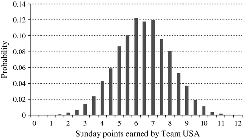
Based on these probabilities, Team USA had a 66.2 percent probability of earning the six or more points needed to win the Ryder Cup. In the actual competition, Team USA only earned 4.5 Sunday points. Our probability mass function indicates that the probability of Team USA earning 4.5 points or less was only 15.0 percent. Therefore, we suggest that its loss in the 2002 Ryder Cup was a low-probability event corresponding to a combination of poor play by Team USA and excellent play by Team Europe.
To gain insight into what Curtis Strange should have done, we implemented our methodology for the 2002 Ryder Cup using all three of our hypothetical scenarios. Table 6 provides the recommended Team USA lineup for each scenario and several opportunities for discussion.
|
Table 6 The actual Sunday singles lineup used by Team USA during the 2002 Ryder Cup differs from the lineups suggested by our methodology for each of the three scenarios.
| Match | Actual Team USA lineup | Recommended Team USA lineup | ||
|---|---|---|---|---|
| Scenario F | Scenario B | Scenario A | ||
| 1 | 8 | 8 | 5 | 1 |
| 2 | 3 | 1 | 4 | 6 |
| 3 | 6 | 11 | 6 | 11 |
| 4 | 12 | 7 | 3 | 8 |
| 5 | 9 | 9 | 10 | 7 |
| 6 | 11 | 10 | 9 | 10 |
| 7 | 7 | 2 | 12 | 9 |
| 8 | 10 | 12 | 2 | 2 |
| 9 | 5 | 4 | 7 | 12 |
| 10 | 4 | 5 | 8 | 3 |
| 11 | 2 | 6 | 11 | 4 |
| 12 | 1 | 3 | 1 | 5 |
| Probability of Team USA winning the Ryder Cup | 66.3% | 66.3% | 66.5% | |
For example, the recommended lineups for scenarios F and B provide the same probability of Team USA retaining the Ryder Cup (because scenario B is the inverse of scenario F). A key observation to make is that the recommended lineup for scenario A, as compared to the lineup used by Curtis Strange, provides only a 0.3 percent gain in the probability of Team USA winning the Ryder Cup.
After making note of the similarity of the performance of the actual Team USA lineup and the recommended lineup for scenario A, we modified our methodology to minimize the probability of Team USA winning the Ryder Cup. In other words, our revised methodology aims to find the worst Team USA lineup. The bold cells in Table 7 provide a comparison of the performance resulting from the original and revised methodologies.
|
Table 7 Applying our statistical model and methodology to all Ryder Cup competitions during the period 1989--2008 implies that the Sunday singles lineup is not a major factor in the likelihood of Team USA winning the competition.
| Year | Probability of Team USA winning the Ryder Cup (%) | |||
|---|---|---|---|---|
| Scenario A | Scenario F or B | |||
| Best lineup | Worst lineup | Best lineup | Worst lineup | |
| 1989 | 28.7 | 27.9 | 28.7 | 28.3 |
| 1991 | 40.4 | 39.9 | 40.3 | 40.1 |
| 1993 | 43.2 | 42.1 | 42.8 | 42.5 |
| 1995 | 78.6 | 77.9 | 78.3 | 77.9 |
| 1997 | 8.5 | 8.3 | 8.5 | 8.4 |
| 1999 | 16.7 | 15.9 | 16.5 | 16.1 |
| 2002 | 66.5 | 65.8 | 66.3 | 66.0 |
| 2004 | 3.5 | 3.4 | 3.5 | 3.4 |
| 2006 | 11.2 | 10.7 | 11.1 | 10.8 |
| 2008 | 67.0 | 66.6 | 66.9 | 66.8 |
The results make it clear that, according to our methodology and statistical model, manipulating the Sunday singles lineup has little impact on the probability of Team USA winning the Ryder Cup.
To determine if the 2002 results are representative of most Ryder Cup competitions, we implemented the original (maximize probability of winning) and revised (minimize probability of winning) methodologies for the 10 Ryder Cup competitions held during 1989–2008. Table 7 summarizes the results of these experiments and demonstrates that our 2002 results are representative.
Commentary
Our results for the 1989–2008 Ryder Cup competitions lead us to the same key conclusion as Hurley (2002): because golfers in the Ryder Cup are evenly matched, it is difficult for a captain to gain a meaningful advantage in Sunday singles by optimizing his Sunday singles lineup. Hurley (2002) assumed that both captains act optimally in preparing Sunday singles lineups, and thus was able to support his game-theoretic conclusion with a formal proof. We reached the same conclusion using an optimization methodology that assumes that only one captain acts optimally and uses a statistical model of match outcomes that is based on historical match-play data.
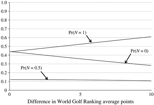
The minor differences in performance between our recommended Sunday singles lineup and other feasible lineups are because of the behavior implied by our statistical model of individual match outcomes. To improve a feasible lineup, the captain must interchange golfers in the lineup. For example, Curtis Strange might have elected to place Tiger Woods in the first match in 2002. Doing so would have required that Scott Hoch be placed somewhere else in the lineup. Suppose Curtis Strange elected to simply swap Woods and Hoch in the lineup. Making this swap increases Team USA's probability of winning the first match from 43 percent to 68 percent. However, Team USA's probability of winning the 12th match drops from 70 percent to 46 percent; therefore, the overall probability of Team USA winning the Ryder Cup only increases to 66.3 percent. As Figure 3 demonstrates, the similarity in the magnitude of changes resulting from interchanging golfers in the lineup is because our statistical model of match outcomes exhibits approximately linear behavior in the range typically observed in Ryder Cup matches.
Our statistical model of match outcomes is based on the assumption that a player's World Golf Ranking average points is the sole descriptor of his ability. As a result, the transitive property applies to comparisons among the competing golfers. As a final step in our analysis, we consider the question: what if this transitivity does not hold? In other words, what if the Team USA captain believes that each of his players has different capabilities, depending on who his Sunday opponent is?
To address this question, we generated probabilities (see Table 8) for each potential 2002 matchup so that the transitive property does not hold.
|
Table 8 If the probabilities associated with match outcomes indicate that player performance is affected by the opponent, then the Team USA captain can exploit this to his advantage. Boldface indicates the most favorable matchups for Team USA in the 2002 Ryder Cup for such a scenario.
| Team USA golfer | Team Europe golfer (%) | |||||||||||
|---|---|---|---|---|---|---|---|---|---|---|---|---|
| 1 | 2 | 3 | 4 | 5 | 6 | 7 | 8 | 9 | 10 | 11 | 12 | |
| 1 | 25 | 59 | 45 | 49 | 23 | 21 | 44 | 69 | 42 | 25 | 60 | 42 |
| 12 | 12 | 12 | 12 | 12 | 12 | 12 | 12 | 12 | 12 | 12 | 12 | |
| 2 | 46 | 70 | 28 | 62 | 46 | 79 | 77 | 60 | 67 | 67 | 46 | 57 |
| 12 | 12 | 12 | 12 | 12 | 12 | 12 | 12 | 12 | 12 | 12 | 12 | |
| 3 | 31 | 59 | 44 | 68 | 70 | 20 | 54 | 25 | 46 | 30 | 38 | 73 |
| 12 | 12 | 12 | 12 | 12 | 12 | 12 | 12 | 12 | 12 | 12 | 12 | |
| 4 | 75 | 42 | 51 | 58 | 32 | 27 | 63 | 27 | 67 | 44 | 79 | 38 |
| 12 | 12 | 12 | 12 | 12 | 12 | 12 | 12 | 12 | 12 | 12 | 12 | |
| 5 | 34 | 39 | 22 | 54 | 42 | 32 | 35 | 66 | 69 | 43 | 68 | 56 |
| 12 | 12 | 12 | 12 | 12 | 12 | 12 | 12 | 12 | 12 | 12 | 12 | |
| 6 | 41 | 48 | 46 | 31 | 74 | 71 | 50 | 31 | 54 | 78 | 66 | 20 |
| 12 | 12 | 12 | 12 | 12 | 12 | 12 | 12 | 12 | 12 | 12 | 12 | |
| 7 | 72 | 75 | 69 | 59 | 62 | 61 | 51 | 48 | 54 | 35 | 30 | 54 |
| 12 | 12 | 12 | 12 | 12 | 12 | 12 | 12 | 12 | 12 | 12 | 12 | |
| 8 | 63 | 25 | 26 | 61 | 27 | 40 | 58 | 31 | 78 | 41 | 48 | 41 |
| 12 | 12 | 12 | 12 | 12 | 12 | 12 | 12 | 12 | 12 | 12 | 12 | |
| 9 | 76 | 47 | 67 | 32 | 21 | 48 | 54 | 76 | 30 | 33 | 54 | 74 |
| 12 | 12 | 12 | 12 | 12 | 12 | 12 | 12 | 12 | 12 | 12 | 12 | |
| 10 | 36 | 61 | 70 | 80 | 63 | 58 | 30 | 78 | 46 | 76 | 47 | 57 |
| 12 | 12 | 12 | 12 | 12 | 12 | 12 | 12 | 12 | 12 | 12 | 12 | |
| 11 | 23 | 52 | 26 | 63 | 75 | 60 | 61 | 73 | 52 | 34 | 63 | 67 |
| 12 | 12 | 12 | 12 | 12 | 12 | 12 | 12 | 12 | 12 | 12 | 12 | |
| 12 | 66 | 73 | 51 | 49 | 62 | 30 | 46 | 25 | 29 | 49 | 23 | 44 |
| 12 | 12 | 12 | 12 | 12 | 12 | 12 | 12 | 12 | 12 | 12 | 12 | |
For example, Team USA player 3 has a 28 percent greater chance of defeating Team Europe player 2 than Team Europe player 1; however, Team USA player 4 has a 33 percent lesser chance of defeating Team Europe player 2 than Team Europe player 1. We implemented our methodologies (best lineup and worst lineup) using these probabilities for scenarios A and F. Under scenario A, the recommended Team USA lineup results in a probability of 99.6 percent that Team USA wins the Ryder Cup, and the worst-case lineup results in a probability of 12.7 percent that Team USA wins the Ryder Cup. The bold cells in Table 8 indicate the matchups associated with our recommended lineup for scenario A. These recommendations clearly exploit the matchups that are favorable for each individual Team USA player. For scenario F, the recommended Team USA lineup results in a probability of 82.6 percent that Team USA wins the Ryder Cup, and the worst-case lineup results in a probability of 62.1 percent that Team USA wins the Ryder Cup. Therefore, a captain who believes that his players' performance is impacted by who their opponent is can potentially benefit greatly from applying our methodology particularly if he has insight into the specific plan of the opposing captain.
As a final note, we believe that our methodology could be extended for even greater potential if we saw evidence that players are impacted by their position in the lineup. Unfortunately, because professional golf events of this type only occur once per year, the data to support the modeling associated with these extensions are scarce at best.
Appendix. The Statistical Model of Match Outcomes
Because our methodology requires estimated probabilities of winning, losing, and halving a match, we develop a statistical model that estimates the match outcome as a function of the difference between the average points of the two golfers. We use the most common statistical model of ordered categories—ordered logistic regression (McCullagh 1980).
Ordered logistic regression is theoretically appropriate to estimate the relationship between an ordinal dependent variable and other independent variables. Our dependent variable is categorical and ordered (win, halve, or loss), and our lone independent variable is δ, the difference between the World Golf Ranking average points of the higher-ranked and lower-ranked golfer. Therefore, in our case, ordered logistic regression uses maximum likelihood to estimate cut-points, κ1 and κ2, and a basic score that is a simple linear function of δ. Let N = 1 if the higher-ranked golfer wins the match, let N = 0 if the higher-ranked golfer loses the match, and let N = 0.5 if the match is halved. The probability of observing a certain match outcome is equal to the probability that the functional value is within a range of relevant cut-points:
In keeping with a direct generalization of traditional logistic regression, we assume that u has the logistic distribution, and find match outcome probabilities to be
According to an ordered logistic regression model of our data, the maximum-likelihood estimate of β is 0.06948 and is assumed to be normally distributed. The standard error (0.02070) is such that we reject the null hypothesis that β = 0; the model is not just theoretically appropriate, but also by most standards statistically significant (standard normal test statistic of 3.36; p-value of approximately 0.001). The cut-points are estimated to be κ1 = −0.2374 and κ2 = 0.2484. Furthermore, the model chi-square goodness-of-fit statistic (with one degree of freedom) is 12.06 (p-value of approximately 0.0005). Accordingly, we reject the assumption of independence between the match outcome and the independent variable.
Ordered logistic regression is also known as the proportional odds model because, with respect to cumulative probabilities, the ratio of odds corresponding to pairs of covariate values should be independent of category and depend only on the difference between the covariate values. To lend further credibility to our statistical model, an approximate likelihood-ratio test of proportional odds across response categories does not seriously challenge the proportional odds assumption (p-value of the test is 0.6438).
References
- (2005) Ranking sports teams: A customizable quadratic assignment approach. Interfaces 35(6) 497–510.Link, Google Scholar
- (2002) How should team captains order golfers on the final day of the Ryder Cup matches? Interfaces 32(2) 74–77.Link, Google Scholar
- (2007) The 2001 Ryder Cup: Was Strange's strategy to put Tiger Woods in the anchor match a good one? Decision Anal. 4(1) 41–45.Link, Google Scholar
- (2009) Calculating the odds of the miracle at Brookline. Chance 22(4) 36–38.Crossref, Google Scholar
- (1980) Regression models for ordinal data (with discussion). J. Royal Statist. Soc. Ser. B 42(2) 109–142.Google Scholar
- (2002) Uneasy Ryder. . Accessed May 1, 2010, http://sportsillustrated.cnn.com/inside_game/magazine/life_of_reilly/news/2002/10/01/life_of_reilly/.Google Scholar

