
Implementation of Continuous Flow in the Cabinet Process at the Schneider Electric Plant in Tlaxcala, Mexico
Abstract
This work presents the development and improvements obtained by the implementation of continuous flow in the cabinet process at Schneider Electric’s manufacturing plant in Tlaxcala, Mexico. The areas involved were the demand-planning, materials-planning, and manufacturing processes and warehouse operations. The implementation process, which consisted of shared planning, analysis of control operations, and synchronization of lean manufacturing techniques, led to increased communication among personnel within departments at the Schneider Tlaxcala plant (STP). In addition, this implementation produced the following benefits: (1) improvement of demand coverage in high-demand seasons without exceeding the production capacity, (2) reduction of shortages and delays in the assembly line with associated savings of approximately $3.5 million, (3) reduction of 17.5% in the overproduction of stamped parts and thus on the daily holding inventory, (4) setup time reduction of 77%, and (5) elimination of product flow between the cabinet process and the warehouse to reduce delivery lead time to the assembly line. The fifth benefit was made possible because STP was able to supply the cabinets directly to the assembly line in two days. As a result, the company released 49 storage spaces and improved its customer service by 5% because it could make the final products available to customers at the appropriate time (i.e., on schedule). After 24 months, these improvements led to total recurring savings of approximately $1 million considering an investment of 1.25%. In addition, Schneider Electric was able to successfully replicate this methodology in similar manufacturing plants in North America.
Schneider Electric S.A. de C.V. (Schneider) is a global company specializing in energy management and automation. In Mexico, Schneider has more than 8,000 employees distributed throughout 10 manufacturing plants. We performed this study in the Schneider Tlaxcala plant (STP).
STP has nine assembly lines that produce more than 7,000 models of finished products. The company manufactures the products using a large variety of subassemblies, which can be supplied externally or manufactured in-house. The breakers and cabinets are safety subassemblies; thus, they are manufactured internally.
In this study, we focused on the air conditioner (AC) disconnect assembly line, which produces diverse finished products using a common standard security subassembly. This subassembly is produced using the cabinet process. Our analyses of this process detected substandard planning, which resulted in expensive disruptions to the system. To provide a holistic decision support solution, the objective of this study was to implement a pilot of continuous flow in the cabinet process.
Currently, STP managers must often make business decisions using limited information because the corporate offices, which manage the information, are located in the United States. The corporate offices develop a strategic aggregate plan every six months and then distribute it to each plant in North and Central America.
As a consequence of this poor planning, STP had a major problem: the AC disconnect assembly line stopped or encountered a delay when demand increased substantially. According to STP’s records, from July 2011 to September 2014, this assembly line encountered 12 line stoppages that lasted an average of four days and 67 delays of approximately five hours each because of lack of components. Its finance department estimated that a nonproductive hour costs $2,378; therefore, the total cost of these line stoppages and delays was approximately $3,536,086.00.
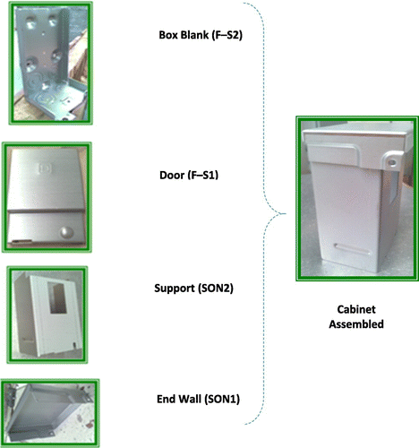
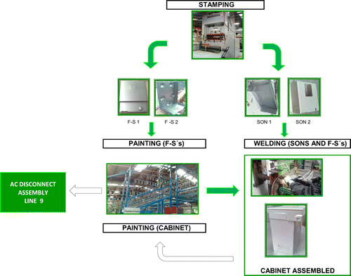
This problem was caused by a capacity production constraint in the cabinet process, which prevented the necessary number of components from reaching the appropriate subassembly. The cabinet process consists of manufacturing and assembling all the components that comprise a cabinet, and the operations involved in this process are stamping, welding, painting, and assembling. Figure 1 presents the components of a cabinet.
As a result, STP compensated for the shortage of raw materials and subassemblies by generating a high safety stock. However, this caused other problems, including scarcity of warehouse space and high holding costs. Poor planning also resulted in the need for constant adjustments to increase (or reduce) capacities in the work centers to try to satisfy changes in demand, and long setup times for the core machines.
Therefore, STP’s objective was to coordinate the demand-planning, materials-planning, and manufacturing processes and warehouse operations to improve manufacturing performance. By involving many management levels and enhancing a company’s collaborative decision-making process, it is possible to provide a clear understanding of how diverse decisions and actions can impact performance metrics, and how it can change policies and set targets for the overall benefit of the company (Katircioglu et al. 2014).
Literature Review
Competitiveness in the globalized world highlights the importance of increasing the efficiency of a company’s operations and administrative processes. Frequently, business decisions are made with insufficient information and a greater or lesser degree of uncertainty, depending on the time and resources available for researching and analyzing information.
Many techniques, philosophies, and methodologies have been developed to address accurate decision making. The literature includes some traditional textbooks and papers focused on these topics. Examples include Chase et al. (2000), Everett and Ronald (2001), Ballou (2004), Heizer and Render (2004), Hanke and Wichern (2009), and Carrizo and Campos (2011).
Within this context, demand planning is the most important process in any company because of its key role in production efficiency. It determines the capacity planning resources that a company must acquire in advance (Álvarez-Socarrás et al. 2013).
One of the most important techniques for business decision making is forecasting, which supports corporate planning in the short, medium, and long terms, depending on the objectives of the strategy (Franses 2004, Wallace 2006). It provides the foundation for planning budgets, materials, and human resources. Therefore, forecasting supports the control of costs in specific periods. In practice, using a method that generates minimum forecasting errors is critical (Armstrong 2001, Everett and Ronald 2001).
To determine the best production plan, it is necessary to verify inventory levels and production and budgeting capacities under different scenarios (Thomas and Bollapragada 2010). Consequently, determining the most appropriate trade-offs is also important because capacity-related decisions affect service levels and return on investment. For example, an excess of capacity increases fixed costs and the risk of equipment obsolescence; shortages in capacity may result in customer complaints and loss of customers (Álvarez-Socarrás et al. 2013). The results obtained from aggregate planning lead to a more detailed master production program, which serves as the basis for task programming and material delivery (Heizer and Render 2004).
Other key aspects of production efficiency include reducing various types of waste and improving process performance. These benefits can be achieved by implementing continuous flow using lean manufacturing techniques, such as single-minute exchange of die (SMED) and just-in-time (JIT) inventory strategies (Vokurka and Rhonda 2000).
SMED can reduce nonproductive time by streamlining and standardizing tool change operations using simple techniques (Carrizo and Campos 2011, Adanna and Shantharam 2013). SMED has been widely used to reduce wasted time resulting from tool changes, and it has proven to be an effective approach to address stoppage time (Samuel et al. 2013). The objective of JIT is to ensure that all resources are used efficiently by eliminating everything that does not contribute value to the customer (Swamidass 2000). JIT can improve company performance by reducing inventory levels (Lacerda et al. 2012).
In addition, lean initiatives are frequently used to make improvements on the control floor. However, they are necessary to understanding the context of the problem, and evaluating the appropriateness of these initiatives is critical because potential pitfalls may occur because of misapplication (Gorman et al. 2009).
Many researchers have successfully documented the savings associated with integrated decision making for logistical planning (Çetinkaya et al. 2009). Thomas and Bollapragada (2010), Manary et al. (2009), and Olavson and Fry (2008) present similar case studies in which they analyze the various areas in a company in integrated ways.
Similarly, a continuous flow in the cabinet process can be developed by considering an integrated framework of demand forecasting, capacity planning, and inventory levels. STP implemented a well-defined and planned business-improvement program to eliminate further waste.
In this paper, we present the details of the implementation of continuous flow to improve the processes at STP and discuss the proposed changes, the results obtained, our conclusions, and future work.
Details of the Current Conditions at STP
In this section, we present details of the current conditions and underlying problems of the STP areas involved in the case study.
Demand Planning
The main activities of STP’s demand-planning department are to analyze the variability between the received forecast and (1) the release of production customer orders, which are final-assembly schedule orders, (2) the backorders, and (3) the actual sales equivalent to five weeks of sales. These activities are performed to monitor the inventory levels, the capacity of the lines, and the economic order quantity (EOQ) rates. This result is an updated plan for the quantities of finished products to be produced monthly.
Other departments, such as materials planning, manufacturing, and warehouse operations use this updated plan to perform their monthly planning and to adjust their resources based on customer requirements.
An important point to mention is that the department responsible for demand forecasting is located in the corporate offices. It performs a six-month demand-forecasting process using a simple linear regression method and distributes the forecast to STP’s demand-planning department. However, this forecast is unreliable because STP receives only the forecast; it does not receive any information allowing it to adjust the forecast. Thus, high error rates result.
Materials Planning
STP’s materials-planning department uses the forecast, which the demand-planning department has entered into the enterprise resource planning (ERP) system. The forecast of finished products is analyzed by material analysts who determine the relationship between a particular parent and a particular component; thus, the finished products are segmented into their different subassemblies, components, and raw materials by a materials hierarchical structure called the bill of materials. This segmentation provides clear information about when and how many materials should be ordered from external suppliers and in-house production to complete the assembly of the final product on time.
Currently, the requirements are requested based on the forecasted monthly demand. By analyzing the history of the forecasted demand for the sales generated in the previous 39 months, we found a forecast error higher than 20% in the previous 12 months. These errors caused the following problems:
shortages of raw materials and subassemblies in the production lines when demand increases;
excess of raw materials for the manufacturing of subassemblies when demand is low;
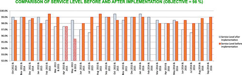
an average service level that is lower than the target service level in 17 of the 39 months (Figure 2).
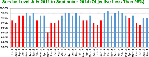
Notes. These records are from July 2011 to September 2014. The darker columns represent the months in which the service level was below 98%.
Specifically, these problems caused STP to hold a large inventory (i.e., a 10-day inventory of approximately 15,375 pieces) of stamped parts, which are manufactured as part of the cabinet process. As a consequence, this inventory generated significant holding costs; because of demand fluctuations, STP held safety stock of up to 100% to ensure customer delivery.
Manufacturing Process
The AC disconnect assembly line uses a 15% make-to-order manufacturing process, including a cell-process layout and a batch-production process. In this environment, the company does not hold an inventory of finished product: each customer order is assembled as needed using standard configuration options and components. The remaining 85% use a make-to-stock manufacturing process, with a production-process layout and a mass-production process. In this environment, the production is done in batches; therefore, STP maintains an inventory of each model of finished product. The subassemblies produced in-house are handled using the kanban (KB) system, a manufacturing system in which the component supply is controlled by using an instruction card that is sent through the production line and that many companies use successfully.
The KB system works synchronously, determining the most suitable inventory levels and production lead times of the required products throughout each stage of the manufacturing process for both in-house production and external suppliers (Mukhopadhyay and Shanker 2005, Wan and Chen 2007). The KB system is also called a card system because, in its simplest implementation, it uses cards that (1) are placed on containers of materials and (2) are removed when these containers are used; this is done to ensure the replacement of such materials. Thus, the cards act as a verification in the production process. More sophisticated implementations use the same philosophy, replacing the cards by other methods of flow visualization. The KB system is considered a subsystem of a JIT inventory strategy (Duri et al. 2000).
However, as we mention above, the constant adjustments in production levels frequently caused the STP KB system to crash. STP made these adjustments because the many variations between the forecasted and the actual demand significantly affected its manufacturing processes. In the cabinet process, which consists of stamping, welding, painting, and assembling operations, the critical operation is stamping, because the stamping machines manufacture all stamped parts for all production lines. Thus, these machines manufacture stamped parts for both the cabinets that are supplied to the AC disconnect assembly line and for other styles of cabinets that are supplied to the other lines.
Hence, the forecasting errors caused the following problems in this manufacturing process:
Constant adjustments were required to increase or reduce the capacities of the work centers.
The necessity to adjust the numbers of operations personnel resulted in additional training costs for personnel hired when monthly demand increased; for example, an increase of 25%–40% between December 2013 and March 2014 required STP to hire six workers at a training cost of $4,800.
Setup times for the stamping machines and the production runs were both long; for example, the adjustment time for each tool change was over 39 minutes.
Constant adjustments in production levels frequently resulted in the loss of KB cards; as a result, the KB system often crashed because of cards not being requested.
Warehouse Operations
One of the responsibilities of the warehouse is to temporarily store the stamped parts that will be used to assemble the cabinet. The father and son components F–S1, F–S2, SON1, and SON2 comprise the cabinet (Figure 1). When each component is required for an operation, it is stored temporarily in the warehouse. In Figure 3, we show that this process includes four unnecessary storage steps before the cabinet is assembled, and one unnecessary storage step before the components are delivered as a subassembly to the AC disconnect assembly line.
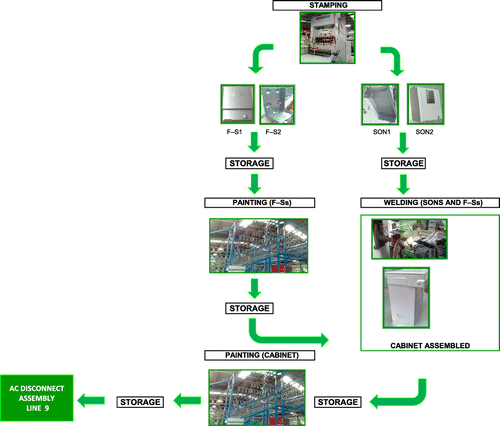
Note. The flow of the four components that comprise the finished cabinet shows that the components are stored unnecessarily five times—four times prior to cabinet assembly and once prior to delivery to the AC disconnect assembly line.
The F–S1 and F–S2 components are stored twice before being used in the cabinet. The SON1 and SON2 components are stored at least once before being assembled as part of the cabinet. These components, along with F–S1 and F–S2, are then sent to the manufacturing cells, which represent a subset of JIT manufacturing and lean manufacturing that encompasses group technology. The goal of cellular manufacturing is to produce a wide variety of similar products as quickly as possible, while generating as little waste as possible. Here, the aforementioned components are welded to produce the assembled cabinets, and these subassemblies are stored twice more before finally being sent to the AC disconnect assembly line.
It is important to mention that the batch sizes of these components are disproportionate as a result of unfit planning. The consumption must have a one-to-one relationship; that is, that the assembled cabinet must include one of each component. In practice, the lot sizes are not equal; for example, SON1 has batches of 2,000 pieces, whereas SON2 consists of 1,000 pieces and F–S2 of 1,344 pieces. Therefore, lot sizes must be the same and must be calculated. In addition, the delivery time can be up to three days, implying that more material is included in the work in process and (or) is in storage.
During our analysis, we found the following additional problems in the warehouse operations:
scarcity of space in the warehouse;
more pallets than necessary being used because of the excessive number of KB cards required by the ERP system;
unnecessary ERP transactions because of unnecessary storage requests;
time wasted because of moving materials from each work center to the warehouse and vice versa.
In each of the areas studied, we found specific problems that needed to be resolved so that a continuous flow could be developed and implemented in the cabinet process.
Implementation of Proposed Changes and Analysis of Results
To transition successfully from the current state to the desired state, promoting an active interaction between the project team and the managers who will develop and apply the proposed methodology is necessary (Levasseur 2015).
We describe the implementation of the case study in three phases. In Phase 1, we identify the demand for the finished product and propose a forecasting method to reduce the error as much as possible. Doing so smooths demand.
Phase 2 involves (1) development of aggregate planning for the AC disconnect assembly line, (2) analysis of the chase (i.e., demand marketing) strategy and the level (i.e., average demand during specific periods) strategy, and (3) selection of the plan that provides the greatest benefit at the lowest operating cost.
Finally, in Phase 3, we use the smoothed demand to determine the size of the batches and develop an SMED methodology for the cabinet process to generate a continuous flow of material without requiring each stamped part to be sent to the warehouse.
Phase 1
As we discuss above, the problem occurs mainly because of poor planning (based on an unreliable forecast), which results in sudden changes in the production levels. For the stamping operation specifically, meeting the demand is difficult. This prevents the cabinet process from supplying the subassembly line. Therefore, smoothing demand was necessary.
First, we identified the historical demand for the AC disconnect assembly line (Figure 4). By considering these data, we determined that the double exponential smoothing method (Ballou 2004) would be the most suitable method to smooth the time series. For comparison purposes, we also used the simple linear regression and the double exponential smoothing methods to generate demand projections considering only 36 months of historical data.
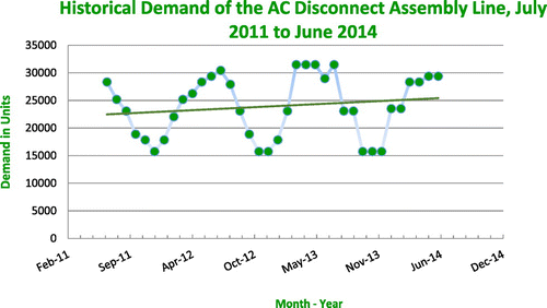
Note. The demand during this period shows a regular pattern with seasonality and a slight upward trend.
We considered a slope and intersection values of 84.459 and 22,383 for the linear regression and the double exponential smoothing methods. To enable what-if analysis, we optimized the smoothing parameters α = 0.1 and β = 0.1 for the double exponential smoothing method only. The what-if analysis consists of adjusting the values of α and β in the equation to evaluate how those adjustments affect the outcome. In this case, the parameters were selected to reduce the forecast error.
In Figure 5, we present a comparison of the monthly historical demand and the forecast obtained using the simple linear regression method with a mean absolute percentage error (MAPE) of 22%. This error directly impacts the capacity at the work centers and causes frequent adjustments in the required numbers of operations personnel.
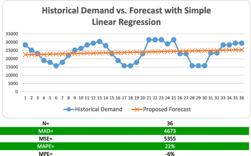
Figure 6 shows the comparison of the monthly historical demand and the forecast obtained using the double exponential smoothing method with a MAPE of 23%. As presented, there is no improvement.
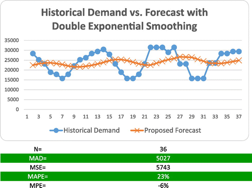
As part of the forecast evaluation, we performed analyses of forecast errors, such as the MAPE, median absolute deviation (MAD), mean squared error (MSE), and mean percentage error (MPE), as Hanke and Wichern (2009) discuss.
Because the errors did not decrease, we decided to adjust the average demand in our analyses from monthly to quarterly. We considered the average demand from July 2011 to June 2012 as the initial base and zero as the initial trend with optimized smoothing parameters of α = 0.1 and β = 0.1, and seasonal factors of 1.09, 0.70, 0.99, and 1.22, respectively, for each quarter using the double exponential smoothing method. With this adjustment, the errors decreased from 23% to 4%.
In contrast, the errors using the simple linear regression method decreased only from 22% to 20%. See Figures 7 and 8.
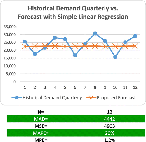
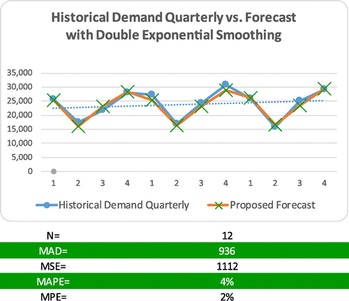
Figure 7 shows the quarterly historical demand versus the forecast obtained by the simple linear regression method with a MAPE of 20%. Although we adjusted the demand, the forecast showed no significant improvement.
Figure 8 shows the quarterly historical demand versus the forecast obtained by the double exponential smoothing method with a MAPE of 4%. We can observe that the demand has a predictable behavior. Thus, we conclude that the double exponential smoothing method is more efficient than simple linear regression.
Phase 2
Once we obtained the forecast of the double exponential smoothing method, we integrated it into the aggregate planning of the AC disconnect assembly line to determine the best strategies to use in accordance with STP’s requirements.
Commonly, the use of single or mixed strategies works well when demand forecasting has a certain degree of smoothing with minimal error coefficients. In this case study, the mixed strategies are not applicable because Schneider manufactures safety products and cannot outsource partial or total manufacturing to an external supplier. Hence, we used chase and level strategies because, according to Chase et al. (2000) and Heizer and Render (2004), they produce good results when used for aggregate planning.
With the chase strategy, only enough goods are produced to meet (or exactly match) the demand for goods. This strategy has the advantage of keeping inventories low, which reduces inventory carrying costs. This frees up cash that can be used for other needs. A disadvantage of this strategy is that it requires the constant hiring, training, and firing of personnel with changes in the demand (Sule 2008).
Conversely, with the level strategy, the company continuously produces goods equal to the average demand. The same quantities of goods are scheduled consistently through a specific period; consequently, the number of personnel needed is constant (Sule 2008).
STP has used the chase strategy for many years; therefore, our evaluation involved identifying whether changing to a level strategy could increase profit and reduce operating costs.
Some items we considered in evaluating strategies were the costs of materials for manufacturing; holding inventory costs; the marginal costs of stockouts; costs of personnel hiring, training, and firing; salaries; working hours; initial inventory costs; productivity; sale prices; and initial level of the workforce.
When we tested a six-month forecast, from January 2014 to June of 2014, we achieved the following results using the chase strategy: operating cost of $1.03 million, income of $2.11 million, and profit of $1.07 million. In contrast, using the level strategy, we achieved these results: operating cost of $1.15 million, income of $2.11 million, and profit of approximately $962,350. Using the chase strategy, the operating cost is lower and profit is higher because labor is less expensive. Therefore, we did not change the strategy. Table 1 shows a comparison of plans with different strategies using the forecasted demand from January 2014 to June of 2014.
|

Table 1. A Comparison of Aggregate Planning from January 2014 to June 2014 Using the Chase and Level Strategies
| Forecast January–June 2014 | ||
|---|---|---|
| Chase strategy | Level strategy | |
| Operating cost (USD) | $1,032,908.80 | $1,149,050.07 |
| Income (USD) | $2,111,394.60 | $2,111,394.60 |
| Profit (USD) | $1,078,485.80 | $962,344.53 |
Note. A comparison of aggregate planning from January 2014 to June 2014 using the chase and level strategies led us to conclude that the chase strategy is superior to the level strategy for STP.
In the same way, we evaluated both strategies in comparison with the forecast for the period from January 2015 to June of 2015. Similarly, the chase strategy worked better for the company. Table 2 shows the comparison of plans with different strategies using the forecasted demand from January 2015 to June 2015.
|
Table 2. A Comparison of Aggregate Planning from January 2015 to June 2015 Using the Chase and Level Strategies
| Forecast January–June 2015 | ||
|---|---|---|
| Chase strategy | Level strategy | |
| Operating cost (USD) | $906,606.23 | $1,004,800.96 |
| Income (USD) | $1,874,301.12 | $1,874,301.12 |
| Profit (USD) | $967,694.89 | $869,500.16 |
Note. A comparison of aggregate planning from January 2015 to June 2015 using the chase and level strategies also led us to conclude that the chase strategy is superior to the level strategy for STP.
Our conclusion was that STP should make no strategy changes.
Phase 3
Consequently, the batch sizes of cabinets had to be readjusted for daily manufacturing to establish the number of each component to be manufactured each day and to find the point of “economic balance” between long production runs and inventory costs.
We used the forecast period from January 2015 to June of 2015 as the base to recalculate the batches. During this period, the forecast did not change significantly, and the average quarterly demand was 24,048 finished products.
We used the EOQ model to calculate the optimum-level batch of assembled cabinets for supplying the AC disconnect line. We selected this model because of the coefficient of variability (CV) of the quarterly historical demand, which we computed as 19%. Because the CV was less than 20%, we determined the variability of the demand to be low; thus, we used a deterministic inventory model. The EOQ model was considered to minimize the ordering and to hold logistic costs associated with the inventory (Schniederjans and Cao 2001); see Appendix A.
We estimated the optimal batch size to be 514 pieces. After making a sensitivity analysis, we decided to establish the batch size at 500 pieces for each type of stamped part because one of each stamped part is used in the assembled cabinet; that is, the assembled cabinet includes one of each component.
Based on the aggregate planning for this project, for which we used the chase strategy, we estimated the average monthly requirement to be 24,048 pieces for the final assembly line. As a result, by considering an average of 20 workdays per month, we estimated the daily consumption of each manufactured component to be 1,202 pieces. Therefore, three orders of 500 pieces of each component must be manufactured each day, so 1,202 pieces of each component will be used, and the remaining 298 pieces of each component, equivalent to 4.7%, can be used as safety stock; this amount of safety stock can easily cover the forecast error.
In Tables 3, 4, and 5, we present comparisons of previous and current batch productions.
|
Table 3. Daily Production Quantities for Each Component Before the Recalculation of the EOQ
| Components | Previous EOQ | Previous daily production |
|---|---|---|
| F–S2 | 1,344 | 8,064 |
| SON1 | 2,000 | 12,000 |
| SON2 | 1,000 | 8,000 |
| F–S1 | 1,512 | 6,048 |
Note. Each component has a different batch size and each was manufactured in quantities of six, six, eight, and four times its EOQ, respectively.
|
Table 4. Daily Production Quantities After Recalculation of the EOQ
| Components | Current EOQ | Current daily production |
|---|---|---|
| F–S2 | 500 | 1,500 |
| SON1 | 500 | 1,500 |
| SON2 | 500 | 1,500 |
| F–S1 | 500 | 1,500 |
Note. Each component has the same batch size of 500 pieces and each is manufactured in quantities of three times its EOQ.
|
Table 5. Daily Reduction of Manufactured Components
| Components | Batch reduction in pieces |
|---|---|
| F–S2 | 6,564 |
| SON1 | 10,500 |
| SON2 | 6,500 |
| F–S1 | 4,548 |
Note. The reduction approximates 28,112 components.
Finally, we analyzed the records showing manufacturing, tool-change, and adjustment times, which we determined to take an average of 39 minutes and to be the cause of long production runs. The implementation of the SMED methodology and the creation of a pit-stop team significantly reduced the tool-change time from approximately 39 minutes to 9 minutes because of modifications to the dies. It also reduced delivery times, eliminated excessive storage costs, and increased the production output.
STP invested $7,500 in the SMED implementation. This budget was used to buy spare parts and the tools required to ensure that the machine setup times would be less than 10 minutes. By reducing the batch size and setups times, the number of KB cards was also reduced. As we mention above, these cards provide important information about the quantities of the various components to be supplied and produced.
To establish the correct number of KB cards in the system for each product, we used the common KB calculation equation (Ramnath et al. 2009); see Appendix B.
Table 6 shows savings we obtained. Previously, there were 49 KB cards, equivalent to a three-day supply of material to the stamping operation. These quantities had to be stored in 49 physical spaces of 1.3 m3 each. The holding inventory cost was $21,851.63. After the implementation of continuous flow, the improvements were significant; the lead time for the stamping operation was reduced from three days to two days, and the number of KB cards decreased from 49 to 24. This also eliminated the need for storage and reduced the holding costs and the inventory levels by 78% and 77.65%, respectively.
|
Table 6. We Obtained Significant Savings by Recalculating the KB Cards
| Before the implementation | |
|---|---|
| Inventory amount | $21,851.63 |
| Number of locations in warehouse | 49 |
| Lead time: stamped parts | 3 |
| Kanban cards in system | 49 |
| After the implementation | |
| Inventory amount | $4,883.62 |
| Number of locations in warehouse | 0 |
| Lead time: stamped parts | 2 |
| Kanban cards, recalculation | 24 |
| Total savings | |
| Inventory amount | $16,968.01 |
| % inventory reduction | 77.65 |
| # locations in warehouse eliminated | 49 |
| Lead time (reduction in days) | 1 |
| Kanban card reduction | 25 |
This decision to recalculate the number of KB cards helped to eliminate the inventory of components and subassemblies manufactured in-house, which were used in the finished product. This allowed STP to release space in the warehouses and consequently reduce excessive transportation of materials.
As Figure 9 shows, although each component is processed in the same sequence as previously, it is now processed and sent directly to the next operation, thus avoiding the necessity for storage in a warehouse.
This flow of components and subassemblies is achieved by synchronizing the demand-planning, materials-planning, and manufacturing processes and warehouse operations. First, the F–S1 and F–S2 components are stamped and painted; at the same time, the components SON1 and SON2 are stamped, welded, and painted. And finally, all of these components are assembled to produce a cabinet, which will be sent again to the painting operation to fine-tune the painting process. When the cabinets have dried, they are sent to the final assembly line.
Eliminating the unnecessary transportation to and from the warehouse generated personnel and energy (i.e., vehicle) savings of up to $26,000 per semester (in our case, the first half of the year).
In addition, in the short term, the service level increased to the desired target level. Since the implementation in October 2014 until September 2016, the target service level of 98% was achieved. The service level did not reach the target in only three months during this period—April 2015 (97.5%), May 2015 (95.5%), and February 2016 (60%). This happened because external suppliers of certain subassemblies encountered problems in delivering to the plant. This situation must be analyzed; although the supply contract specifies penalties for nondelivery, these stockouts produce stress in the line. Figure 10 presents a comparison of the service level before and after implementation of the methodology in the line. Before the implementation, the service level was below the target or objective of 98% in 8 of 24 months. In contrast, after the implementation (and because of external situations), the service level was below the objective in only 3 of 24 months. As presented, therefore, the implementation provided service-level improvements.
In Table 7, we summarize the results we obtained. Although the total investment was made once, the savings are ongoing. After 24 months, these savings exceeded $1 million. We calculate this by totaling the inventory costs, which are the costs for each component, the movement costs that result from reducing the use of resources (e.g., forklift, fuel, employees), and operational costs using the chase strategy.
|
Table 7. Based on the Investment that STP Made, Savings and Improvements Obtained Are Substantial
| Savings | |
|---|---|
| Inventory amount | $407,232.24 |
| Movement cost reduction | $105,724.96 |
| Operational cost using chase strategy | $505,210.28 |
| Total savings | $1,018,167.48 |
| Improvements | |
| % inventory reduction | 77 |
| Number of warehouse locations | 49 |
| Lead-time reduction for stamped parts (in days) | 1 |
| Kanban card reduction | 25 |
| Investments | |
| SMED tools | $7,500.00 |
| JIT containers | $4,500.00 |
| Training | $800.00 |
| Total investment | $12,800.00 |
Project Impact, Lessons Learned, and Concluding Remarks
We achieved a successful implementation of continuous flow and enhanced four of the company’s key processes in the areas of the demand-planning, materials-planning, and manufacturing processes and warehouse operations. Information sharing improved a series of logistics activities that are critical for ensuring the delivery of the finished product to the end customer on schedule and that managers in each area carry out.
STP became the first Schneider plant to implement this practice, which the Schneider production system (SPS) internal audit system now requires. Communication between the various departments increased, thus improving efficiencies in day-to-day processes.
Since the implementation of continuous flow in October 2014, stoppages or delays on the assembly line have been eliminated, and savings of approximately $3.5 have been generated. STP’s investment of $12,800 represented only 1.25% of the savings estimated until September 2016. STP can now handle the seasonal rise in demand and reach its target service level.
The storage configuration of warehousing for components and subassemblies was eliminated from the ERP system. This allowed the release of 49 storage spaces. In addition, monthly savings of approximately $4,400 were obtained by eliminating the unnecessary transportation of components and subassemblies.
Using the SMED methodology, modifications of the dies reduced the setup time from 39 minutes to 9 minutes in the tool-change operation. This represents a time savings of 77%. The creation of a pit-stop team was an important achievement because STP was the first plant to implement this practice.
As suggested, the KB cards must be recalculated for all the stamped parts that comprise the various cabinet styles.
With the implementation of lean tools, the work-in-process (WIP) inventory and subassemblies, cycle times, and delays between processes were reduced.
An additional benefit to Schneider Electric was that it was able to successfully replicate this methodology in similar lines at its plants in North America. The methodology’s adoption as a good practice will support strategic decisions. In 2014, STP was awarded first place in an SPS international audit (Manufactura 2014, Schneider Electric 2014).
As part of future work, this methodology will be implemented in STP’s eight remaining production lines. However, this may require the use of other complex tools because of the greater mix of finished products.
This research was developed in the master's program “Logistics and Supply Chain Management” at Universidad Popular Autónoma del Estado de Puebla (UPAEP), awarded with standard of excellence by Programa Nacional de Posgrados de Calidad, and supported with resources granted by the National Science and Technology Council (Consejo Nacional de Ciencia y Tecnología) – CONACyT. Scholarship holder number: 287098.
Appendix A
The EOQ model is as follows:
where D = demand, S = ordering cost, H = holding cost, and Q = economic order quantity.
Appendix B
The KB calculation equation is as follows:
where D = demand, Lt = lead time, SS = safety stock, and EOQ = economic order quantity.
References
- (2013) Improvement of setup time and production output with the use of single minute exchange of die principles (SMED). Internat. J. Engrg. Res. 2(4):274–277.Google Scholar
- (2013) Practice summary: Enhancing forecasting and capacity planning capabilities in a telecommunications company. Interfaces 43(4):385–387.Link, Google Scholar
- (2001) Selecting methods: Selecting forecasting methods. Armstrong JS, ed. Principles of Forecasting: A Handbook for Researchers and Practitioners (Kluwer Academic Publishers, Norwell, MA), 365–386.Crossref, Google Scholar
- (2004) Business Logistics: Supply Chain Management, 5th ed. (Pearson Education, Naucalpan de Juárez, Mexico).Google Scholar
- (2011) Single minute exchange of die: A case study implementation. J. Tech. Management Innovation 6(1):129–140.Crossref, Google Scholar
- (2009) An integrated outbound logistics model for Frito-Lay: Coordinating aggregate-level production and distribution decisions. Interfaces 39(5):460–475.Link, Google Scholar
- (2000) Management and Administration of Production and Operations, 7th ed. (McGraw-Hill Irving, Barcelona, Spain).Google Scholar
- (2000) Comparison among three pull control policies: Kanban, base stock, and generalized kanban. Ann. Oper. Res. 93(1–4):41–69.Crossref, Google Scholar
- (1994) Sistemas de programación y planeación agregada. Administración de la Producción y las Operaciones: Conceptos, Modelos y Funcionamiento, 4th ed. (Prentice-Hall Hispanoamericana, Mexico), 409–441.Google Scholar
- (2009) ASP, the art and science of practice: Tales from the front: Case studies indicate the potential pitfalls of misapplication of lean improvement programs. Interfaces 39(6):540–548.Link, Google Scholar
- (2004) Do we think we make better forecasts than in the past? A survey of academics. Interfaces 34(6):466–468.Link, Google Scholar
- (2009) Business Forecasting, 9th ed. (Pearson Education, Harlow, UK).Google Scholar
- (2004) Aggregate planning. Principles of Operations Management, 5th ed. (Pearson Education, Naucalpan de Juárez, Mexico), 487–518.Google Scholar
- (2014) Supply chain scenario modeler: A holistic executive decision support solution. Interfaces 44(1):85–104.Link, Google Scholar
- (2012) Os efeitos do just-in-time sobre o desempenho financeiro das empresas. Revista de Gestão, Finanças e Contabilidade 2(2):35–46.Google Scholar
- (2015) People skills: Building analytics decision models that managers use—A change management perspective. Interfaces 45(4):363–364.Link, Google Scholar
- (2009) Correcting heterogeneous and biased forecast error at Intel for supply chain optimization. Interfaces 39(5):415–427.Link, Google Scholar
- Manufactura (2014) 4 historias de éxito LEAN. Manufactura, Información estratégica para la Industria (October 2014), http://dimensionx.com.mx/MagazineDigitalDesktop/Manufactura/octubre2014/.Google Scholar
- (2005) Kanban implementation at a tire manufacturing plant: A case study. Internat. J. Manufacturing Res. 16(5):488–499.Google Scholar
- (2008) Spreadsheet decision-support tools: Lessons learned at Hewlett-Packard. Interfaces 38(4):300–310.Link, Google Scholar
- (2009) Inventory optimization using kanban system: A case study. IUP J. Bus. Strategy 6(2):56–68.Google Scholar
- (2013) The use of SMED to eliminate small stops in a manufacturing firm. J. Manufacturing Tech. Management 24(5):792–807.Crossref, Google Scholar
Schneider Electric (2014) Success stories: Tlaxcala plant is positioned in the first place worldwide in the annual audit SPS Schneider production system. Open Up Schneider Electric. 31.Google Scholar- (2001) An alternative analysis of inventory costs of JIT and EOQ purchasing. Internat. J. Phys. Distribution Logist. Management 31(2):109–123.Crossref, Google Scholar
- (2008) Production Planning and Industrial Scheduling: Examples, Case Studies, and Applications, 2nd ed. (CRC Press, Boca Raton, FL).Google Scholar
- (2000) Innovations in competitive manufacturing: From JIT to e-business. Swamidass PM, ed. Innovations in Competitive Manufacturing (Springer Science+Business Media, New York), 3–13.Google Scholar
- (2010) General Electric uses an integrated framework for product costing, demand forecasting, and capacity planning of new photovoltaic technology products. Interfaces 40(5):353–367.Link, Google Scholar
- (2000) The role of just-in-time in supply chain management. Internat. J. Logist. Management 11(1):89–98.Crossref, Google Scholar
- (2006) Forecasting and sales & operations planning synergy in action. J. Bus. Forecasting 25(1):16–36.Google Scholar
- (2007) A web-based Kanban system for job dispatching, tracking, and performance monitoring. Internat. J. Adv. Manufacturing Tech. 38(9/10):995–1005.Google Scholar
Verification Letter
Mr. Horacio Galicia Peréz, Tlaxcala Plant Operations Manager, Schneider Electric, North America Operating Division, Vía Corta Sta Ana-Puebla, Tlaxcala C.P. 90860, Mexico, writes:
“I am writing to you to certify that the student/employee Rodolfo Rodríguez-Méndez, along with the areas of Demand Planning, Manufacturing, Production and Warehouse, has succeeded in concluding the project ‘Implementation of Continuous Flow in the Cabinet Process at the Schneider Electric Plant in Tlaxcala, Mexico,’ which was developed during the period from May 26th to November 28th, 2014.
“This project was implemented after being reviewed and approved by the Managers [of the] corresponding area; of course it has added great value to our operation and the positive impact of this is specifically reflected in the areas of Production and Inventory, getting substantial savings by 77% in the inventory reduction equivalent to $16.9K, and also managed to streamline our processes specifically in the presses area with the application of the SMED methodology to reduce the setup time in all parts involved from 39 minutes to 9.5 minutes. The Warehouse area also was benefited with 49 free spaces that we will not use more in the future. We are expecting to get savings in average by $126K in the first semester of 2015 due to the usage of the aggregate planning with the methodology of the ‘demand chase’ proposed in this project together with the demand smoothing.
“This letter certifies that the project ‘Implementation of Continuous Flow in the Cabinet Process at the Schneider Electric Plant in Tlaxcala, Mexico‘ has completed all required tasks in the project plan and all phases of the Enterprise Methodology. All user requirements have been met, all issues have been resolved, and all required deliverables have been approved.
“[Although] the usage of general information is authorized,…use of detailed information on the processes where the project was developed [is not]. The use of engineering drawings is not authorized. This information must be used only for educational purposes, both in this thesis project developed by Rodolfo Rodríguez-Méndez [and] the indexed article developed.
“Schneider Electric gives thanks in advance to Logistics and Supply Chain Management Program at UPAEP University, for the direction you give to their students to develop these kinds of practices in which learning is evaluated in the field.”
Diana Sánchez-Partida is currently a professor-researcher in logistics and supply chain management at Universidad Popular Autonoma del Estado de Puebla (UPAEP) in Mexico. She is a member of the National Research System (Level 1). Her areas of interest are logistics, design, and optimization of the supply chain, and humanitarian logistics. She has participated in applied projects such as timetabling for schools, levels of inventories, and production planning.
Rodolfo Rodríguez-Méndez has a master’s degree in logistics and supply chain management. He is currently a systems, applications, and products (SAP) plant master data analyst working for Schneider Electric in Tlaxcala, Mexico. He provided support regarding logistics data management to Schneider Electric's Mexico City and Costa Rica plants. He is interested in the areas related to SAP logistics data management, like distribution execution and supplier relationship management.
José Luis Martinez-Flores is a researcher and academic director in the Department of Logistics and Supply Chain Management at UPAEP. His objectives are research and consultancy. He designs and executes the models for the planning and optimization problems in the field of logistics through the use of information technologies for the length of the supply chain.
Santiago-OmarCaballero-Morales is a professor and researcher in the Department of Logistics and Supply Chain Management at UPAEP. In 2009, he received a PhD in computer science from the University of East Anglia in the United Kingdom. Since 2011, he has been a member of the National Council of Researchers in Mexico. His research interests are operations research, combinatorial optimization, pattern recognition, and human-robot interaction.

