


Fast Selection from Multiple Treatments: A Sequential Method for Principled Digital Experimentation
Abstract
In the current era of digital business, firms continuously experiment to enhance the online experience of individuals visiting their websites and platforms. The possible changes range from minor tweaks to large product or user experience updates, which are tested before full rollout to estimate performance and minimize unintended negative outcomes. Because of the clear benefits of digital experimentation, increases in the number of experiments have strained the resources of online participants/customers. In tension with this scarcity, many digital experiments are not carefully powered for their objectives, leading to either oversampling that wastes resources or undersampling that weakens inference. These issues warrant methods that can help experimenters balance power and efficient resource use—that is, to sample enough for proper power without oversampling. To address this issue, we propose a sequentially sampled hypothesis testing method for selecting the best treatment among multiple alternatives for experimenter-specified levels of statistical power and false positive rate. Critically, the method not only samples for no more than the necessary level of statistical power; it also has low sample size variance relative to other methods, meaning that the resulting sample size is a precise estimate of the required sample size and low bias in the treatment effect estimates, reducing a common problem for adaptive sampling methods. We also demonstrate our method on a data set from a real multiarmed online experiment, which demonstrates the method’s efficacy in a realistic scenario. Our method can be implemented in an experimentation pipeline, facilitated with an R package we provide.
History: Gautam Pant, Senior Editor; Yixin Lu, Associate Editor.
Supplemental Material: The online appendix is available at https://doi.org/10.1287/isre.2024.1537.
1. Introduction
Today, many large digital firms continuously experiment to keep up with competitors and adapt to changes in technology and the mercurial nature of consumer behavior and preference. Firms that use digital experimentation seek to establish causal attribution and risk mitigation for novel product or platform changes (Bojinov and Gupta 2022). Further, empirical evidence has demonstrated performance benefits to technologically advanced firms that adopt thorough experimentation approaches to decision making (e.g., Koning et al. 2022).
The benefits of consistent experimentation are substantial, but participants are not an infinite resource. Even on large platforms with many users, the large number of simultaneous experiments and typically small effect sizes—which require considerable sample sizes to be detected reliably—can put a strain on participant resources. Scarcity of participants compels companies to use strategies to get the most out of a limited resource. One approach is to apply many treatments to each participant simultaneously, typically via an orthogonal test plane. Abbasi et al. (2025) demonstrate the unintended consequences of this approach, namely, that the unaccounted-for interaction effects can bias marginal treatment effect estimates, unbeknownst to product managers or scientific partners. One way to sidestep this issue is to assign individuals to only one treatment when tests for more substantial product/platform changes are being made (and minimal bias matters most), but this naturally worsens scarcity.
Alternatively, adaptive procedures can be used to minimize sampling. For these methods, the sample size assigned to a given treatment or policy change is determined as the sampling and parameter estimation unfold, usually with the objective of sampling less from low-performing treatments or to stop sampling as soon as there is sufficient evidence to make a decision. However, adaptivity has been shown to bias treatment effect estimates (Nie et al. 2018), and the bias generally worsens the more adaptive a method is. Estimation bias hinders post hoc studies such as heterogeneous treatment effect analysis, which has been noted as one of the key advantages of online experiments (Karahanna et al. 2018). Reliable follow-up studies then require new samples, worsening scarcity.
Scarcity is in tension with the problem of powering studies sufficiently. Kohavi et al. (2022) reveal that power analysis for hypothesis testing is poorly understood and often ineptly applied in practice in digital experimentation, even by A/B testing consulting firms. This often results in greatly underpowered studies, increasing the uncertainty in decision making and rendering the expended resources effectively useless. Powering analysis is also dependent on knowledge of generally unknown population parameters, such as the variance of the outcome (Cohen 1988), heightening the uncertainty of the test results.
To balance the opposing challenges of scarcity and power for accurate decision making, we propose that firms should use methods that reliably identify the smallest amount of experimentation necessary for accurate decision making while biasing the samples minimally and enabling valuable post hoc analysis. This article proposes such an approach in the setting of comparison and selection among multiple treatments against an incumbent treatment (business as usual) or baseline performance requirement. Our method frames this problem in the null-hypothesis significance testing (NHST) framework, allowing the experimenter to separately specify the error rate of rejecting the standard when there is in fact no better alternative (Type I error) and the error rate of failing to select an existing better alternative (Type II error), unlike most methods of selection and comparison with a standard, which generally fix a single probability of correct selection for the standard and alternatives. Our method then tailors a sequential sampling procedure to accurately and precisely estimate the ideal sample size that meets exactly the desired error rates given the experimenter’s definition of sufficient improvement to implement a change. This aligns statistical power and practical significance as defined by the experimenter (i.e., the minimum effect size that would warrant policy change). Critically, the sequential estimation of the nuisance parameters facilitates a precise estimate of the ideal sample size for the task, meaning our method over- or undersamples very little relative to existing similar methods.
Additionally, whereas this method samples adaptively, it uses sample mean information sparingly. Consequently, the treatment effect estimates are substantially less biased in comparison with many other competitive methods. This better enables post hoc analysis of the treatment effects, such as the examination of heterogeneous treatment effects.
In summary, our method has the following desirable and practical properties, making it uniquely suited for the current state of digital experimentation:
The method samples minimally, producing results close to the exact power and size specified, where many methods far oversample and overdeliver on the correct selection rate.
The necessary sample size is precisely estimated, resulting in a far narrower upper tail in the sample size distribution in comparison with other methods.
The method makes minimal distributional assumptions on the outcome.
The method biases treatment effect estimates minimally relative to other methods.
No hyperparameter tuning: experimenters only supply parameters following from their problem and preferences; other design parameters are optimized by a procedure we provide.
The organization of this article is as follows. In Section 2, we discuss state-of-the-art methods in digital experimentation, especially for best treatment selection. In Section 3, we formalize the problem and propose the sequential best treatment selection method. Section 4 presents a novel optimization approach that determines the derived design parameters for our method, tailoring the sequential method to the experimenter’s preferences on error rates and practical significance thresholds. Section 5 presents the results of simulation studies demonstrating its performance characteristics and comparisons with existing methods on several criteria, and includes an analysis of data from a real online experiment. In Section 6, we give concluding remarks.
2. Relevant Literature
Digital experimentation methods have become increasingly relevant to the management and information systems (IS) literature. These developments generally approach managerial problems with interesting statistical solutions. Some recent examples include (a) handling interference and heterogeneous effects with switchback experiments (Bojinov et al. 2023), (b) optimizing the design of staggered rollouts for estimating both short-term and long-term treatment effects (Xiong et al. 2024), and (c) always-valid inference methods that protect Type I error rates from “A/B peeking” (data-dependent test stopping) (Johari et al. 2021).
This paper proposes a method in a similar vein to statistical methods for management problems. We develop a novel application of NHST in an algorithmic approach for selecting the best of many treatment arms with comparisons to a standard. In the remainder of this section, we review NHST’s use in digital experimentation and survey existing selection methods, to which we will compare our method.
2.1. Null-Hypothesis Significance Testing in Digital Experiments
In contrast with advances in digital experimentation methods, much of the experimentation in practice is statistically or practically naive, in part because of the sometimes-onerous implementation of theoretically powerful methods. This appears to be especially so for sample size planning for statistical goals (Kohavi et al. 2022). Often, power is not directly considered, and a rule of thumb is used, such as setting data collection to conclude after a fixed period of time, such as two weeks (Kohavi et al. 2013). Alternatively, a fixed n is determined in advance using power analysis, which presupposes some (typically unknown) information about the population. Both approaches regularly result in studies with unnecessarily high power or unacceptably low power with respect to the managerial goals of the evaluation (see Maxwell et al. (2008) for a review of sample size planning methods). Kohavi et al. (2022) emphasize the prevalence of underpowered studies and demonstrate the unreliability of the results produced. Thus, they recommend that experimenters use approaches that are high powered for the typically small effects seen in online settings.
A secondary problem in digital NHST practice identified in the IS and operations literatures is Type I error inflation because of “peeking” or data-dependent test stopping (Johari et al. 2017). The evidence of this kind of error inflation in the field is mixed, with some evidence that it is fairly prevalent (Berman et al. 2018) and some evidence that it is less common in business than in academic research (Miller and Hosanagar 2025). To the degree that this is a real issue, studies that are planned for sufficient power can address it by controlling Type I errors.
Despite its wide use in the field, Feit and Berman (2019) contend that NHST is not ideal for the digital experimentation setting and that less robust testing is more cost-effective. They cite the relatively low consequence of Type I errors, NHST’s high sample size requirement, and the lack of a clear decision when the null is not rejected. Whereas their alternative approach seems quite suitable for marginal changes and tweaks, we believe that many online experimentation settings do justify the NHST framework, especially in cases where more substantial changes are proposed (e.g., new recommender algorithms, large user interface (UI) changes) or there are high-stakes outcomes.
Through qualitative analysis, Koning et al. (2022) discover that firms that successfully implement digital experimentation test both incremental adjustments as well as larger product and website changes. When testing these more substantial changes, Type I errors are not so low cost and can, in fact, result in significant losses or missed opportunities if the implementation of a product has negative effects that are not detected in testing. Additionally, when an experiment is appropriately powered, it is clearer that adhering to the incumbent product or user experience is a reasonable decision when the null is not rejected by the test, so the decision under the null is clear.
2.1.1. Sample Size Planning and Sequential Estimation for NHST.
As Kohavi et al. (2022) emphasize, well-powered studies are key to accurate decision making. Sample size planning is a central part of this process, in which experimenters determine the necessary sample size required to make accurate decisions, conditional on the desired power, Type I error, population effect size, and variance (or a variance-standardized effect size of interest; see Cohen 1988). Nuisance parameters like the population outcome variances must be specified a priori to preplan the sample size of a study to achieve a desired level of power at a given Type I error rate for a given effect size. Population parameters are often difficult to provide because the population parameters are generally unknown. They are often estimated with a small pilot sample, which will tend to render high-variance estimates. Nelson and Goldsman (2001) and Rollin and Chen (2005) exemplify this approach in the best treatment selection literature.
Sequential analysis circumvents the difficulty of presupposing (or estimating with a small pilot sample) unknowable population values by determining sample size a posteriori instead of a priori: samples are drawn successively until a prespecified condition, called the stopping rule, is satisfied. The procedure can then conclude dynamically (in a data-dependent fashion) while controlling desirable statistical properties, and the stopping rule can use all samples up to the stopping point to estimate nuisance parameters such as the variance, which has benefits such as generating precise estimates of the ideal sample size. Notable examples from selection and other statistical domains include Kim (2005), Bandyopadhyay and Biswas (2015), and Kelley et al. (2018).
2.2. Treatment Selection Methods
The problem of selecting the best from several alternatives or arms is addressed by two related but distinct literatures: ranking and selection (R&S) and pure-exploration multiarmed bandit (MAB) algorithms. Although these two domains make different statistical assumptions about the alternatives and seek somewhat different theoretical results, both domains seek to efficiently select the best treatment at a user-specified probability of correct selection. Here, we discuss existing methods from both domains and contrast them with our approach.
A key element shared by many of these methods is the indifference margin. Practically, distinguishing between two arbitrarily close treatments can require an enormous amount of sampling for little gain. Accordingly, the indifference margin is a minimal distance worth detecting, akin to the effect size of interest used to plan sample size in power analysis. If the difference between the mean of the second-best treatment and the mean of the best treatment is less than the indifference margin, then the second-best treatment may be selected at a higher rate than requested because it is deemed “close enough” to the best. In R&S, this margin is generally referred to as the indifference-zone (IZ), whereas MAB algorithms commonly denote it with (Mannor and Tsitsiklis 2004, Even-Dar et al. 2006).
Without specifying a minimal effect difference worth detecting, a selection algorithm’s goal will be to distinguish between arbitrarily close treatments. Few R&S methods take this approach (see Fan et al. (2016) and related work for a notable exception), whereas many algorithms in the MAB literature do. We believe that this objective is generally not relevant in the digital experimentation setting because the cost of distinguishing between arms with arbitrarily small differences can be extremely high and the returns are as small as the differences.
2.2.1. Ranking and Selection Literature.
Our approach is closely related to a family of R&S algorithms termed “comparisons with a standard,” where a set of alternative proposed treatments is sampled to determine whether any are superior to a standard or existing treatment. For example, Nelson and Goldsman (2001) studied this problem and proposed a two-stage method to estimate the sample size necessary to distinguish the best from a standard and the inferior treatments, akin to fixed sample size planning for a selection task. This two-step approach can be improved with sequential sampling, where the ideal sample size is estimated as samples sequentially arrive, using far more information to precisely determine the total number of samples needed.
Kim (2005) developed a sequential procedure for selecting the best treatment among alternatives and a standard. Her approach uses the initial sample size to estimate the variances of each arm and sequentially samples from each arm, adaptively dropping out apparently inferior treatments. Sequential sampling approaches to R&S can update estimates of nuisance parameters (such as outcome variances) as they go, allowing stopping decisions to be based on high-precision estimates. This will generally reduce the variation in stopping, reducing drastic over- or undersampling because of noisy nuisance parameter estimates. However, this approach requires additional theoretical care. Both the KN++ algorithm proposed by Kim and Nelson (2006) and our method presented in this paper update sample variances sequentially, allowing for more controlled, lower-variance stopping.
We note that the aforementioned R&S algorithms, as well as ours, are oriented in the frequentist perspective to statistical inference. Related work addresses the problem in a Bayesian framework, which can be advantageous, depending on the context and goals (see, for example, Chick and Frazier 2012, Xie and Frazier 2013). Bayesian approaches tend to optimize the sampling and decision process for the expected value across a distribution of possible realities, whereas the frequentist approach tends to optimize for a worst case (typically specified by the IZ). We believe that specifying the minimum worthwhile difference to detect is more intuitive and easier to apply in the context of digital experimentation for managers than specifying a multidimensional prior distribution.
2.2.2. Multiarmed Bandit Literature.
The selection problem this paper addresses is similar to multiarmed bandit problems (Schwartz et al. 2017, Hu et al. 2022). A subclass of MAB problems geared toward pure exploration, often called best arm identification (BAI) methods, comprises methods specifically designed for the selection of the best treatment alternative and is thus most similar to our setting. Especially similar to our work are the “probably approximately correct” (PAC) BAI algorithms that make guarantees of finding an arm within an indifference margin of the true best arm at a specified error rate.
Among others, Even-Dar et al. (2002) and Mannor and Tsitsiklis (2004) pioneered the treatment of this problem in the MAB literature, providing theoretical upper and lower bounds, respectively, on the sample complexity required to identify a near-best arm, with Even-Dar et al. (2006) providing an algorithm that matches the lower bound up to constants. More recent work has further lowered the theoretical sample complexity and developed more efficient algorithms. Two foremost examples are the lil’UCB algorithm (Jamieson et al. 2014) and the Track-and-Stop strategy (Garivier and Kaufmann 2016).
MAB algorithms generally assume Gaussian (or sub-Gaussian or exponential-family) arms with known nuisance parameter values such as arm outcome variance (e.g., Jamieson et al. 2014, Garivier and Kaufmann 2016, Barrier et al. 2022) or else make minimal assumptions except a known bound on the support (e.g., Even-Dar et al. 2006, Karnin et al. 2013), enabling the use of Hoeffding inequalities in the construction of the correct selection guarantees. In contrast, many R&S algorithms make a distributional assumption (e.g., Gaussian) or rely on asymptotics via the central limit theorem (CLT), and many estimate unknown nuisance parameters such as the variance as part of the procedure.
MAB BAI analysis is generally concerned with the lower and upper bounds on the sample complexity, and an optimal algorithm in this setting is one that scales proportionally to the lower bound with respect to the key problem parameters (such as rate of correct selection and indifference margin) “up to constants,” regardless of the size of those constants. This often results in algorithms that are quite conservative in terms of their success rate guarantees, gathering far more samples than their R&S counterparts. To demonstrate this, we include lil’UCB in our main simulation comparisons (Section 5.2) and discuss the sampling behavior of Even-Dar et al. (2006) and Karnin et al. (2013) in our studies with binary outcomes (Section C.3.1 in the Online Appendix and Section 5.4). Although R&S algorithms are, in some dimensions, more practical than MAB approaches, the MAB literature provides strong theoretical analysis of the selection problem, which is invaluable for the field.
3. A Sequential Method for Selecting the Best Treatment
Our procedure builds on a family of two-phase selection procedures, especially Thall et al. (1988), whose selection and testing procedure compares multiple binomial populations, and Rollin and Chen (2005), whose procedure selects the best of several normally distributed populations in the presence of a standard. In these procedures, the first phase screens for the most promising candidate among a set of populations, and the second phase tests whether the chosen population is better than the control population using hypothesis testing. Our method extends the two-phase design developed in these works by implementing a sequential approach and handling the broad class of outcome distributions with finite variances.
Shifting to a sequential approach from the fixed sample size mechanism leverages the sequential arrival of participants in the digital setting and enables conclusion of the experiment with fewer total samples in expectation than nonsequential approaches, as shown in Mukhopadhyay and De Silva (2009, chapter 14) and demonstrated here in simulation studies by comparison with Nelson and Goldsman (2001) and Rollin and Chen (2005) in Section 5 and Online Appendix C.4, respectively. Additionally, sequential sampling enables estimation of the outcome variances with nearly the full final sample, enabling a precise estimate of the final sample size and thus reducing the probability that the procedure over- or undersamples by a substantial amount relative to approaches that rely on pilot samples (e.g., Nelson and Goldsman 2001, Rollin and Chen 2005) and sequential approaches that do not update sample variances (e.g., Kim 2005).
Our method has two design features that make it more suitable for many digital experimentation problems relative to many existing methods. First, the method gives the standard/business as usual a special status with respect to both error rates and minimal significant difference, allowing for a separate indifference margin for selecting an alternative against the standard and a separate error rate for when the standard should be selected (the Type I error rate in our framework) from the error rate for the alternative arm hypotheses (Type II error). These components allow the experimenter to tailor the sequential procedure to one’s conservatism preferences with respect to the standard.
The second feature is that the treatments are not tested for differences at every step. Instead, inferior alternatives are tested and removed only once, partway through the procedure. More adaptive approaches enable stronger early detection and removal of poor treatments, but this greatly impacts the data, biasing treatment effects and other post hoc analyses (Nie et al. 2018), as we demonstrate in simulations (see Section 5.2.3). This stifles follow-up analysis following the experiment. Higher adaptivity also results in higher sample size variation (see Section 5.2.2).
3.1. Formulation
Suppose we want to compare K treatments or policies (henceforth, “alternatives”), with outcomes having unknown population means and unknown, finite population variances against a baseline with known mean . The baseline mean may represent the mean performance of an existing policy (business as usual) or a baseline performance standard set by a manager. Denote a vector of ’s specifying a given “configuration” of alternative means, , and denote the sorted values of the unknown alternative outcome means by . In our two-phase sequential process, our objective is first to determine which alternative has the greatest mean and whether that candidate shows promise to be superior to the baseline (phase I) and, if such a candidate is identified, learn whether the alternative candidate is a significant improvement over the standard (in phase II). The method controls error rates for the joint performance of these tasks so that the decisions are accurate with respect to the overall decision process. This is accomplished by sequentially sampling to dynamically determine , the number of samples for alternative for in phase I, and M, the number of samples of the candidate in phase II, given a candidate is selected in phase I.
The experimenter provides two design parameters, and , , that specify the effect sizes of interest in the tasks of comparison and selection. Specifically, specifies the margin for distinguishing alternative treatments from the baseline (comparison), whereas the difference specifies the indifference margin desired for distinguishing the best alternative from the inferior alternatives (selection). These values jointly specify the closest that the alternative means can be to one another and to such that the procedure will select the best treatment and determine it to be superior to at the rate specified by the experimenter.
Alternative constitutes a practically significant improvement over the standard if . Supplying allows the experimenter to specify the effect size that is practically meaningful to the decision context. This is the minimum effect for which the experimenter would consider replacing the existing standard with an alternative. For example, may incorporate switching costs or a risk-aversion heuristic. Any alternative with a practically significant improvement or more is considered an “acceptable” selection. The procedure samples to power for the “worst-case” acceptable improvement of .
Similar to the role of as the margin between an acceptable alternative and , the margin serves selection among the alternatives by specifying the width of the IZ. An alternative such that will be reliably distinguished from the best alternative by the selection process. If the second-best alternative is closer than to the best alternative, the procedure may not sample sufficiently to select the best alternative at the desired success rate. Intuitively, an experimenter will not want to devote enormous resources to distinguishing between similarly successful alternatives. The experimenter should then set at a level such that is the smallest consequential difference that the experimenter is willing to expend resources to detect (we provide further guidance for practice in Online Appendix D.1). Table 1 collects the key notation for our formulation, and Figure 1 visualizes the indifference-zone and practical significance regions.

Note. 1This IZ is the IZ in the case of a worst-case acceptable best treatment where .
Note that most “comparisons with a standard” algorithms essentially use the same “effect size” for distinguishing between the alternatives as for distinguishing the alternatives from the standard. In our framework, this is equivalent to setting . With , the same margin is used for distinguishing the best alternative from inferior alternatives and for distinguishing the best from the standard. Allowing to be set by the experimenter enables differentiation among alternatives with a different margin than differentiation between the best alternative and the standard. This is especially valuable if the experimenter expects several of the alternatives to be competitive relative to the standard and desires a good chance of selecting the true best.
We aim to select the best treatment from the K alternatives if it is at least greater than the business-as-usual performance or minimum performance standard, . No alternative should be selected if no alternative outcome means are a practical improvement over . For brevity, we denote acceptable means () as and unacceptable means as . Given this notation, we express the goal in the form of a null and alternative hypothesis below.
Here, the null hypothesis () indicates that no alternative improves on the standard , and we refer to the specific parameter configuration where all means are equal as . The alternative hypothesis () states that there exists an alternative that is practically superior to the standard, and no unacceptable alternative is so close to the acceptable alternatives that they are too hard to reliably distinguish. The two conditions of jointly specify that the parameters are oriented in such a way that we will achieve power of at least . Any that satisfies is considered to be in the preference zone (PZ). The “worst-case” value of that minimizes the power to is the case where both conditions of are tight. This condition is called the least favorable configuration (LFC) and is defined
For any (all else equal) looser configurations, where is strictly greater than or , the test power will be greater than the experimenter-specified level because this is an easier-to-detect case.1 If, on the other hand, either condition is violated while the other is tight, power will be less than the nominal level.
3.2. Tailoring the Algorithm via Derived Design Parameters
To guarantee decision success at the experimenter-specified rates and , we tailor our algorithm to the experimenter’s design using a set of derived design parameters. Parameters and control sampling in phase 1 of the algorithm by mapping the sequentially updated variance estimates to an estimate of the sample size that provides sufficient precision for the experimenter’s objectives. This sample size estimate operates as a stopping rule. Likewise, and control sampling in phase II. The d and h parameters are derived conditional on the experimenter-selected design parameters , , and , and K, in accordance with Theorem 1.
Let and satisfy with for some fixed as . Also, let and denote the desired asymptotic Type I and Type II error probabilities, respectively. Let PZ denote the preference zone. Then, for any and as , the proposed test in Algorithm 1 achieves asymptotic power and asymptotic size provided that the design parameters , , , and are chosen to satisfy
Essentially, Equation (1) controls the rate of Type II errors, whereas Equation (2) controls the rate of Type I errors. Specifically, the left side of Equation (1) expresses the probability, given , that the lone acceptable alternative treatment is selected as superior to the other alternatives and practically superior to the baseline as a function of , , , and . Likewise, the left side of Equation (2) expresses the probability that any alternative is deemed acceptable relative to the baseline, given (and thus, no alternative is acceptable). We set each of these quantities equal to the experimenter-specified rates and solve for , , , and . Using parameter values that solve this system, the algorithm will sample sufficiently to control the error rates. The proof of Theorem 1 can be found in Online Appendix A. We present our optimization approach to solving this system of equations in Section 4.
Theorem 1 relies on the convergence of the sample means to normality, enabling the use of and in Theorem 1. In Section 3.3, after presenting the algorithm, we introduce Lemma 1, a random central limit theorem ensuring Theorem 1’s validity in our sequential setting. Theorem 1 relies on the theoretical asymptotic framework as , though is a fixed value provided by the experimenter, akin to letting to invoke the classical central limit theorem in fixed sample settings. In Section 5, we show the efficacy of our method with realistic values of .
3.3. Sequential Algorithm
In this section, we provide a walkthrough and discussion of the two-phase sequential method. Algorithm 1 shows a high-level overview at a glance.
3.3.1. Phase I: Selection.
Given , , , and satisfying Equations (1) and (2), the ideal sample size for alternative for phase I is
3.3.1.1. Pilot Sample Stage.
Draw observations from each of the K treatments . To facilitate a normal approximation of the sample means, we set a minimum sample size of . This value serves as a practical lower bound and is used in most of our simulation studies. Larger values should be chosen if the data are far from normally distributed (later, our experiment using binary outcomes uses samples, which is still small in most digital experimentation contexts). The initial sample sizes chosen for all the treatments are equal ().
Based on this pilot sample of size from the ith treatment, is estimated using the sample variance . This value is used in an initial estimate of the required sample size for .
If for all K alternatives, then proceed to the sequential stage. Otherwise, if for any , should not be sampled any further in phase I. If for all , stop sampling completely, set the final phase I sample size equal to , and proceed to the decision stage of phase I.
3.3.1.2. Sequential Stage.
Here, sequential sampling begins. The method allocates samples according to each treatment’s estimated variance, . Intuitively, a larger number of samples are needed for treatments with larger outcome variances to achieve the necessary precision for selection.
At each sequential step, we collect a fixed number of additional observations for each treatment that has not yet stopped sampling. This value of is specified in advance by the experimenter and remains constant throughout the sampling procedure. It may simply depend on the manner in which participants are arriving and typically can be set to one in digital experimentation settings. Larger values risk oversampling by .
Using observations from each treatment, we find the corresponding sample variance, . If , stop further sampling of . If this condition is met for all alternatives, set the final sample size equal to . If this condition is not met for any , then continue the sampling process by sampling more observations from .
This process of collecting observations continues for until , where is the total number of samples for . At this stage, we stop further sampling and report that the final phase I sample size for is .
Based on the algorithm just outlined, a sequential stopping rule for each of the K treatments can be defined as follows:
Once the stopping rule is satisfied, using observations drawn from treatment , we compute the sample weighted mean for each of the K treatments:
These weighted means and the value of ensure that the variances of the weighted means are the same and constant, which is crucial for Lemma 1 shown at the end of this section, which, in turn, enables the asymptotic guarantee made by Theorem 1. The weights are derived and further discussed in Online Appendix B.
Denote the ordered values of the weighted means of the observations from all the K treatments as .
3.3.1.3. Decision Stage.
If , then select , the treatment with sample mean as the candidate alternative, and proceed to phase II. Alternatively, if , then terminate the procedure entirely and select no alternative. is not rejected.
In summary, phase I samples sufficiently from each of the alternatives to select a sufficiently superior arm ( greater than others) with fixed probability. Phase I concludes by performing an initial test comparing the empirically best alternative with the standard so that if the empirically best alternative is not promising, phase II will not proceed, and samples can be saved.
3.3.2. Phase II: Comparison with the Standard.
If an alternative with potential to be superior to the standard is found in phase I, phase II proceeds. Phase II allows additional samples to be gathered on only the empirically best alternative and more precisely test whether it improves over the standard. This helps to enable the separate specification of error rates and and reduces sampling of inferior treatments.
At the start of phase II, we have observations from treatment , drawn during phase I. Similar to phase I, the ideal sample size for phase II is
3.3.2.1. Pilot Sample Stage.
Draw additional observations from selected treatment . Based on this pilot sample, an estimate of is obtained by computing sample variance . If , then proceed to the next stage. Otherwise, if , skip the sequential sampling stage and begin phase II’s decision stage.
3.3.2.2. Sequential Stage.
Obtain additional observations from and update the sample variance as . If , stop further sampling. Otherwise, continue sampling observations at a time from treatment until the following stopping rule is satisfied:
Once the stopping rule is satisfied, using the additional M observations from the selected treatment , we compute the sample weighted mean :
Both the weighted average and the value of ensure that the variance of the weighted average is constant in the same manner as the weights from phase I.
3.3.2.3. Decision Stage.
If , then reject and select as the best treatment.
If , then do not reject , and do not replace baseline treatment.
The terms in phase I and in phase II are the critical values for detecting a statistically significant difference between the selected alternative and the known standard. Implicitly, they divide this test into two parts, and if the selected alternative exceeds both critical values, then the null hypothesis is rejected. This split is made so that if no alternatives are promising at the end of phase I, the procedure may be concluded early without proceeding to phase II.
Algorithm 1 shows the method at a glance. Note that in the digital experimentation context, “draw samples from alternative ” is equivalent to “assign participants to the treatment.”
(
Determine Parameters: Choose , , , , , , , , and .
Phase I Selection from alternatives
;
Pilot Stage:
Draw samples from each alternative; estimate .
Find the Derived Design Parameters
dp-select (see Section 4).
Sequential Stage:
for i in 1: K do
while do
Draw samples from ;
end
for all i (’s are defined in Equation (5))
end
Decision Stage:
Order estimates: ;
if then
Fail to reject null hypothesis and end algorithm.
end
treatment s.t.
Phase II Test best alternative against standard
Pilot Stage:
Sample M times from treatment
Sequential Stage:
while do
Draw samples from ;
;
end
Decision Stage:
(’s are defined in Equation (8))
if then
Reject , is the best treatment.
else
Fail to reject , do not replace incumbent treatment.
end
3.3.3. Lemma 1: Random Central Limit Theorem.
Statistical guarantees in our setting require special care because the final sample sizes and M are random variables determined by the data through sequentially updated sample variance estimates. In such settings, the classical CLT, which assumes a deterministic sample size, is not directly sufficient. Moreover, the underlying outcome distributions may be unknown and need not be normal. Therefore, to ensure the validity of Theorem 1, we establish a random CLT that characterizes the asymptotic normality of our estimators when the sample sizes are random.
Provided that the uniform continuity in probability holds, the standardized version of the estimators and of respective parameters , and are such that
The proof of Lemma 1 can be found in Online Appendix A, along with the proof of Theorem 1, where the role of Lemma 1 is made technically explicit.
3.4. Discussion of the Algorithm
The stopping rules in both phases of the algorithm evaluate whether the current sample size from a treatment exceeds the dynamically estimated threshold required for reliable inference. Importantly, the estimated threshold on the right-hand side of the stopping rule depends on the sample variance calculated up to that stage. As a result, treatments with higher estimated variability require larger sample sizes. This approach reflects the principle of Neyman allocation (see Neyman 1934, Zhao 2023), a classical idea from stratified sampling theory that prescribes allocating more samples to groups with higher variability to reduce total estimation error. In our setting, this principle is implemented by adaptively adjusting the required sample size for each treatment according to its estimated variance, ensuring that noisier treatments are sampled more heavily. This variance-sensitive allocation enhances statistical efficiency by aligning sampling effort with estimation uncertainty. For estimating the population variance , we use the conservative estimator , where the term serves as a regularization buffer. This correction is particularly important during early sampling stages, when variance estimates can be unstable. The idea parallels confidence-based elimination strategies in the multiarmed bandit literature (e.g., Even-Dar et al. 2006), where uncertainty margins are used to avoid premature decisions. In our context, the term inflates the variance estimate slightly to guard against underestimation, helping ensure that no treatment is dropped too early before its performance is assessed with sufficient confidence.
4. Optimizing the Derived Design Parameters: The dp-Select Procedure
In this section, we present a novel optimization approach to map the experimenter’s test preferences to the derived design parameters using the system of equations from Theorem 1. Recall from Section 3.2 that the derived design parameters , , , and are selected such that the Type I error () and power () are met according to the experimenter-selected design parameters , , and K. Section 3.3 showed that and are the critical values for phase I and phase II, respectively. The two tests against these critical values jointly determine whether there is a treatment that is statistically superior to the standard. Given these critical values, the terms and adjust the target precision level of each so that the required error rates are met.
Any combination of parameters , , , and solving the system of equations in Theorem 1 will provide a valid sequential procedure with respect to the error rates. However, solutions to the equations alone do not provide optimality with respect to minimal sample size. Because there are two equations with four unknown values, the problem is underdetermined, and there are infinite solutions that may give different final sample sizes, conditional on the true, unknown variances via their estimates from the data. In order to find the solutions that both provide the desired error rates and minimize the sample size, we minimize an expression of the expected sample size subject to the error-rate system of equations as constraints. This way, for any experiment (parameterized by K, , , , and ), our algorithm can provide the design parameters , , , and , which are optimal with respect to the error rates as well as sample size.
The indeterminacy of the system of equations is the result of evaluating a multiple-decision process based only on the final decision error rates. In choosing and conditional on fixed critical value parameters and , the system is effectively allocating precision (or inversely and relatedly, allocating error probability) between the two decision steps, partially determining the amount of information that will be gathered in each phase. Without minimizing the expected sample size with respect to these parameters, a valid solution (with respect to achieving error rates) could “allocate” of the acceptable error probability to the first stage, requiring that the second stage gather a colossal number of samples to nearly ensure the correct decision is made in that phase. This is clearly undesirable, as it results in a greater number of total samples than if the error probability is more evenly distributed between the steps. Here, we address this issue.
The expression for the expected total sample size, , comes from the stopping rules
5. Performance Evaluation
We evaluate the performance of our method through a Monte Carlo simulation study. Following a table showing our method’s performance, we compare our method to other methods from the literature under both normally and nonnormally distributed conditions, where our method is competitive or superior in each dimension we evaluate. Lastly, we show our method’s efficacy in solving a problem with real online experiment data. For simulations with at least one acceptable treatment, we evaluate our method and others on P(CS), the probability of correctly selecting the best alternative treatment. Where applicable, each method is calibrated to the true difference between the best alternative and the inferior ones (which would be unknown in practice). This allows us to empirically compare the selection success rate guarantees and sample sizes for each method we compare, which are all relative to some effect-size/indifference margin.
5.1. Simulation Study on the Size and Power of Our Method
In each condition simulated, data were generated either under the null hypothesis () or the alternative hypothesis in the least favorable configuration (). Outcomes are normally distributed, and in all cases. and are the nominal size and power of the test, respectively. For each condition, the empirical Type I error rate is the proportion of simulations rejecting when data are generated under , whereas P(CS) is the rate at which is rejected in favor of given .
Table 2 shows the results of this simulation study. The sample size columns show the average sample sizes across simulations for phase I samples (one for each treatment, , , and ) and the average phase II sample size m. The results show that the empirical Type I error rates for each configuration tested fall well within Bradley (1978)’s liberal criterion range of 0.025 to 0.075, and observed P(CS) is similarly near the desired level.
5.2. Performance Comparisons with Normally Distributed Outcomes
To benchmark our approach against existing R&S and bandit algorithms, we first evaluate performance under normally distributed outcomes. Importantly, our procedure does not require normality and only assumes finite variances. In this and the next subsection, we will show that our method is competitive with or superior to existing methods with respect to several important metrics. In other words, we find that any method matching or slightly exceeding our method’s performance with respect to one metric is strongly outperformed by our method on a different metric.
There are two practical features of our method that cannot be compared in simulation. First, nearly all existing methods in either the R&S or MAB domain use only one error rate, , whereas we allow experimenters to specify both Type I and Type II error rates in our framework. For these comparisons, we constrain our method to the limitations of the others by fixing our Type I and Type II error rates to the same value as the used by the other methods.
Second, of the methods we compare with, even those that specify a “standard,” do not allow experimenters to specify different margins (or minimal effect sizes of interest) for the task of distinguishing among alternatives versus testing against the standard, which we permit by allowing experimenters to specify nonzero values for . We thus constrain for these comparisons.
We evaluate our method next to popular “comparison with a standard” procedures from the R&S literature, specifically Nelson and Goldsman (2001) and Kim (2005), as well as KN++ (Kim and Nelson 2006),2 a fully sequential R&S procedure, and lil’UCB, a state-of-the-art selection procedure from the MAB literature (Jamieson et al. 2014). We compare with lil’UCB because it makes a sub-Gaussian distributional assumption and so is suitable in this setting. Many popular MAB approaches (e.g., Even-Dar et al. 2006, Karnin et al. 2013) assume that rewards are bounded in a known interval in order to apply Hoeffding-type concentration inequalities. Such assumptions are restrictive in settings where outcomes are modeled using unbounded distributions such as the normal distribution. In Section 5.4, we discuss how these MAB methods perform relative to our method in the binary outcome case, where their models are better suited.
Each simulation is run with alternatives. We vary two key parameters in these simulations: the efficacy of the best treatment and experimenter-specified P(CS). As the efficacy of the best treatment increases, it is easier to distinguish from the other treatments, and so the algorithms should sample less. As P(CS) increases, the required precision increases and the sample size with it. We hold the inferior means and standard fixed at zero, and the indifference margins (where applicable) are set equal to the best treatment’s lift from zero.
5.2.1. Sample Size.
First, we compare the methods in terms of the number of samples used to make a decision. We additionally show the empirical P(CS) for each to evaluate the success rates.
Importantly, our method, like many in the R&S literature, seeks to succeed with a rate near the desired rates for a given orientation of the true means (in our case, specified by the null hypothesis and the LFC for and , respectively). For these methods, good performance means having an error rate near the desired error rates. In contrast, some methods sample far more in order to nearly ensure that the error rates will be below the desired error rate. From the NHST point of view, this is wasteful and unnecessary sampling, in a sense “buying” more than the power for which the experimenter intends to budget.
Figure 2 transforms the y-axis by in order to visually distinguish between the R&S algorithms while including lil’UCB in the chart. The y-axis of Figure 3 shows the difference between the empirical success rate and the P(CS) specified by the experimenter.
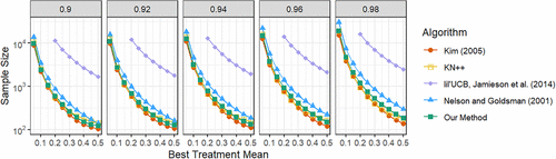
Note. transformed.
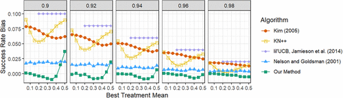
Figure 2 shows that our method is competitive in terms of sample size, and Figure 3 shows that our success rate meets the specified P(CS) as , in accordance with Theorem 1. As grows, our observed success rate dips slightly, partly because of bias from sequential updates to the variance, where earlier-than-optimal stopping can occur because of chance errors in the sample variance estimate. However, the success rate stays within Bradley’s liberal criterion of a 2.5% range around the target rate (Bradley 1978). This shows that our approach deviates little from the error rate guarantees, even in the nonasymptotic condition.
Among the R&S algorithms, Kim (2005) tends to sample slightly less than ours, and KN++ (Kim and Nelson 2006) samples around the same amount, whereas Nelson and Goldsman (2001) consistently sample somewhat more. Despite sampling slightly less than us, we argue that our superior performance in other dimensions can make our approach more practical and desirable than Kim’s for many digital experimentation applications. We discuss these metrics next.
5.2.2. Sample Size Variation.
Sample size standard deviation is a critical metric, as it measures an algorithm’s tendency to over- or undersample with respect to the objective. Many methods perform well on average but suffer from large upper-tail behavior, regularly sampling far more than necessary. We plot the standard deviation of the sample size (Figure 4) and the quantile across simulations to represent the upper tail (Figure 5). Note that the y-axis here is also transformed using the scale. These graphs show that our approach achieves far smaller variation in sample size relative to others.
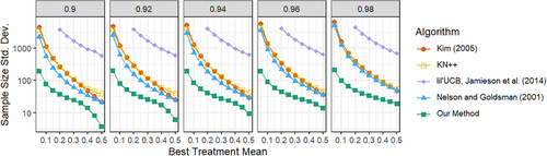
Note. transformed.
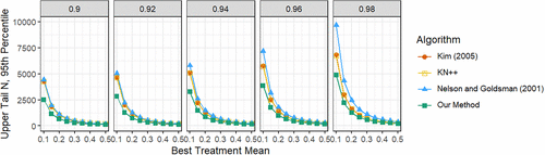
5.2.3. Effect Estimation Bias.
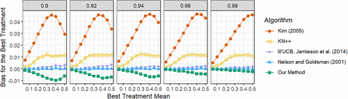
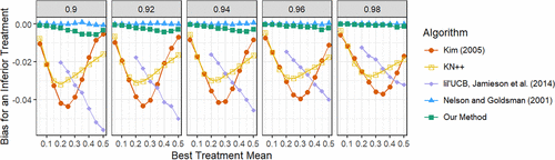
As Nie et al. (2018) demonstrate, adaptive sampling procedures bias the sampled data. Bias in the samples reduces the reliability of the data for post hoc analyses, like heterogeneous effect discovery, worsening data scarcity. However, not all sampling procedures are biased in the same way, and some bias the data far less than others. Here, we compare the methods in terms of the bias in the average outcome estimates for the best treatment and an inferior alternative treatment. Figure 6 and Figure 7 show the estimation bias results.
Usually, bias is introduced when an algorithm uses sample mean information to make sampling decisions. Nelson and Goldsman (2001) never use sample means to decide which arm to sample or how much. Thus, their sample mean estimates are unbiased, and their performance serves as a benchmark. Kim (2005), KN++ (Kim and Nelson 2006), and lil’UCB (Jamieson et al. 2014) are highly adaptive procedures, using the sample mean information at every step to decide whether to continue sampling. This is beneficial when the primary objective is to stop early, but can greatly bias the sample. Our approach takes a middle ground, where the sample mean information is used once at the conclusion of each phase. This reduces how much the inferior treatments are sampled relative to Nelson and Goldsman (2001), while taking on less bias than highly adaptive algorithms such as Kim (2005) and Jamieson et al. (2014).
Kim (2005)’s method exhibits substantial bias for all arms—substantial positive bias for the acceptable arm and substantial negative bias for the unacceptable ones (compounding the bias on the difference in treatment outcomes, which is often of interest in post hoc analysis). KN++ shows bias in some cases but is generally reduced relative to Kim (2005). In comparison, our method shows a relatively small amount of negative bias for all arms.
The difference in the direction of bias of the best arm between our method and the others is also because of adaptivity differences. Kim, KN++, and lil’UCB will stop sampling at any time when one treatment mean is substantially greater than the others. This results in many cases where sampling ends when the best treatment’s sample mean was biased positively because cases where the sample mean was not biased positively lead to more samples, reducing bias. In contrast, our bias largely comes from the cases where the best treatment mean is not selected as the best at the end of phase I, occurring because of negative errors in estimation in phase I. This results in a small portion of samples with negative bias, which, in turn, bias the sample means across simulation runs.
5.3. Performance Comparisons with Non–Normally Distributed Outcomes
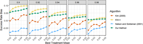
Our method requires only mild moment conditions and does not assume a specific outcome distribution. As a result, it can be applied in a wide range of experimental settings common in digital experimentation, including binary outcomes. Some of the methods we compare against require more stringent assumptions, and their performance is expected to suffer in very nonnormal conditions (e.g., Nelson and Goldsman (2001) and Kim (2005) assume normality). In contrast, methods making a more general distributional assumption should be unaffected, such as Jamieson et al. (2014), which makes a sub-Gaussian assumption on the outcomes, and KN++ (Kim and Nelson 2006), which uses asymptotics and an adapted CLT, akin to our approach. Figure 8 shows P(CS) results for Bernoulli outcomes. We provide further empirical comparisons with these methods in conditions with gamma- and Bernoulli-distributed outcomes in Online Appendix C.3. In general, all methods perform reasonably well in the gamma-distributed condition, whereas only our method and KN++ are able to maintain their statistical guarantees in the Bernoulli-distributed conditions.
5.4. Online Marketing Experiment Demonstration
We partnered with a marketing team that was testing five different ways of advertising an advanced business school degree program. Each advertisement was displayed to several thousand individuals on the web, and the number of individuals who clicked an ad was recorded. Each event where an individual sees an ad is an “impression.” The marketing team sought to determine which ad generated the highest click rate . All click rates (and differences between them) are small, as is typical in digital experiments. Because the marketing campaign was completed before our partnership, we treat the observed data and its click rates as populations from which to sample. We sampled from the click outcomes for each treatment to simulate a sequential experiment on binary outcomes and select the best of the five ads. We repeated the experiment 10,000 times per condition to estimate the mean and variance of the final sample size and observed P(CS).
As discussed previously, for Bernoulli distributions with small p as in this data set, the sample mean converges in distribution to the normal distribution at a slower rate, so we use samples. Note that this is far below the number of samples taken per arm in the first round of MAB methods, such as the median elimination algorithm of Even-Dar et al. (2006) for the small effect sizes in this context.
We suppose that the marketing team has a minimum performance expectation (derived from the break-even expectations balancing ad cost and click value) of one click in 200 impressions, or a click rate of 0.005. They then use this as a baseline performance expectation, which treatment alternatives must dominate (). We then power to detect a superior (acceptable) ad achieving 1.2 clicks out of 100 impressions (), they are willing to budget to distinguish between alternatives as close as 0.004 clicks/impressions (),3 and they seek a correct selection rate of 0.9 ().
|

Table 1. Summary of Design Parameters
| Parameter | Description |
|---|---|
| Input | Specified by the experimenter |
| K | Number of alternative treatments/policies. |
| Target Type I and Type II error probabilities | |
| Practical significance margin for comparison with standard | |
| Lower bound of the indifference zone for selecting best alternative (). | |
| Baseline mean performance (standard/business as usual) | |
| , | Pilot sample sizes (default of 30, higher when normal approximation requires more). |
| , | Sampling step sizes for phase I and II. Default is one. |
| Derived | Calculated via the dp-select procedure conditional on the input parameters |
| Design parameters controlling phase I sampling and stopping rules | |
| Design parameters controlling phase II sampling and stopping rules |
|
Table 2. Error Rate and Sample Size Estimates for Our Method in Simulation
| K | Type I error | P(CS) | |||||||||||
|---|---|---|---|---|---|---|---|---|---|---|---|---|---|
| 0.1 | 0.5 | 2 | 0.05 | 0.8 | 3 | 3 | 292.6 | 293.7 | 50.6 | 0.0539 | 0.790 | ||
| (24.4) | (17.7) | (16.8) | |||||||||||
| 0.1 | 0.5 | 2 | 0.05 | 0.8 | 10 | 3 | 3,260.8 | 294.0 | 553 | 0.0517 | 0.799 | ||
| (81.5) | (7) | (182) | |||||||||||
| 0.1 | 1.0 | 2 | 0.05 | 0.8 | 3 | 3 | 73.2 | 74.5 | 28 | 0.0531 | 0.799 | ||
| (12.9) | (10) | (7.5) | |||||||||||
| 0.1 | 1.0 | 2 | 0.05 | 0.8 | 10 | 3 | 828.6 | 75.2 | 124 | 0.0491 | 0.804 | ||
| (40.5) | (4.2) | (39.4) | |||||||||||
| 0.1 | 0.5 | 3 | 0.05 | 0.8 | 3 | 5 | 10 | 379.7 | 1,056.4 | 4,226.8 | 57.6 | 0.0488 | 0.800 |
| (27.7) | (39.9) | (80.2) | (73.3) | ||||||||||
| 0.1 | 0.5 | 3 | 0.05 | 0.8 | 10 | 3 | 5 | 4,225.2 | 381.0 | 1,057.1 | 486 | 0.0497 | 0.802 |
| (91.5) | (7.97) | (19.7) | (140) | ||||||||||
| 0.1 | 1.0 | 3 | 0.05 | 0.8 | 3 | 3 | 3 | 95.6 | 96.9 | 97.2 | 28.7 | 0.0501 | 0.797 |
| (14.5) | (10.8) | (9.06) | (6.05) | ||||||||||
| 0.1 | 1.0 | 3 | 0.05 | 0.8 | 3 | 5 | 10 | 96 | 268 | 1,076 | 29.8 | 0.0534 | 0.793 |
| (14.7) | (20.9) | (40.7) | (11.7) | ||||||||||
| 0.1 | 1.0 | 3 | 0.05 | 0.8 | 10 | 3 | 5 | 1,074.4 | 97.5 | 269.5 | 106 | 0.0453 | 0.798 |
| (46.3) | (4.07) | (10.2) | (29.9) |
Table 3 shows the results of these experiments. For this demonstration, we assume the empirically best treatment in the full data set is the true best, so “success” is defined as selecting that treatment. In the case of binary rather than normal outcomes, we observe a higher rate of correct selection than desired, which means that our sample size is somewhat larger than is necessary, although this is because of, at least in part, the “population” p values being in a position that is slightly easier to detect than the LFC (because the inferior ps are not all exactly equal to ; some are smaller). Contrast this with the median elimination (Even-Dar et al. 2006) and exponential-gap (Karnin et al. 2013) algorithms: for an experiment with desired and indifference margin of 0.004, median elimination samples (using the natural log) observations from each treatment in the first round alone. The exponential-gap algorithm uses median elimination as a subroutine, and by the third iteration, exponential gap generally eliminates no alternatives (including the standard), and the first round of the median elimination subroutine draws nearly three million samples per arm.
|
Table 3. Results from Analysis of Digital Ad Experiment Data
| Specified P(CS) | 0.9 | 0.92 | 0.94 | 0.96 | 0.98 |
|---|---|---|---|---|---|
| Mean sample size | 10,835 | 11,968 | 13,585 | 15,903 | 19,759 |
| Observed P(CS) | 0.967 | 0.972 | 0.981 | 0.992 | 0.997 |
Notably, the original experiment consisted of 123,840 impressions across all treatments. Thus, with these small effect sizes and stringent error rate requirements, we sample substantially less than the original experiment.
6. Conclusion
Our sequential method for determining the best treatment is a pragmatic approach that maps closely to a managerial need in digital experimentation: well-powered experiments when participants are scarce. This approach is designed to use near the ideal sample size, the exact number of samples implied by an experimenter’s objectives with respect to error rates ( and ) and effect margins ( and ), and the sequential estimation of the necessary sample size results in substantially less over- or undersampling than competitor methods. Unlike many other methods in this space, our method requires no hyperparameter tuning: the design parameters correspond directly to the experimenter’s preferences and objectives, whereas the derived design parameters (, , , and ) are provided by our optimization routine dp-select. Our sequential selection method and procedure for finding the design parameters are implemented in an R package.4
The Monte Carlo simulation studies demonstrate that our method is competitive with existing approaches in terms of sample size and superior in terms of sample size precision. The simulations also show that estimation bias is less than Kim (2005) and Kim and Nelson (2006), the comparison methods that are most competitive in terms of sample size. Monte Carlo studies also validate that our method is just as effective in nonnormally distributed conditions when starting sample sizes (, ) are large enough to engage the central limit theorem, whereas some of our competitors do not adapt as easily. Simulations with gamma-distributed populations show resilience to skewness, and simulations with small-p binary data and a study based on data from a real digital experiment show effectiveness given small-p binary outcomes.
Despite its applicability, stopping rule–based methods such as ours can produce practical challenges for experimenters. A primary challenge is that it is possible that the stopping rule is prohibitively out of reach—far beyond the sample budget of the experimenter. This is essentially the case for all R&S and MAB methods we discussed. However, the simplicity of our stopping rule allows experimenters to estimate the remaining sample size needed, and this feature is implemented in our R package. Once the sample size is high enough to have a reasonably precise estimate of the sample variance, it is unlikely that the estimated sample size will change dramatically. It is up to the experimenter’s discretion to stop early in this case. If stopping is done solely based on the projected sample size being well estimated at a prohibitively large value, the samples are not contaminated. In other words, early stopping in this case does not prohibit the further usage of those samples, although the result of our method must be a failure to reject the null hypothesis in that case.
One limitation of our approach relative to the highly adaptive sampling methods such as Kim (2005), Kim and Nelson (2006), and Jamieson et al. (2014) is that we will generally not stop poorly performing treatments as early. This is a direct trade-off with the low sample size variance and low effect estimate bias, both of which generally increase with adaptivity. If an experimenter has a prior belief that most of the treatments are poor, one of these may be a preferable approach. However, in digital experimentation, very small differences between treatments are quite common, as evidenced by the digital experiment field data analyzed in Section 5.4.
Additionally, our method assumes a known baseline treatment, representing a known business-as-usual mean outcome or baseline performance expectation. In some applications, an experimenter may have no baseline performance expectation and have only a noisy estimate of the business-as-usual condition. Adapting our method to use an estimated baseline would make a valuable extension of our work that would require a generalized form of Theorem 1 for such conditions. In lieu of this advancement, experimenters might use an optimistic estimate or upper confidence interval value as to form a conservative test.
Although we propose a particular method in this work, the managerial problem of balancing scarcity and test power is broader than the problem of selection among alternatives. Experimenters employ a broad set of tests, from simple A/B tests to customer subgroup heterogeneity analyses. Future method development in these domains should increasingly focus on precisely balancing power and resource usage.
1 Another case of note: for several i, , and . By the experimenter’s preference, all of these treatments are acceptable and so close to each other that they are not worth distinguishing, so selecting and rejecting with any of them results in success. The power will be greatly increased relative to the LFC in this case.
2 Following a note in Kim and Nelson (2006), we adjust KN++ for the finite-sample setting by using hyperparameter values designed for the KN+ algorithm, leading it to sample somewhat more and ensure it achieves its error rate guarantees in our settings.
3 This margin preference is close to the difference between the best and second-best means presented by the data, assuming that the estimated ’s from the actual study are the true parameters in our simulation. This allows us to show that our correct selection rate at the LFC is close to the desired rate, and each method uses this margin in the simulation.
4 Our R package can be freely accessed in the GitHub repository at https://github.com/will-stamey1/seqbest.
References
- (2025) The critical challenge of using large-scale digital experiment platforms for scientific discovery. MIS Quart. 49(1):1–28.Crossref, Google Scholar
- (2015) Sequential and two-stage fixed-width confidence interval estimation in response-adaptive designs. Sequential Anal. 34(3):350–363.Crossref, Google Scholar
- (2022) A non-asymptotic approach to best-arm identification for Gaussian bandits. Proc. 25th Internat. Conf. Artificial Intelligence Statist., vol. 151 (PMLR, New York), 10078–10109.Google Scholar
- Berman R, Pekelis L, Scott A, Van den Bulte C (2018) p-Hacking and false discovery in A/B testing. Preprint, submitted July 18, https://ssrn.com/abstract=3204791.Google Scholar
- (2022) Online experimentation: Benefits, operational and methodological challenges, and scaling guide. Harvard Data Sci. Rev. 4(3):235–244.Google Scholar
- (2023) Design and analysis of switchback experiments. Management Sci. 69(7):3759–3777.Link, Google Scholar
- (1978) Robustness? British J. Math. Statist. Psych. 31(2):144–152.Crossref, Google Scholar
- (2016) Estimation of the coefficient of variation with minimum risk: A sequential method for minimizing sampling error and study cost. Multivariate Behav. Res. 51(5):627–648.Crossref, Google Scholar
- (2012) Sequential sampling with economics of selection procedures. Management Sci. 58(3):550–569.Link, Google Scholar
- (1988) Statistical Power Analysis for the Behavioral Sciences, 2nd ed. (Routledge, New York).Google Scholar
- (2020) Gini index estimation within pre-specified error bound: Application to Indian household survey data. Econometrics 8(2):26–45.Crossref, Google Scholar
- (2002) PAC bounds for multi-armed bandit and Markov decision processes. Kivinen J, Sloan RH, eds. Comput. Learn. Theory. COLT 2002, Lecture Notes in Computer Science, vol. 2375 (Springer, Berlin, Heidelberg), 255–270.Google Scholar
- (2006) Action elimination and stopping conditions for the multi-armed bandit and reinforcement learning problems. J. Machine Learn. Res. 7(39):1079–1105.Google Scholar
- (2016) Indifference-zone-free selection of the best. Oper. Res. 64(6):1499–1514.Link, Google Scholar
- (2019) Test & roll: Profit-maximizing A/B tests. Marketing Sci. 38(6):1038–1058. Link, Google Scholar
- (2016) Optimal best arm identification with fixed confidence. 29th Annual Conf. Learn. Theory, vol. 49 (PMLR), 998–1027.Google Scholar
- (2022) Smooth contextual bandits: Bridging the parametric and nondifferentiable regret regimes. Oper. Res. 70(6):3261–3281.Link, Google Scholar
- (2014) lil’ UCB: An optimal exploration algorithm for multi-armed bandits. Balcan MF, Feldman V, Szepesvári C, eds. Proc. 27th Conf. Learn. Theory, vol. 35 (PMLR, New York), 423–439.Google Scholar
- (2017) Peeking at A/B tests: Why it matters, and what to do about it. KDD’17: Proc. 23rd ACM SIGKDD Internat. Conf. Knowledge Discovery Data Mining (Association for Computing Machinery, New York), 1517–1525.Google Scholar
- (2021) Always valid inference: Continuous monitoring of A/B tests. Oper. Res. 70(3):1806–1821.Link, Google Scholar
- (2018) Editor’s comments: Opportunities and challenges for different types of online experiments. MIS Quart. 42(4):iii–x.Crossref, Google Scholar
- (2013) Almost optimal exploration in multi-armed bandits. Dasgupta S, David McAllester D, eds. Proc. 30th Internat. Conf. Machine Learn., vol. 28 (PMLR, New York), 1238–1246.Google Scholar
- (2018) Accuracy in parameter estimation for a general class of effect sizes: A sequential approach. Psych. Methods 23(2):226–243.Crossref, Google Scholar
- (2005) Comparison with a standard via fully sequential procedures. ACM Trans. Model. Comput. Simulation 15(2):155–174.Crossref, Google Scholar
- (2006) On the asymptotic validity of fully sequential selection procedures for steady-state simulation. Oper. Res. 54(3):475–488.Link, Google Scholar
- (2022) A/B testing intuition busters: Common misunderstandings in online controlled experiments. KDD’22: Proc. 28th ACM SIGKDD Internat. Conf. Knowledge Discovery Data Mining (Association for Computing Machinery, New York), 3168–3177.Google Scholar
- (2013) Online controlled experiments at large scale. KDD’13: Proc. 19th ACM SIGKDD Internat. Conf. Knowledge Discovery Data Mining (Association for Computing Machinery, New York), 1168–1176.Google Scholar
- (2022) Experimentation and start-up performance: Evidence from A/B testing. Management Sci. 68(9):6434–6453.Link, Google Scholar
- (2004) The sample complexity of exploration in the multi-armed bandit problem. J. Machine Learn. Res. 5:623–648.Google Scholar
- (2008) Sample size planning for statistical power and accuracy in parameter estimation. Annual Rev. Psych. 59:537–563.Crossref, Google Scholar
- (2025) An investigation of p-hacking in e-commerce A/B testing. Inform. Systems Res. 36(3):1691–1717.Link, Google Scholar
- (2009) Sequential Methods and Their Applications (CRC Press, Boca Raton, FL).Google Scholar
- (2001) Comparisons with a standard in simulation experiments. Management Sci. 47(3):449–463.Link, Google Scholar
- (1934) On the two different aspects of the representative method: The method of stratified sampling and the method of purposive selection. J. Roy. Statist. Soc. 97(4):558–625.Crossref, Google Scholar
- (2018) Why adaptively collected data have negative bias and how to correct for it. Storkey A, Perez-Cruz F, eds. Proc. 21st Internat. Conf. Artificial Intelligence Statist. (AISTATS), vol. 84 (PMLR, New York), 1261–1269.Google Scholar
- (2005)
A two-stage design for choosing among experimental treatments in clinical trials . Balakrishnan N, Nagaraja HN, Kannan N, eds. Advances in Ranking and Selection, Multiple Comparisons, and Reliability, Statistics for Industry and Technology (Birkhäuser, Boston), 385–409.Crossref, Google Scholar - (2017) Customer acquisition via display advertising using multi-armed bandit experiments. Marketing Sci. 36(4):500–522.Link, Google Scholar
- (1988) Two-stage selection and testing designs for comparative clinical trials. Biometrika 75(2):303–310.Crossref, Google Scholar
- (2013) Sequential Bayes-optimal policies for multiple comparisons with a known standard. Oper. Res. 61(5):1174–1189.Link, Google Scholar
- (2024) Optimal experimental design for staggered rollouts. Management Sci. 70(8):5317–5336.Link, Google Scholar
- (2023) Adaptive Neyman allocation. Preprint, submitted September 15, https://arxiv.org/abs/2309.08808.Google Scholar
Will Stamey is a fifth-year PhD candidate in analytics at the University of Notre Dame Mendoza College of Business. His research develops computational statistics and machine learning methodologies to meet managerial challenges in decision making in high-frequency and high-dimensional data. His work especially focuses on the algorithmic discovery of effective treatments or the detection of treatment-sensitive subpopulations in causal inference, which can guide policy rollout decisions and treatment personalization.
Ken Kelley is the Sorin Society Professor of IT, Analytics, and Operations at Notre Dame. His work spans the development and application of methods for study design, construct measurement, and the analysis of data in human-centered research. His most impactful work is on sample size planning, confidence interval formation, and effect-size estimation. As an R developer, he builds software that makes these and other methods accessible to researchers. Kelley codirects the Human-centered Analytics Lab.
Bhargab Chattopadhyay is an associate professor in the area of information systems and analytics at the School of Management and Entrepreneurship at Indian Institute of Technology Jodhpur. His research spans sequential analysis, digital experimentation, and statistical inference, with applications in methodological statistics, econometrics, information systems, and marketing. He serves as an associate editor of the journal Sequential Analysis. Prior to IIT Jodhpur, he worked at the University of Texas at Dallas and the Indian Institute of Management Visakhapatnam.
Tathagata Bandyopadhyay is the director general of Dhirubhai Ambani University, Gandhinagar, India. He received his PhD in statistics from the University of Calcutta. His research interests include statistical inference, measurement error models, discrete data modeling, and machine learning. He has authored numerous publications in leading national and international journals and has served the academic community in various editorial roles. His current research focuses at the intersection of statistics and artificial intelligence.

