Honesty in Causal Forests: When It Helps and When It Hurts
Abstract
Causal forests estimate how treatment effects vary across individuals, guiding personalized interventions in areas like marketing, operations, and public policy. A standard practice is honest estimation—dividing the data into two samples, one to define subgroups and another to estimate treatment effects within them. This is intended to reduce overfitting and is the default in many software packages. But is it the right choice? We show that honest estimation can reduce the accuracy of estimates of individual treatment effects—especially when effect heterogeneity is substantial and data sets are large enough to detect it. The reason is a bias-variance trade-off: honesty lowers the risk of overfitting but increases the risk of underfitting by limiting the data available to detect and model heterogeneity. Across more than 7,000 benchmark data sets, we find that the cost of using honesty by default can be as high as requiring 27% more data to match the performance of models trained without it. Honesty is best understood as a form of regularization. Whether to adopt it should depend on the goals of the application and its empirical performance, not on reflexive default use.
History: Ravi Bapna, Senior Editor; Mochen Yang, Associate Editor.
Supplemental Material: The online appendix is available at https://doi.org/10.1287/isre.2025.2343.
1. Introduction
Some modeling choices become standard practice not because they are optimal, but because they are conservative, familiar, and built into the tools we use. But in applied settings, such defaults can come at the expense of making effective use of our data.
Causal forests provide a prominent example of this tension. They are a popular method for estimating how treatment effects vary across individuals (Wager and Athey 2018) and are increasingly used in fields such as marketing, operations, economics, and public policy to support personalization and targeting. Since 2019, dozens of papers in INFORMS journals have applied causal forests to experimental or observational data (see Online Appendix J), often as part of broader analytics pipelines that rely on individual-level effect estimation.
The method mirrors random forests for outcome prediction, but with causal effects as the target. Another key difference lies in how the data are used. Standard random forests use the full training sample to both build trees and estimate leaf-level predictions. Causal forests often divide the data in two: one part to form leaves, and another to estimate leaf-level effects. This practice—known as honest estimation or honesty—is the default in widely used software packages such as grf (Athey et al. 2019) and EconML (Battocchi et al. 2019), and is commonly recommended in applied work. But is this default a good idea?
On the one hand, honesty can help by preventing the same sampling error from influencing both leaf formation and effect estimation, reducing overfitting and selection bias (Athey and Imbens 2016a). On the other hand, it can hurt because it reduces the data available to form leaves and estimate effects.
We examine this trade-off in the context of estimating individual treatment effects as accurately as possible, a central concern in personalization and targeting applications. In this setting, honest estimation acts as a form of regularization: by constraining how much the model can adapt to the data, it trades flexibility for stability, much like other regularization choices. This trade-off can lead to less accurate models when effects differ substantially across individuals and the data set is large enough to detect those differences.
To support this claim, we analyze how honesty affects the bias-variance trade-off in estimating individual treatment effects, both analytically and empirically. We find that its use of separate subsamples reduces variance, but the smaller subsample sizes limit the detection of heterogeneity and increase bias.
Our empirical analysis is based on 7,500 benchmark data sets from the Atlantic Causal Inference Conference (ACIC) (Dorie et al. 2019), covering a wide range of settings that vary in how difficult it is to model effect heterogeneity. The findings align with the mechanisms highlighted by our analytical results. Honesty works reasonably well when differences in effects are small or difficult to detect, but can backfire when heterogeneity is more pronounced. In such settings, honest estimation can require up to 27% more data to achieve the same level of accuracy as causal forests learned without it.
This paper makes three contributions. First, we show that treating honest estimation as a default is unwarranted, as it can degrade accuracy when effect heterogeneity is substantial and detectable in the data. Second, we explain why this occurs by interpreting honesty as a form of regularization that governs a bias-variance trade-off. Third, we show that the choice between honest and nonhonest estimation can matter substantially in practice, and offer concrete guidance on when to use each.
2. How Tree-Based Causal Estimation Works
This section defines the algorithm we consider for estimating treatment effects. We begin with a single tree, specifying how subpopulations are formed and how effects are estimated, and then extend to forests. Online Appendix I reviews the broader development of causal forests and honest estimation in the literature.
2.1. Setup and Causal Quantities
Consider the standard setup in which each individual is described by a feature vector (e.g., age, income), a binary treatment assignment , and an outcome Y. Each individual has two potential outcomes— if treated and if not—but we only observe one of them,
We assume that treatment is assigned uniformly at random, so ignorability holds,
This means differences in outcomes between treated and control individuals can be interpreted causally. Our object of interest is the individual treatment effect (ITE),
A tree estimates by dividing the feature space into subpopulations (leaves) and estimating the average effect within each one. Let denote a leaf. The subpopulation average treatment effect (SPATE) of is
Given an estimation sample , the tree estimates the SPATE by comparing the average outcomes of treated and control units:
2.2. How Subpopulations Are Chosen
We want subpopulations such that the SPATE closely approximates the CATEs of individuals with . A subpopulation is therefore “good” if effects vary little within it. For any candidate leaf , we measure this using the approximation’s mean squared error (MSE),
Learning the tree then amounts to recursively finding splits that reduce this within-leaf error. For a split of a parent node into children and , the MSE gain is
The tree learner uses a splitting sample and the following criterion to estimate this gain:
We denote by the leaf assignment of an individual under the tree partition learned from .
2.3. Effect Estimation
Given a splitting sample and an estimation sample , the tree assigns an individual to a leaf and uses the corresponding SPATE estimate as the individual’s effect:
Under honest estimation (HE), the data are divided so that and are disjoint subsamples. Under adaptive estimation (AE), all the data are used for both leaf formation and effect estimation, so .
A causal forest extends this by aggregating estimates across many trees, each constructed from a different subsample of the training data. Let denote B subsamples drawn without replacement. The prediction of the tree trained on subsample is
The forest prediction is the average of these tree predictions:
3. A Bias-Variance Perspective
To unpack the trade-off between HE and AE, we analyze how each affects the bias and variance of causal forest estimates. For a given individual with CATE , the MSE decomposes as
Our goal is not to derive precise conditions under which HE dominates AE, or vice versa. The choice between the two should be guided empirically, as discussed in Section 4. Instead, we use the bias-variance decomposition to clarify how honesty affects the accuracy of CATE estimates.
Because the bias and variance of a causal forest arise from aggregating individual trees, we begin by understanding the errors made by a single tree:
3.1. Where Bias Comes From
The bias of a causal forest coincides with the bias of its individual trees. Taking expectations,
Using the decomposition in Equation (14), we can write tree bias as the sum of its expected approximation and estimation errors:
Estimation bias arises under AE because the same data are used to select splits and estimate effects. The tree learner searches over many candidate splits and chooses those that appear to best separate individuals by treatment effects, even when that separation reflects sampling error rather than true heterogeneity. As a result, SPATE estimates under AE are systematically exaggerated—an instance of selection bias—with above-average effects biased upward and below-average effects biased downward.
HE eliminates estimation bias by construction. By using separate samples for splitting and estimation, leaf assignments and effect estimates become independent. Even if some splits are chosen because of sampling error, the effect estimate within each leaf remains unbiased:
However, data splitting under HE increases approximation bias. With fewer data to evaluate candidate splits, the tree learner has a harder time identifying informative features, so the resulting subpopulations may align less closely with heterogeneity in treatment effects.
The implication is that HE and AE trade off approximation and estimation bias in opposite ways. Empirically, we find that AE wins in this trade-off. We illustrate this next with a simple analytical example.
3.2. A Stylized Example of Bias
Consider a deliberately simple setting—a tree with a single split—designed to cleanly isolate the sources of bias. Formal derivations are in Online Appendix B.
Suppose is a vector of binary features. Exactly one feature, , is informative about treatment effects:
Individuals with benefit from treatment, whereas those with are harmed by the same amount. All remaining features serve only as noise. The average treatment effect in the population is zero.
Individual effects are estimated using a tree with a single split. If the tree splits on the feature , the resulting leaves align perfectly with true effect heterogeneity. If it splits on any other feature, both leaves have the same SPATE—equal to zero—and are therefore uninformative.
Consider an individual with , for whom the CATE is (the case is symmetric). The superscripts H and A distinguish HE and AE quantities, and denotes splitting on . As discussed earlier, HE has no estimation bias, so leaf-level (SPATE) estimates are unbiased:
However, HE is still biased for CATE estimation because it may split on a noninformative feature. Taking expectations over splits,
The resulting bias is
Now consider AE. When the tree splits on a noninformative feature (), the actual SPATE in both leaves is zero. AE systematically exaggerates the SPATE estimates, but the errors are symmetric around zero and cancel out in expectation, so there is no estimation bias:
Things play out differently when AE splits on the informative feature (). Sampling error can make this split look more or less informative than it truly is, and the tree learner is more likely to select it when the error is favorable. Conditioning on therefore selects cases where the estimation error is positive or not too negative—this is the selection bias discussed earlier. Because AE uses the same data for splitting and estimation, this bias carries over to the leaf estimates, leading to upward bias:1
AE’s advantage is that it splits on the informative feature more often than HE,
This means AE accepts some estimation bias in exchange for lower approximation bias. Its overall bias is negative and always smaller than that of HE in this example:
Figure 1 illustrates this trade-off.
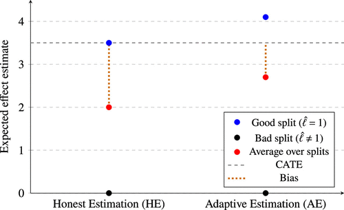
Notes. HE is unbiased conditional on a correct split, whereas AE exhibits selection bias. However, AE selects the informative feature more often, reducing approximation bias and producing an estimate closer to the CATE in expectation.
3.3. Where Variance Comes From
We now turn to the variance of a causal forest. Because a forest averages predictions across trees, its variance corresponds to the average of tree covariances:
As the number of trees grows, the dominant contribution comes from cross-tree covariances, for . Understanding forest variance therefore reduces to understanding the sources of dependence between tree predictions.
We first decompose each tree prediction into the two components introduced in Equation (14): an approximation target and an estimation error. Tree b assigns to a leaf , which defines a SPATE
This is the approximation target. The corresponding prediction is
We then decompose the covariance between tree predictions as
This decomposition reveals three distinct sources of dependence. We discuss each in turn and provide analytical derivations to support our arguments in Online Appendix C.
3.3.1. Target Coupling.
, captures dependence across trees arising from variability in their approximation targets. To build intuition, consider the stylized example from Section 3.2. A tree may sometimes split on the informative feature, producing leaves that reflect true effect heterogeneity, and sometimes fail to do so, producing uninformative leaves. Which occurs depends on the specific training sample. Because trees are grown on overlapping subsamples, they tend to succeed or fail together. This shared fate induces covariance between their approximation targets.
HE affects target coupling indirectly by reducing the size of the splitting sample, limiting trees’ ability to identify good approximation targets. Whether this increases or decreases target coupling depends on the signal-to-noise ratio (SNR): how easy it is to infer variation in treatment effects from data.
When informative features are easy to identify (high SNR), HE disrupts otherwise reliable splits, making approximation targets more sensitive to the training sample and increasing target coupling. When informative features are difficult to detect reliably (low SNR), trees find good approximation targets only inconsistently. HE stabilizes them by removing those unreliable attempts, reducing target coupling—though at the cost of also missing the occasional good split. Figure 2 illustrates this effect in our stylized example.
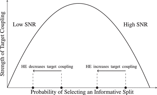
Notes. HE decreases the probability of an informative split compared with AE. In high-SNR settings (right), this moves trees away from reliable and informative splits, increasing sampling sensitivity and target coupling. In low-SNR settings (left), the same shift moves trees toward stable, uninformative targets and reduces target coupling.
Empirically, however, we find that HE produces lower target coupling than AE even when SNR is high.
3.3.2. Target-Estimation Dependence.
Target-estimation dependence is the source of variance that honesty is designed to address. This dependence arises when the same sampling error that favors a split also biases the estimated SPATE in the same direction: above-average SPATEs are more likely to be overestimated, whereas below-average SPATEs are more likely to be underestimated. This introduces a dependence between the approximation target and the estimation error that inflates variance.
By separating the samples used for splitting and effect estimation, HE breaks this dependence within a tree, so the estimation error has conditional mean zero given the leaf assignment:
This rules out target-estimation dependence within a tree, but not at the forest level. Trees are trained on overlapping subsamples of the same data, so observations in one tree’s estimation sample may appear in another’s splitting sample. Therefore, the estimation error of one tree may correlate with the approximation target of another, resulting in the target-estimation spillover in Equation (28).
To eliminate this dependence entirely, the approximation target of each tree must be independent of the estimation error across all trees.2 Under full independence,
We refer to this idealized condition as forest honesty. Although honest causal forests do not satisfy forest honesty exactly, they are designed to approximate it by separating target selection from effect estimation, and thus more closely adhere to this condition than adaptive forests. Assumptions of this kind are common in the theoretical analysis of tree-based methods, where they are introduced to simplify dependence and make analysis tractable. For example, Scornet (2016) studies forests with data-independent (uniform) splitting, and Klusowski (2021) uses midpoint splitting rules.
Forest honesty plays the same role here. We next analyze the covariance decomposition in Equation (28) under this abstraction to isolate the effect of reducing target-estimation dependence.
3.3.3. How Honesty Reduces Overfitting.
Under forest honesty, the target-estimation spillover terms in Equation (28) disappear:
This leaves noise overlap, , which arises because different trees may reuse the same observations in their estimation samples, introducing correlation in their estimation errors. It has two components:
The first is unavoidable and depends primarily on sample size and how similar the leaves are across trees. Smaller samples and more similar leaves imply greater overlap. Because forests average over many trees, the reduced estimation sample size induced by HE does not affect this component asymptotically.
The second arises from target-estimation dependence. The same sampling error that makes a partition look informative in one tree is likely to make it look informative in other trees too. When those noisy observations are reused for estimation, as under AE, it induces additional correlation between estimation errors. Under forest honesty, this component vanishes, reducing variance.
3.4. Summary
Estimating individual treatment effects with trees involves two sources of error: approximation error, from summarizing effects within leaves, and estimation error, from sampling variability and selection bias in estimating those leaf-level effects. HE and AE trade off these errors differently.
HE eliminates estimation bias by separating the data used for splitting and estimation, but increases approximation bias by limiting trees’ ability to detect effect heterogeneity. AE accepts some estimation bias in exchange for lower approximation bias, which leads to lower overall bias.
At the forest level, variance arises from dependence across trees. HE reduces variance by breaking the link between sampling error in split selection and effect estimation. In high-SNR settings, it can theoretically increase variance by destabilizing otherwise reliable splits, but we do not observe this empirically.
Overall, honesty acts as a form of regularization: more bias, less variance. Theory predicts it helps when SNR is low and hurts when it is high.
4. Empirical Study
This section addresses three practical questions. First, how should a practitioner choose between HE and AE? Second, how much does that choice matter? Third, do their performance patterns match the bias-variance mechanisms developed earlier?
To mirror applied settings where treatment effects are unobserved, we adopt a fully data-driven workflow. We tune HE and AE via cross-validation using transformed outcomes (Athey and Imbens 2015) as effect proxies, and then evaluate performance using ground-truth CATEs. We also quantify what the choice costs by asking how much additional data one approach requires to match the other.
4.1. Benchmark Data
We evaluate HE and AE using the 2016 ACIC benchmarking suite (Dorie et al. 2019), which was created for a competition to compare causal estimators. The benchmark consists of semisynthetic data sets that combine real covariates from the Infant Health and Development Program (IHDP) with simulated treatment assignments and potential outcomes, providing ground-truth CATEs for each individual.
The suite includes 77 distinct types of data-generating processes (DGPs). Within each type, 100 data sets are generated by varying the underlying parameters. We exclude data sets with no treatment effect heterogeneity, yielding 7,500 data sets for analysis. Each data set contains 4,802 observations and 58 covariates. The DGPs vary widely in functional form, complexity, and the strength of treatment effect heterogeneity, so the benchmark is well suited to study the HE-AE trade-off in a multitude of conditions. The data sets were originally designed to study causal estimation under confounding, so we reassign treatment uniformly at random to isolate the task of modeling effect heterogeneity under clean randomization.
We calculate the SNR for each data set as follows. We define noise as idiosyncratic variation in outcomes,
The SNR for a given data set is
Higher SNR implies treatment effect heterogeneity is stronger and easier to estimate from data.
4.2. Design and Workflow
Our empirical design mirrors applied deployment: treatment effects are unobserved, so model selection must rely on observable quantities. For each data set, we randomly assign treatment with probability 0.5 and split the sample into 4,000 observations for training and 802 for testing.
4.2.1. Tuning.
We tune AE and HE separately using fivefold cross-validation on the training sample.3 The tuning parameter is min_samples_leaf. Because HE uses only half of each subsample for splitting, it requires smaller minimum leaf sizes to attain a comparable number of leaves to AE. The tuning grid for AE is and for HE is (half the AE values).
Because individual CATEs () are unobserved, the tuning relies on the transformed outcome , whose conditional expectation equals the CATE (Athey and Imbens 2015). We select hyperparameters by minimizing the MSE between the predicted CATE () and on the validation set :
4.2.2. Selection.
The comparison between AE and HE only matters when the methods can detect heterogeneity in the first place. Our selection procedure has two steps. First, we create a new fivefold split of the training data—distinct from the one used for tuning—and apply the heterogeneity test of Imai and Li (2025), in its cross-fitting implementation, to both tuned estimators.4 If neither passes, it means the signal is too weak to support reliable effect estimation, so we exclude the data set. If only one passes, we select it. If both pass, we compare their performance using out-of-fold transformed-outcome MSE: we treat HE as the default and select AE only if its MSE is lower by at least one standard error, estimated from the paired differences in squared errors across held-out units.
The asymmetry of the rule is theoretically motivated. HE is expected to outperform AE in low-SNR settings, where the empirical comparison is also least reliable, so we default to HE and let the data overturn that default only when the evidence is strong. The one-standard-error threshold follows a standard selection heuristic (Breiman et al. 1984, Hastie et al. 2009), but it is a conventional choice; other thresholds could be used. Online Appendix D develops the full rationale and shows that performance is robust across thresholds.
4.2.3. Evaluation.
We evaluate performance using a metric we denote , defined in analogy to . Although measures the proportion of outcome variance explained by a predictive model, measures the proportion of explainable treatment effect variance—the signal—captured by a causal model. It is based on the MSE between the predicted and true CATEs:
4.3. Results
Among the 7,500 ACIC data sets, neither tuned forest passes the heterogeneity test in 496 cases. We therefore evaluate AE, HE, and the empirical selector on the remaining 7,004 data sets.
We evaluate our selection strategy using a regret framework. For a given data set, regret measures the loss from using a strategy m instead of the oracle (the best of AE and HE in hindsight):
Average regret decomposes into how often a strategy picks wrongly and how costly those mistakes are:
Table 1 summarizes performance across the 7,004 data sets. AE has lower average regret than HE and is more often the better choice, but its mistakes carry more downside risk. The empirical selector achieves the lowest average regret and reduces the cost of mistakes, but has a higher error rate than AE. Both improvements are statistically significant relative to AE and HE.5
|

Table 1. Selection Performance Across 7,004 ACIC Data Sets
| Method | Error rate | ||
|---|---|---|---|
| Empirical | 0.0124 | 30.71% | 0.0405 |
| AE | 0.0136 (+0.0012**) | 25.20% | 0.0542 (+0.0137***) |
| HE | 0.0344 (+0.0220***) | 74.80% | 0.0460 (+0.0055***) |
Notes. Boldface indicates the lowest value in each column. Values in parentheses report difference relative to the empirical selector; positive values indicate higher regret. Differences in are tested using one-sided paired t-tests across data sets. Differences in are tested with bootstrapping because the conditioning events differ across methods.
**p < 0.05; ***p < 0.01.
To visualize protection against costly mistakes, Figure 3 plots regret percentiles from the 90th to the 99.5th percentile. AE’s advantage over HE persists through most of the range, but its regret rises sharply beyond the 98th percentile. HE protects us from such extreme regret. The empirical selector combines these strengths, capturing most of AE’s gains while reducing its tail risk.
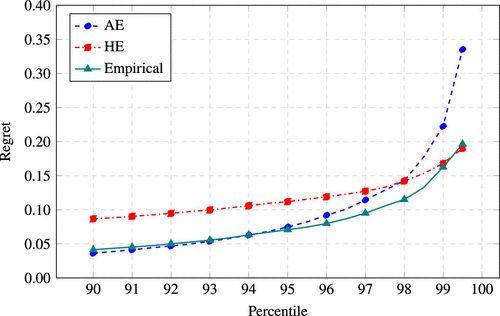
Notes. AE has lower regret than HE across most percentiles but is more vulnerable to extreme regret. The empirical selector captures most of AE’s gains while substantially reducing its tail risk.
Figure 4 breaks down average by SNR decile, where decile 1 contains the weakest-signal data sets and decile 10 the strongest. AE outperforms HE in most deciles, but falls behind in the lowest-SNR regime. This pattern reflects their complementary strengths: AE better exploits heterogeneity when the signal is strong, whereas HE is more reliable when it is weak. The empirical selector closely tracks the better-performing estimator across the full SNR range. It is close to AE in most deciles, nearly coincides with the oracle when SNR is high, and shifts toward HE in the weakest-signal regime.
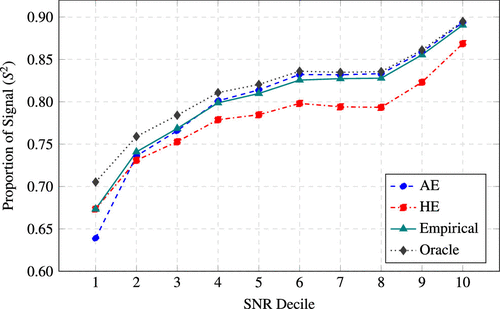
Notes. AE outperforms HE in most deciles but falls behind in the lowest-SNR decile. The empirical selector closely tracks the better-performing method across deciles, nearly coinciding with the Oracle when SNR is high.
We next quantify the practical cost of choosing honesty: how much additional data does HE require to match AE? For each data set, we identify the smallest training size at which the better-performing method still significantly outperforms its alternative (at the 5% level), retuning hyperparameters at each sample size so both methods are evaluated at their optimal complexity (see Online Appendix E for details).
Figure 5 shows the result averaged within each SNR decile. In the lowest-SNR decile, HE achieves comparable performance with roughly 7% fewer data. As SNR increases, the cost of honesty grows, and HE requires up to 27% more data to match AE.
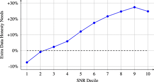
Note. In the lowest-SNR regime, HE requires roughly 7% fewer data than AE, but up to 27% more data as SNR increases.
4.4. Honesty as Regularization
We now test the theoretical interpretation of honesty as regularization, trading bias for variance. We estimate the bias-variance decomposition using repeated treatment randomization and train/test splits, following the randomization-based perspective of Athey and Imbens (2016b). Online Appendix F details the procedure.
One complication is that HE and AE do not operate at the same level of complexity. In our results, tuned AE forests tend to have fewer leaves than tuned HE forests, so comparing the two methods only at their separately tuned leaf sizes may confound estimator differences with differences in tuning.
To disentangle these effects, we match the two methods by number of leaves. Because HE uses only half the subsample for splitting, a minimum leaf size of m for HE produces roughly the same number of leaves as an AE minimum leaf size of 2m. We use this equivalence to define three regimes. In the AE-matched regime, AE uses its selected leaf size and HE uses half that value; in the HE-matched regime, HE uses its selected leaf size and AE uses twice that value. In the self-optimal regime, each method uses its own cross-validated leaf size. Figure 6 summarizes results across SNR deciles, with all components standardized by .6
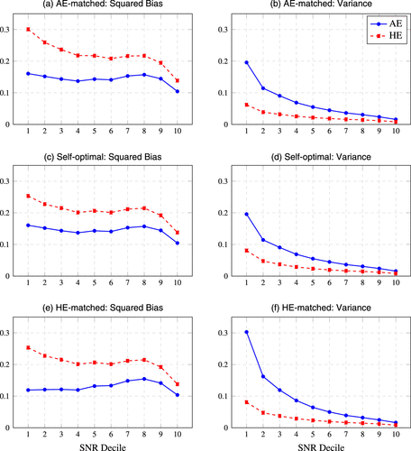
Notes. AE has lower bias, whereas HE has lower variance, across all regimes. AE outperforms HE in high-SNR settings because the variance gap closes faster than the bias gap as SNR increases.
The pattern is clean. AE has lower bias and HE has lower variance across all three regimes, with both gaps widest at low SNR and narrowing as signal strengthens. The variance gap closes faster, making AE the more likely winner as SNR increases. The results confirm the theory: honesty buys stability at the cost of fit, which can hurt accuracy when signal is strong.
Figure 7 further decomposes these quantities for the self-optimal regime. Squared bias is the sum of squared approximation bias, squared estimation bias, and their interaction. Variance is the sum of target coupling, noise overlap, and target-estimation spillover.
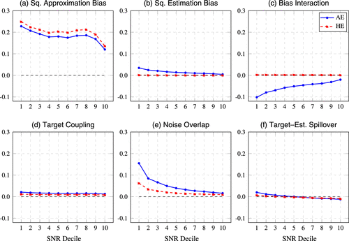
Note. Squared bias is dominated by approximation bias, whereas variance is dominated by noise overlap.
On the bias side, approximation bias dominates, and AE reduces it as theory predicts. Estimation bias is small for AE and zero for HE. Interestingly, the bias interaction for AE is negative: estimation bias actually reduces overall bias because the two components tend to have opposite signs. This is consistent with the stylized example in Section 3.2, where AE has negative approximation bias and positive estimation bias.
On the variance side, noise overlap accounts for most of the gap, and HE reduces it as theory predicts. Theory also predicts higher target coupling for HE at high SNR, but we do not observe it, suggesting the SNR threshold for that is too high to be practically relevant. Target-estimation spillover is generally closer to zero for HE, consistent with HE weakening the link between split selection and effect estimation.7
5. Discussion and Broader Implications
Honesty is widely treated as a conservative default in causal forests: it is built into common software, frequently recommended, and often adopted without much deliberation. Our results challenge this convention. Honesty is not inherently desirable and often degrades performance when treatment effect heterogeneity is substantial and the data large enough. In our empirical study, defaulting to honesty can require up to 27% more training data to match the performance of forests trained without it.
These findings have immediate implications for applied workflows that use causal forests for individual-level targeting, personalization, and prioritization.
Treat honesty as a hyperparameter. For the goal studied here—accurate CATE prediction at the individual level—there is little justification for adopting HE reflexively. Practitioners should treat honesty as a modeling choice, just like other complexity choices such as tree depth.
Adaptive estimation is a more sensible default. Most software packages default to honest estimation, but our results suggest the opposite default is more defensible. AE outperforms HE in most settings. In the cases where HE might seem preferable—when SNR is low and overfitting is a concern—the signal may be too weak for causal forests to reliably model heterogeneity at all. We return to this point below.
Choosing honesty often implies greater data requirements. When experiments are costly or samples are limited, the possibility that honesty may demand substantially more data to reach a given level of CATE accuracy should be part of the design conversation.
In our empirical analysis, we defined SNR as a property of the data-generating process, but it is better understood as a sample-dependent quantity. More data make effect heterogeneity easier to model, increasing the effective SNR and reducing the regularization benefit of honesty. AE tends to gain an advantage as sample size grows, but with sufficiently large samples both approaches perform well and practical differences diminish. Online Appendix H traces this progression empirically, showing the SNR-based insight holds even at hundreds of thousands of observations.
Honesty may still be preferable when the goal extends beyond predictive accuracy. Theoretical guarantees support HE for tasks like constructing confidence intervals or testing hypotheses, even at some cost to predictive accuracy. However, point estimation and uncertainty quantification do not need to rely on the same model. A practitioner could use an honest forest for testing or interval construction, and a separate adaptive forest for individual-level estimates used in targeting or personalization. The key is to match the estimation strategy to the objective rather than treating honesty as a universal default.
That said, causal forests may not even be the right tool in the first place. Before choosing between AE and HE, practitioners should assess whether causal forests are appropriate for their setting. Interestingly, the conditions that favor AE over HE may also be those where causal forests are most justified: high SNR implies substantial, detectable heterogeneity—precisely the regime where a flexible nonparametric learner gains an advantage over simpler alternatives. Conversely, when SNR is low and HE might seem preferable, the signal may be too weak for causal forests to reliably model heterogeneity at all. Indeed, in our empirical analysis, we find that the data sets where neither AE nor HE passes the heterogeneity test cluster heavily in low-SNR regimes. This suggests that when the signal is weak, the choice between AE and HE may matter less than the choice of whether to use causal forests at all.
The tension we study applies whenever the model structure is chosen using the same data later used for estimation—whether in tree-based methods, variable selection procedures, or ensemble learners. Separating selection from estimation reduces overfitting but limits flexibility to capture heterogeneity, and whether that trade-off is desirable depends on signal strength, sample size, and the analysis objective. Online Appendix G illustrates the same tension using adaptive and honest Lasso implementations on the ACIC data sets. At the same time, the specific decomposition components we analyze are closely tied to recursive partitioning methods and would likely manifest differently in other estimators. Systematically characterizing analogous components across CATE estimators is an interesting avenue for future research.
This paper highlights a distinction that is central to causal machine learning: the separation between approximation error and estimation error. In our setting, approximation error arises because the object we estimate—the SPATE associated with a leaf—is only an approximation to the individual-level CATE. Estimation error arises from sampling variability and selection bias in estimating those leaf-level effects. Honesty shifts the balance between these two sources of error.
A similar structural tension appears throughout causal inference. The statistical target—what can be identified from data, such as a conditional difference in means—need not equal the causal target, such as the CATE. In the presence of confounding, this mismatch is a form of approximation error: the estimable quantity does not equal the quantity of interest.
Identification assumptions formalize when this gap disappears. When they hold, approximation error vanishes, but finite-sample considerations remain. Choices that reduce approximation error, such as stronger identification strategies, can increase estimation error. A method that aggressively corrects for confounding bias may substantially increase variance, resulting in larger prediction error. The same tension appears when comparing randomized experiments to large observational data sets: experiments eliminate approximation error due to confounding, whereas observational data reduces estimation error through scale (Fernández-Loría and Provost 2025). Aligning the statistical and causal targets is ultimately a choice about how to navigate the bias-variance trade-off, much like honesty is in our setting.
The broader lesson is that causal analysis often involves trade-offs between approximation and estimation error. Our contribution is to make this trade-off explicit in heterogeneous treatment effect estimation with forests. Honesty is not a universal safeguard but a design choice that shapes this trade-off. More generally, we hope this perspective encourages researchers to ask, for any design choice in causal machine learning: how does it shift the balance between approximation and estimation error, and under what conditions does that shift help or hurt?
The authors dedicate this work to the memory of Sriram Somanchi. Conversations with Sriram during a visit to Dagstuhl convinced us that these findings were worth pursuing as a paper. They also helped shape the early direction of our research. His intellectual generosity, warmth, and curiosity were an inspiration to us, and he is deeply missed. The authors thank Foster Provost for many insightful discussions and constructive feedback throughout the development of this work. We are grateful to our research assistant, Pauline (Pui Lam) Luk, for doing much of the heavy lifting in organizing and synthesizing the literature review.
1 The bias is upward for individuals with and downward for those with .
2 One way to achieve this is to partition the original training data once into disjoint splitting and estimation subsets, and then subsample separately from each subset when learning every tree. However, we do not recommend this design because it would likely amplify target coupling and noise overlap.
3 We use the implementation from EconML (Battocchi et al. 2019). Each forest consists of 100 trees trained on subsamples of half the training data. We set other hyperparameters that affect model complexity, such as maximum depth, to nonbinding values so that regularization is governed by the min_samples_leaf parameter.
4 Online Appendix D.5 details the implementation of the test. As an empirical check, its false-positive rate on the 200 ACIC data sets with no true heterogeneity is 1.5% for both AE and HE, below the nominal 5% level.
5 As a robustness check, we repeat the full procedure under five independent treatment randomizations. The empirical selector achieves lower and than both AE and HE in every run. The gains are significant for against HE in all five runs and against AE in four, and for against AE in all five runs and against HE in four.
6 Under this standardization, signal loss decomposes as .
7 Because target effects are estimated from a finite auxiliary sample, the estimated spillover is shifted downward and can be negative even when the population quantity is positive. Its sign alone is therefore not informative; see Online Appendix F.
References
- (2015) Machine learning methods for estimating heterogeneous causal effects. Preprint, submitted April 5, https://arxiv.org/abs/1504.01132v1.Google Scholar
- (2016a) Recursive partitioning for heterogeneous causal effects. Proc. Natl. Acad. Sci. USA 113(27):7353–7360.Crossref, Google Scholar
- (2016b) The econometrics of randomized experiments. Preprint, submitted July 3, https://arxiv.org/abs/1607.00698.Google Scholar
- (2019) Generalized random forests. Ann. Statist. 47(2):1148–1178.Crossref, Google Scholar
- (2019) EconML: A Python package for ML-based heterogeneous treatment effects estimation, version 0.x. https://github.com/py-why/EconML.Google Scholar
- (1984) Classification and Regression Trees (Wadsworth International Group, Belmont, CA).Google Scholar
- (2019) Automated versus do-it-yourself methods for causal inference: Lessons learned from a data analysis competition. Statist. Sci. 34(1):43–68.Crossref, Google Scholar
- (2025) Observational vs. experimental data when making automated decisions using machine learning. INFORMS J. Data Sci. 4(3):197–229.Link, Google Scholar
- (2009) The Elements of Statistical Learning: Data Mining, Inference, and Prediction, 2nd ed. (Springer, New York).Crossref, Google Scholar
- (2025) Statistical inference for heterogeneous treatment effects discovered by generic machine learning in randomized experiments. J. Bus. Econom. Statist. 43(1):256–268.Crossref, Google Scholar
- (2021) Sharp analysis of a simple model for random forests. Banerjee A, Fukumizu K, eds. Proc. 24th Internat. Conf. Artificial Intelligence Statist., Proceedings of Machine Learning Research, vol. 130 (PMLR, New York), 757–765.Google Scholar
- (2016) On the asymptotics of random forests. J. Multivariate Anal. 146:72–83.Crossref, Google Scholar
- (2018) Estimation and inference of heterogeneous treatment effects using random forests. J. Amer. Statist. Assoc. 113(523):1228–1242.Crossref, Google Scholar
Yanfang Hou is a PhD student in information systems at HKUST Business School. Her research combines machine learning and causal inference to support data-driven decision making in business.
Carlos Fernández-Loría is an assistant professor of information systems at HKUST Business School. His research studies how predictive modeling and causal inference can inform decisions about whom to target with different interventions, with applications in recommendations, referrals, advertising, and payment compliance. He received his PhD from NYU Stern and is a coauthor of the forthcoming second edition of Data Science for Business.