
The Unintended Consequence of Land Finance: Evidence from Corporate Tax Avoidance
Abstract
Using a large sample of unlisted industrial firms in China, we find that a decrease in local governments’ land transfer revenues leads to lower tax avoidance by firms within their jurisdiction. Our cross-sectional variation tests suggest that the tax-avoidance-reduction effect is stronger in cities with higher land finance dependence and government intervention, as well as where the political leaders have stronger promotion incentives. However, the effect is moderated for politically connected firms. Further analysis reveals that intensified tax enforcement is the mechanism through which land transfer revenue losses result in decreased tax avoidance. Our study offers novel evidence on a previously underexplored determinant of corporate tax avoidance through the lens of land finance.
This paper was accepted by Gustavo Manso, finance.
Funding: The authors acknowledge financial support from the National Natural Science Foundation of China [Grants 72002105, 71972089 and 72132002]. T. Chen is grateful for the financial support from the Singapore Ministry of Education Academic Research Fund [Grant 2015-T2-1-118, RG166/18] and the Natural Science Foundation of Guangdong Province, China [Grants 2018A03031043 and 2019A1515011635]. C. (C.) Zeng acknowledges the start-up research fund from the Hong Kong Polytechnic University [Grant A0035237].
Supplemental Material: Data and the online appendix are available at https://doi.org/10.1287/mnsc.2021.4191.
1. Introduction
Local governments in many countries, especially developing countries (India, Egypt, Turkey, South Africa, and China, among others), have typically relied on land-based fiscal revenue (e.g., land-sale proceeds, land-leasing rent, and land-as-collateral borrowing) to finance infrastructure projects and boost local economic growth (often referred to as land finance) (Peterson and Kaganova 2010).1 However, high reliance on land finance for economic development is risky, because land markets can be highly volatile, particularly in developing countries (for more details, see Section 2.1). Given the volatility of land-sale revenue, it would be interesting to find out how local governments might circumvent the fiscal constraint as a result of losses of revenue from land finance. Our paper seeks to answer this question by examining the impact of land finance on corporate taxation, another major source of local fiscal revenue.
The determinants of corporate tax avoidance behavior have been studied extensively in recent years. This stream of research has uncovered a broad spectrum of parties and factors that may affect a firm’s tax behavior, such as shareholders (Chen et al. 2010, Cheng et al. 2012), debt holders (Hasan et al. 2014), executives (Armstrong et al. 2012, Koester et al. 2016), financial analysts (Chen and Lin 2017), labor unions (Chyz et al. 2013), customers and suppliers (Cen et al. 2017, Naritomi 2019), auditors (McGuire et al. 2012), credit rating agencies (Chen et al. 2021a), the public (Mills et al. 2013), import competition (e.g., Chen et al. 2021b), and the political environment (Baloria and Klassen 2017). Yet relatively little is known about the role of local governments in corporate taxation, despite the fact that the state is de facto the largest minority shareholder in firms because of its tax claim on cash flows (Desai et al. 2007). In particular, to the best of our knowledge, no study has investigated the relationship between land financing and corporate tax behavior, although the former is a crucial source of urban infrastructure finance around the world.
We examine this question in China because, as the largest developing country in the world, China provides a typical example of how local governments rely on land-based revenues to fulfill their economic and social objectives. Since 1998, subprovincial officials have been assigned statutory rights to sell land and exclusively retain the revenues. Because local governments are not required to share the revenue so generated with the upper-level authorities, they have eagerly tapped this new source of financing, flooding the local coffers. According to data from the National Bureau of Statistics of China (NBS), whereas land transfer revenue was negligible initially, accounting for only 16.6% of the entire local general budgetary revenue in 2001, this percentage has grown dramatically, to nearly 67.6% in 2010. In contrast to the trend in land transfer revenue, the effective tax rates (ETRs) of Chinese firms have declined constantly, falling from 14% in 2004 to 11.7% in 2010, exhibiting a clear countercyclical pattern. The decline in ETRs can be considered a benefit that land finance brings to business entities. Intuitively, to the extent that local governments depend heavily on land transfer revenues rather than corporate taxes to fill their coffers, the tax enforcement against corporate tax avoidance is likely to be lax, allowing firms to make tax savings and reserve those savings for future development.
The role of land finance in corporate taxation is especially conspicuous in China. A salient feature of China’s governance structure is regional decentralization, in which the central government directly controls the key positions at the provincial level and grants each tier of subnational government the power to appoint key officials one level below it. In order to increase their odds of being promoted to a higher rank in the hierarchy of the Chinese Communist Party (CCP), local government officials have to demonstrate the achievements they have made during their tenure in office (e.g., Maskin et al. 2000 and Li and Zhou 2005). Because local officials face multiple tasks, they often choose to focus on tasks that are more measurable (Qian 2000, Xu 2011). Under this system, economic development is generally a prioritized and predominant factor affecting the promotion of local officials (Xu 2011). The promotion path creates incentives for local officials to engage in interjurisdictional tax competition through lax tax enforcement aimed at attracting capital inflows, especially foreign investment. On the other hand, tax collection has also been ranked as an important criterion for assessing local officials’ promotion prospects, because it constitutes a clear and tangible signal of the competence of local officials and allows them to enhance their capacity to finance public expenditures, which can quickly translate into increased aggregate demand and economic growth (e.g., Kung and Chen 2014 and Lü and Landry 2014).2
Land finance has the potential to alleviate the above-mentioned conflicting demands facing local officials. Local governments with budgetary slack, arising from land transfer revenues, are in an advantageous position when it comes to engaging in tax competition while at the same time being able to finance infrastructure investment and public services. Consequently, the local officials are less motivated to strengthen tax enforcement, leaving considerable room for firms to avoid tax. For instance, Esteller-Moré (2005) finds that regional governments have less incentive to collect tax, and therefore devote less effort to it, when they receive unconditional grants from the central government. By contrast, for local governments suffering a fiscal squeeze, it is reasonable to expect that the costs of a lenient tax policy would outweigh the benefits. This is because, to meet their commitments to finance public services, local governments may be forced to raise fiscal revenues through stricter tax enforcement. Taken together, the costs and benefits of tax enforcement vary according to the fiscal condition of the local government. We therefore hypothesize that firms operating in regions experiencing a decline in land transfer revenues will be associated with more stringent tax enforcement and therefore lower tax avoidance.
To test this conjecture, we carry out empirical analysis using a comprehensive sample of 223,227 unique unlisted firms. We focus exclusively on unlisted firms for the following reasons. First, the firms covered by the NBS database account for 85% of China’s industrial value added. The performance of the estimated models is likely to be enhanced when using a more representative sample. Second, compared with unlisted firms, Chinese listed firms are not evenly distributed, geographically. More important, the distribution of listed firms is proportional to the economic power of the province in which the firms are domiciled. For instance, according to statistics, the province with the largest number of listed firms is Guangdong, with 577 listed firms, accounting for 16.42% of the country’s total. By contrast, there are no listed firms in less developed provinces such as Guangxi, Qinghai, Shanxi, and Inner Mongolia. To the extent that land finance is highly correlated with the economic size of the region, focusing on a geographically unbalanced sample such as listed firms is likely to yield biased results. Finally, despite the fact that unlisted firms make a major contribution to economic growth worldwide, their tax avoidance behavior has been relatively neglected in the previous research. Therefore, our study seeks to fill this void in the literature.
To measure tax avoidance for unlisted firms, we follow Cai and Liu (2009) and calculate an imputed corporate profit based on the national income accounts, by deducting intermediate inputs from gross output. We then use the sensitivity of the reported accounting profit to the imputed profit to measure the level of tax avoidance (see Section 3 for more details). The intuition is straightforward. To the extent that both profit figures reflect a firm’s economic fundamentals, a positive relationship between them will be indicative of a low level of tax avoidance. Therefore, our empirical strategy is to test how a deterioration in the land finance, as a result of a decline in land transfer revenues, of local governments affects the sensitivity of the reported profits to the imputed profits.
Our prediction is confirmed by the empirical results. We find strong evidence that a land revenue decline is associated with fewer tax avoidance activities. The estimated effects of land finance have the predicted signs, as well as statistical and economic significance. This result is robust to alternative specifications and an alternative sample, as well as to controlling for year, industry, city, and industry-year fixed effects.
One may reasonably be concerned that our independent variable, loss of land revenue, could be endogenous as a result of possible omitted variable bias and measurement errors. To mitigate the potential endogeneity concerns, we perform difference-in-differences (DID) analyses by exploiting several exogenous shocks to local housing markets. Intuitively, an exogenous decrease in housing prices is expected to exaggerate local governments’ budget constraints, which would in turn lead to more stringent tax enforcement and less corporate tax avoidance. We first use the 2006 North Korean nuclear test as a negative shock to the house prices in the cities in northeastern China. The results show that, following the nuclear test, tax avoidance decreases significantly for firms in the shocked cities but remains largely unchanged for those in the matched nonshocked cities. Next, following previous research (e.g., Fink and Stratmann 2015, Zhu et al. 2016, and Ando et al. 2017), we utilize the Fukushima nuclear accident, which was triggered by the 2011 Tōhoku earthquake and tsunami in Japan, as an alternative negative shock to the housing markets of cities near nuclear plants in China. Again, we find a significant decrease in tax avoidance only for firms in the shocked cities. The results of these identification tests, taken together, lend support to our prediction that corporate tax avoidance decreases as local fiscal constraints become more severe.
Moreover, we provide cross-sectional variation evidence on the effect of land finance on tax avoidance. Evidence consistent with theoretical predictions that land finance will have a larger impact on tax avoidance in certain circumstances lessens the endogeneity concern (Rajan and Zingales 1988, Jiang 2017). First, our results show that the effect is augmented by local government dependence on land finance. This finding suggests that when land revenue forms a greater portion of the local government’s fiscal revenue, a decrease in land sales revenue triggers stronger tax collection enforcement, leading to a larger decline in firms’ tax avoidance activities. Next, we find that the effect of land finance on tax avoidance is more pronounced for firms in regions with a higher level of government intervention. This is consistent with the notion that when local governments are more able to intervene in the market, they are more likely to implement strict tax regulations in the face of a reduction in land sales revenue. Third, the effect of land finance on tax avoidance is moderated in firms that are politically connected. This is consistent with the conventional belief that political connections can shield the connected firms from unwanted political interference and/or unfavorable regulations (Zhang et al. 2016). In addition, as discussed earlier, the tax capacity is, to a large extent, affected by the incentives of local officials. Our results confirm this argument by showing that the impact of land finance on corporate tax avoidance is more pronounced when the local political leaders have stronger incentives to gain promotions.
We argue that land revenue decline leads to stricter local tax enforcement, which, in turn, results in less corporate tax avoidance. To provide direct evidence to support this argument, we follow prior literature (e.g., Mertens 2003 and Lin et al. 2018) and measure the changes in enforcement actions using three proxies: the growth rate of the number of local tax officers, the growth rate of local tax audits, and a regression-based proxy for tax enforcement effort. In line with our conjecture, we find evidence suggesting that land finance constraints are positively associated with these tax enforcement measures. Moreover, the impact of land finance constraints on corporate tax avoidance is more pronounced in regions with stronger tax enforcement. To further tease out the tax enforcement effect, we perform a placebo test in which we use firms that are not subject to the local tax enforcement as a placebo sample. We find that the impact of land revenue losses on tax avoidance is confined to firms whose corporate income taxes are levied by the local governments. Our evidence is consistent with tax avoidance behavior being restricted by stringent tax enforcement by local governments with budgetary constraints.
Our study contributes to the literature in several ways. First, we contribute to an emerging literature on corporate tax avoidance (see Hanlon and Heitzman (2010) for a review). Despite the surge in the number of tax avoidance studies over the past decade, most studies have focused on firm-level determinants, with little attention paid to the position of the government, especially local government. This is probably because the taxing government is just a minority shareholder in the traditional Scholes et al. (1992) framework (Hanlon and Heitzman 2010). Our study seeks to fill this void by investigating how local land finance affects tax enforcement and corporate tax avoidance. Additionally, unlike most prior studies that use samples of listed firms, our paper focuses on the tax avoidance behavior of unlisted firms, which are economically important but relatively understudied in the literature.
Second, our paper adds to the understanding of the real consequences of price movements in the land market. Using a land market collapse in Japan as an exogenous shock to bank lending, Gan (2007) documents that firms’ investment and market valuation are negatively affected by their top lender’s real estate exposure. Chaney et al. (2012) find that representative U.S. firms invest six cents in response to a one-dollar increase in their land collateral, whereas Wu et al. (2015) find that such a collateral channel does not exist in the Chinese market. In a recent study, Gu et al. (2019) find that positive house price shocks affect individual shirking behavior.3 Nevertheless, as far as we are aware, no study to date has investigated the impact of the land market on corporate tax behavior. Our study therefore contributes to this nexus of literature.
Last, but not least, our study contributes to the understanding of the role of local fiscal behavior in developing and transitional economies. Although land finance has generated a variety of risks and challenges, our findings show that it has also played a critical role in relieving the tax burden on industrial firms and oiling the wheels of entrepreneurial and business activities. Given the prevalence of land financing around the world, the outcomes of our study are not merely confined to the context of China but provide a lens through which policy makers may better evaluate and manage local public finance worldwide.
The rest of the paper proceeds as follows. Section 2 introduces institutional background pertaining to land finance. Section 3 describes the data and variables. Section 4 presents the findings of the main analysis and robustness checks. Section 5 discusses the results of the cross-sectional variation analyses and channel tests. Section 6 concludes.
2. Institutional Background
2.1. Land Finance Around the World
Land assets are an important ingredient of local government finance in most developing countries, primarily because land is often the most valuable asset on the balance sheets of local governments.4 Direct sales of land by local governments are the clearest example of the capitalizing of land value. In addition, there are other instruments used to convert public land rights to cash, such as land leasing or land-as-collateral borrowing. Peterson (2008) provides a number of examples in which revenues derived from land financing constitute a considerable portion of local fiscal revenues. For instance, the sale of an old municipal bus station and former government building site in Istanbul in 2007 generated revenue of $1.5 billion, whereas the total municipal capital spending in Istanbul in 2005 was only $994 million. In Beijing, the land-leasing contract value in 2009 was equal to 45% of the total fiscal revenue.
Land finance has attracted widespread criticism. For example, the rapid pace of land conversion from agricultural to urban use has put countries’ farmland under great pressure (Chau and Zhang 2011). More notably, as land-related revenues form a major component of land finance, local governments sell land to developers and pocket the value added to the land following development. As a consequence, land finance is often considered to lie at the core of the housing bubble and has received plenty of attention from the media, including the Financial Times and the Economist.5 On top of this, a major concern with land finance is the high volatility of urban land prices, which results in steep fluctuations in land revenue from year to year. Hong Kong is a good example. Hong Kong’s economy has been stunningly successful. A key feature of its economic model is that the government relies heavily on land sales or revenue, whereas the tax burdens for individuals and corporations are very low.6 During the period 1996–2000, Hong Kong raised, via land-leasing revenues, an amount equal to 130% of its expenditure on public works and 18% of its entire budget expenditure. Nevertheless, as a consequence of the Asian financial crisis, land prices and demand for land fell dramatically during 2001–2003. The loss of revenues from land financing contributed to considerable fiscal deficits that reached 30% of fiscal revenues at their peak (Peterson and Kaganova 2010).
2.2. Land Transfer Revenue in China
In China, urban land belongs to the state, whereas rural land is the property of the collective (Yang et al. 2017, Cheng and Chung 2018). The state maintains a monopoly on what is known as the “primary land market” in urban areas. The land use rights are transferred via allocation (reserved for state-owned enterprises (SOEs) or nonprofit organizations) and conveyance (reserved for commercial enterprises). State allocation is transacted at an “allocation price,” consisting of the expropriation cost of the land, stipulated land fees, and a government-set allocation fee. The land use rights obtained through conveyance can be further transferred in a “secondary land market.” Given that the conveyance fees are partly determined by the market, these fees are substantially higher than the allocation prices.
Since the 1994 tax reform, revenue assignment has gradually been recentralized, with expenditure assignment left largely unchanged. This has created a substantial fiscal gap at the local level (Nitikin et al. 2012). In 2008, for example, the local governments contributed more than 78% of total public expenditure while receiving less than 47% of total government revenue. The lack of revenue has seriously compromised local governments’ ability to carry out infrastructure improvements and prevented them from offering social services, which could have adverse impacts on political leaders’ promotion prospects—and even lead to political repercussions. As a result, the local governments have strong incentives to raise revenue through various means.
The land market offers the local governments such an opportunity. Given China’s socialist nature, the government does not allow ownership of land converted into urbanization purposes to fall into the hands of private individuals, according to a law passed at the 15th National Congress of the Communist Party of China in 1998. As a result, local governments are assigned de jure ownership of land in their jurisdiction, and private individuals have only a limited tenure of 70 years of land use rights (Lin and Ho 2005). More important, local governments can keep all the proceeds from the sale of land under their jurisdiction as “extra-budgetary revenue,” which is deemed an unexpected source of revenue, or windfall (Chen and Kung 2016). According to the China Land and Resources Statistical Yearbook 2018, land transfer revenue accounted for 15% of the combined central and local government revenue in that year, serving as the second-largest revenue source, behind tax revenue. Moreover, land-related revenue is making up an increasing proportion of local governments’ revenue. For example, land-related revenue’s share of total local government revenue was less than 10% prior to 2000 but had increased dramatically to more than 20% by 2007. However, the volatility of the urban land market and the limited supply of land have prevented land-based revenues from forming a stable and sustainable source. Any significant decrease in land transfer revenues will inevitably put local governments under serious fiscal pressure, forcing them to tighten their tax enforcement so as to generate revenues from other sources.
3. Data, Sample, and Variables
3.1. Measurement of Tax Avoidance
A conventional measure of tax avoidance is the book-tax difference (Hanlon 2005, Blaylock et al. 2012). However, because book incomes are usually unavailable for unlisted firms, we cannot use this approach in our study. On top of this, Mills and Newberry (2001) suggest that book-tax differences are less informative about tax positions for private firms, because private firms are more likely to make book and tax conform to one another, which reduces the size of the book-tax differences for a given tax position. Another frequently used tax avoidance measure is generally accepted accounting principles (GAAP) ETR, which is computed as tax liability divided by pretax profits. Nevertheless, the ETR is likely to be noisy in our context for the following reasons. First, there are a large number of unlisted firms in our sample that report either missing or negative pretax income, making the GAAP ETR difficult to interpret. To mitigate this issue, some recent studies use cash flow as the denominator (i.e., cash ETR). However, the cash flow information is unavailable for our unlisted firms. Second, as pointed out by Hanlon and Heitzman (2010), because private firms are likely to achieve most of their avoidance of explicit taxes by reporting lower accounting earnings as well as lower taxable income, this type of tax avoidance would not be captured by the typical ETR measures.
Given these considerations, we follow Cai and Liu (2009) and use the association between the imputed profit and the true accounting profit to measure the degree of tax avoidance. Simply using the difference between these amounts to proxy for tax avoidance would not be appropriate because the two figures can legitimately differ from each other as a result of accounting standards. However, for our purposes, we only need to look at whether the two profit numbers are positively correlated, because both reflect a firm’s economic fundamentals. In other words, a strongly positive correlation between the imputed profit and the reported accounting profit would indicate a low level of tax avoidance. The NBS database covers information on inputs and outputs for every sample firm, which allows us to compute the imputed profit (PRO) defined according to the national income accounting system as follows:
3.2. Measurement of Land Transfer Revenue Losses
The term LAND is defined as state-owned land transfer revenues divided by local gross domestic product (GDP); ΔLANDloss is the change in the state-owned land transfer revenues, which equals LAND in year t − 1 minus LAND in year t, divided by LAND in year t − 1. A higher value of ΔLANDloss stands for a greater decline in land sales revenue for the local government in year t.
3.3. Control Variables
Following Cai and Liu (2009), the control variables used in the main analysis include the following: FINANCE, defined as a firm’s financial charges divided by its total assets, which is a proxy for the firm’s access to credit markets; RSALE, defined as a firm’s sales divided by its total output; SIZE, defined as the natural logarithm of the number of employees; and SOE, which equals 1 if the firm is a state-owned enterprise and 0 otherwise. We also include city, industry, and year fixed effects, or industry-year fixed effects. The standard errors are clustered at the city level to correct for within-city correlation. All continuous variables are winsorized at the 0.5% and 99.5% levels. The variable definitions are provided in Appendix A.
3.4. Sample and Data
The primary data source used in our study is the NBS, which provides annual survey data for all industrial firms with annual sales of more than RMB 5 million (approximately USD 780,000). Those firms account for more than 85% of China’s industrial value added. The firm-level information includes industry code, ownership, region code, value added, sales revenue, and various tax payments, among other items. Currently, the NBS database provides the most comprehensive coverage for Chinese unlisted firms, with approximately 200,000 firms included each year.7 The information reported to the NBS should be highly reliable, because the NBS implements a standard procedure for calculating the national income accounts and double-checks the information in a strict manner. Also, firms do not have any incentives to misreport their information to the NBS, because such information cannot be used against them by other government agencies such as the tax authorities (Cai and Liu 2009).
The city-level information is manually collected from the China City Statistics Yearbook, which covers information on government revenue and expenditure for cities at and above the prefecture level. Information on land transfer revenue is derived from the China Land and Resources Statistics Yearbook. Finally, personal information on government officials is obtained from the China Stock Market Accounting Research (CSMAR) database.
We use data from 1999 to 2012, spanning 34 provinces or province-equivalent municipal cities and 289 prefecture-level cities. We combine the above-mentioned databases and drop four types of observations, following Cai and Liu (2009): (1) observations with missing values for key variables—namely, total assets, number of employees, industrial output, profit, and depreciation expense; (2) observations with a negative value for total assets, intermediate input, or total fixed assets; (3) observations with total assets less than net fixed assets, or with accumulated depreciation less than current depreciation; and (4) observations for which one of the following is true: the value of fixed assets is below RMB 10 million, the value of total assets is below RMB 10 million, or the number of employees is less than 30. This procedure yields a final sample of 687,908 observations, representing 223,227 unique firms.
4. Empirical Results
4.1. Summary Statistics
Summary statistics for the variables used in the regressions are reported in Table 1. The mean of the reported profit is 0.0885, with a standard deviation of 0.1672, whereas the mean of the imputed profit is 0.1465, with a standard deviation of 0.3817. These figures are highly consistent with those reported in Cai and Liu (2009).8 The difference between the two profit measures may reflect the differences between the accounting system and the national income accounting system. Moreover, the mean of ΔLANDloss is −0.3945, suggesting that, on average, the local governments profit from transferring state-owned lands during our sample period. However, the median of ΔLANDloss is positive, suggesting the presence of a loss of revenue from land transfers. The measure also has a large standard deviation, showing that there is substantial heterogeneity in land-financing activities and land price growth across cities (e.g., Deng et al. 2012 and Wu et al. 2014). In addition, the summary statistics for the control variables are consistent with those reported in Cai and Liu (2009).
|

Table 1. Summary Statistics
| Variable | Mean | Std. dev. | 25th %ile | Median | 75th %ile |
|---|---|---|---|---|---|
| (1) | (2) | (3) | (4) | (5) | |
| RPRO | 0.0885 | 0.1672 | 0.0035 | 0.0362 | 0.1126 |
| PRO | 0.1465 | 0.3817 | −0.0293 | 0.0729 | 0.2427 |
| FINANCE | 0.0155 | 0.0187 | 0.0022 | 0.0107 | 0.0229 |
| SIZE | 5.6023 | 1.0425 | 4.9053 | 5.5607 | 6.2186 |
| RSALE | 1.0138 | 0.3143 | 0.9308 | 0.9948 | 1.0232 |
| SOE | 0.1679 | 0.3738 | 0 | 0 | 0 |
| LAND | 0.0420 | 0.0327 | 0.0174 | 0.0365 | 0.0586 |
| ΔLANDloss | −0.3945 | 1.7234 | −0.4576 | 0.0161 | 0.2917 |
| D_ΔLANDloss | 0.7229 | 0.4476 | 0 | 1 | 1 |
| D_ FISPRO | 0.4998 | 0.5000 | 0 | 0 | 1 |
| High_GI | 0.5132 | 0.4998 | 0 | 1 | 1 |
| PC | 0.0320 | 0.1759 | 0 | 0 | 0 |
| D_SWAGE | 0.6138 | 0.4869 | 0 | 1 | 1 |
| D_CHANGE | 0.7876 | 0.4090 | 1 | 1 | 1 |
| D_Before2002 | 0.7913 | 0.4064 | 1 | 1 | 1 |
| D_TENURE_SAT | 0.3669 | 0.4820 | 0 | 0 | 1 |
| Treat_N | 0.5015 | 0.5000 | 0 | 1 | 1 |
| Post_N | 0.5745 | 0.4944 | 0 | 1 | 1 |
| Treat_FN | 0.5171 | 0.4997 | 0 | 1 | 1 |
| Post_FN | 0.6453 | 0.4784 | 0 | 1 | 1 |
| OFFICER_G | 0.0167 | 0.2450 | −0.0165 | 0.0040 | 0.0278 |
| TAX AUDIT_G | 0.2581 | 1.4795 | −0.3130 | −0.0424 | 0.3355 |
| TEE | 0.0001 | 0.0066 | −0.0032 | −0.0000 | 0.0029 |
| L.ΔLANDloss_P | −0.6181 | 2.4846 | −0.6816 | −0.2653 | 0.0496 |
| INFLATION | 0.0022 | 0.0301 | −0.0195 | 0.0083 | 0.0255 |
| ln(GDP) | 17.9371 | 1.0865 | 17.2852 | 18.0514 | 18.6791 |
| GDP_G | 0.1442 | 0.0435 | 0.1162 | 0.1472 | 0.1746 |
| IND1 | 12.7403 | 6.5163 | 8.90 | 12.75 | 16.60 |
| IND2 | 47.1257 | 8.0432 | 43.10 | 48.70 | 52.80 |
| UNEMPLOYMENT | 3.7284 | 0.6884 | 3.40 | 3.80 | 4.17 |
Notes. This table reports the summary statistics for variables used in the main analyses. Variable definitions are provided in Appendix A. %ile, percentile.
4.2. Baseline Regression Results
To assess the impact of local land finance on corporate tax avoidance, we estimate the following regression model:
Table 2 presents the ordinary least squares (OLS) regression results. In columns (1)–(5), the land transfer revenue loss is measured as ΔLANDloss, whereas in columns (6) and (7), we use an alternative proxy (D_ΔLANDloss), a dummy variable that equals 1 if ΔLANDloss is above the sample mean and 0 otherwise. In column (1), we only include the imputed profit and city dummy variables in the regression. The coefficient on PRO is positive and statistically significant at the 1% level. In column (2), we add all variables shown in Equation (2) except for the land transfer revenue variable and its interaction with the imputed profit. The coefficient on PRO remains positive but insignificant. In column (3), we only consider the impact of land finance on tax avoidance, without controlling for other variables, except the city, year, and industry fixed effects. The coefficient on the interaction term PRO × ΔLANDloss is positive and statistically significant. This result is not sensitive to adding in the control variables, as shown in column (4), nor to replacing the city, year, and industry fixed effects with industry-year and city fixed effects, as seen in column (5). These results consistently show that land transfer revenue losses are negatively associated with corporate tax avoidance.
|
Table 2. Baseline Regressions
| Variable | DV = RPRO | ||||||
|---|---|---|---|---|---|---|---|
| (1) | (2) | (3) | (4) | (5) | (6) | (7) | |
| PRO | 0.1767*** | −0.0024 | 0.1689*** | 0.0005 | −0.0013 | −0.0175 | −0.0173 |
| (20.53) | (−0.14) | (20.85) | (0.03) | (−0.08) | (−0.89) | (−0.88) | |
| ΔLANDloss | −0.0010* | −0.0006 | −0.0005 | ||||
| (−1.78) | (−1.26) | (−1.22) | |||||
| PRO × ΔLANDloss | 0.0114*** | 0.0072*** | 0.0063*** | ||||
| (7.06) | (4.87) | (4.42) | |||||
| D_ΔLANDloss | −0.0026 | −0.0022 | |||||
| (−0.95) | (−0.86) | ||||||
| PRO × D_ΔLANDloss | 0.0217** | 0.0193** | |||||
| (2.42) | (2.17) | ||||||
| PRO × FINANCE | 1.5334*** | 1.5399*** | 1.5097*** | 1.5302*** | 1.5009*** | ||
| (8.44) | (8.51) | (8.50) | (8.54) | (8.52) | |||
| PRO × SIZE | −0.0069** | −0.0071*** | −0.0071*** | −0.0072*** | −0.0072*** | ||
| (−2.54) | (−2.64) | (−2.65) | (−2.69) | (−2.70) | |||
| PRO × RSALE | 0.2389*** | 0.2380*** | 0.2384*** | 0.2381*** | 0.2386*** | ||
| (17.53) | (17.45) | (17.44) | (17.56) | (17.55) | |||
| PRO × SOE | −0.0135 | −0.0087 | −0.0081 | −0.0093 | −0.0086 | ||
| (−1.43) | (−0.92) | (−0.88) | (−1.03) | (−0.97) | |||
| FINANCE | −0.2450** | −0.2463** | −0.2343** | −0.2454** | −0.2334** | ||
| (−2.55) | (−2.57) | (−2.46) | (−2.56) | (−2.45) | |||
| SIZE | −0.0003 | −0.0002 | −0.0003 | −0.0002 | −0.0003 | ||
| (−0.37) | (−0.30) | (−0.35) | (−0.30) | (−0.34) | |||
| RSALE | 0.1001*** | 0.0991*** | 0.0968*** | 0.0992*** | 0.0969*** | ||
| (17.82) | (17.83) | (17.85) | (17.89) | (17.93) | |||
| SOE | −0.0426*** | −0.0430*** | −0.0417*** | −0.0431*** | −0.0417*** | ||
| (−22.00) | (−22.06) | (−21.94) | (−22.07) | (−21.94) | |||
| Constant | 0.0626*** | −0.0514*** | −0.0055 | −0.0508*** | −0.0446*** | −0.0485*** | −0.0425*** |
| (49.62) | (−5.63) | (−0.77) | (−5.56) | (−4.61) | (−5.22) | (−4.31) | |
| Industry FE | No | Yes | Yes | Yes | No | Yes | No |
| Year FE | No | Yes | Yes | Yes | No | Yes | No |
| Ind × Year FE | No | No | No | No | Yes | No | Yes |
| City FE | Yes | Yes | Yes | Yes | Yes | Yes | Yes |
| Observations | 687,908 | 687,908 | 687,908 | 687,908 | 687,908 | 687,908 | 687,908 |
| Adj. R2 | 0.2701 | 0.3743 | 0.3318 | 0.3747 | 0.3810 | 0.3747 | 0.3810 |
Notes. This table presents the baseline regression results under different specifications. Columns (1)–(5) present the results using ΔLANDloss as the independent variable, whereas columns (6) and (7) use D_ΔLANDloss as the independent variable. Reported in parentheses are T-statistics based on robust standard errors clustered at the city level. Variable definitions are provided in Appendix A. DV, dependent variable; FE, fixed effects.
***, **, and * represent significance at the 0.01, 0.05, and 0.10 levels, respectively.
In columns (6) and (7), we replace ΔLANDloss with D_ΔLANDloss. The coefficients on the interaction terms are still significantly positive. The economic significance is also meaningful. Take, for example, the results in column (6). On average, the responsiveness of the reported profit to the imputed profit, for firms in cities with larger land transfer revenue losses, increases by 0.0217 more than for firms in cities with lower land transfer revenue losses. This translates into a 2.5% decrease in corporate tax avoidance within their jurisdictions in response to a one-standard-deviation increase in land transfer revenue losses for the local governments, for representative firms with an average imputed profit of the sample.
The results on the control variables are mostly consistent with our expectations. A firm’s incentive to avoid tax should be negatively associated with its financial performance. This is supported by the significantly positive coefficient on the interaction between sales and imputed profit. Moreover, the coefficients on the interaction between firm size and imputed profit are significantly negative, suggesting that larger firms are more likely to avoid corporate tax.
4.3. Identification Tests
Although the OLS regression results support our hypothesis, they should be interpreted with caution. There might be omitted variables in our model specification, which could result in an endogeneity problem if these variables are correlated with both dependent and independent variables in our model. For instance, booming local economic conditions may affect land sales revenue and tax enforcement intensity simultaneously. Moreover, the imputed profit and the land finance variables in our model are likely to be measured with error, which would make the OLS estimates biased and inconsistent. To circumvent these concerns, we adopt the following identification approaches.
4.3.1. The North Korean Nuclear Test.
We first examine the impact of the 2006 North Korean nuclear test on the corporate tax avoidance of Chinese firms using a DID estimation.9 Because the test took place only approximately 100 kilometers (62 miles) from the China–North Korea border, tremors from the explosion spread into northeastern China, raising considerable anxieties about possible injuries to citizens as well as long-run contamination of the air, water, and soil. As a consequence, the test had an adverse impact on housing markets in northeastern China, especially in cities near to the China–North Korea border. In Panel A of Table 3, we define cities in the three northeastern provinces (Jilin, Heilongjiang, and Liaoning) as our treatment group, and we select the control group with two procedures. First, we employ the nearest matching in terms of city-level characteristics, including TRANSFER (percentage of total budgetary spending in a province funded by intergovernmental transfer), INCOME_D (revenue share of subprovincial governments in a province), EXPENSE_D (expenditure share of subprovincial governments in a province), TENURE (a provincial party secretary’s accumulated time in office by the end of that year), IND2 (the secondary industry ratio), IND3 (the tertiary industry ratio), ln(GDP_Per) (the logarithm of GDP per capita), GDP_G (the growth rate of GDP), INVEST (the proportion of local investment), and DEFICIT (the local government expenditures minus revenues, then divided by local revenues), measured in the year 2006. Next, for each firm in the treatment city, we select a firm from the control city using the nearest matching (without replacement) based on firm covariates that are used in the main regression. Post_N is a dummy variable that equals 1 for the years 2007 and 2008 and 0 for the years 2005 and 2006. In line with our expectation, we find that the tax avoidance of treatment group firms significantly declines following the nuclear test. However, firms in the control group do not experience a significant change in tax avoidance. As shown in columns (5) and (6), the impact of the nuclear test on tax avoidance is significantly different between the treatment and control groups.10
|
Table 3. North Korean Nuclear Test
| Panel A: Effects of North Korean nuclear test on tax avoidance | ||||||
|---|---|---|---|---|---|---|
| Variable | DV = RPRO | |||||
| Subsamples | Full sample | |||||
| Treatment | Control | Treatment | Control | |||
| (1) | (2) | (3) | (4) | (5) | (6) | |
| PRO | −0.0087 | 0.1046*** | −0.0085 | 0.1044*** | 0.0688*** | 0.0694*** |
| (−0.27) | (3.49) | (−0.27) | (3.49) | (3.05) | (3.09) | |
| PRO × Post_N | 0.0488*** | −0.0007 | 0.0465*** | −0.0037 | 0.0025 | −0.0016 |
| (5.54) | (−0.09) | (5.20) | (−0.47) | (0.33) | (−0.21) | |
| Post_N | −0.0416 | −0.0033 | −0.0295 | |||
| (−1.07) | (−0.17) | (−1.24) | ||||
| PRO × Treat_N× Post_N | 0.0438*** | 0.0463*** | ||||
| (3.72) | (3.95) | |||||
| PRO × Treat_N, Post_N × Treat_N | CONTROLLED | |||||
| Other control variables | Yes | Yes | Yes | Yes | Yes | Yes |
| Year FE | Yes | Yes | No | No | Yes | No |
| Industry FE | Yes | Yes | No | No | Yes | No |
| Ind × Year FE | No | No | Yes | Yes | No | Yes |
| City FE | Yes | Yes | Yes | Yes | Yes | Yes |
| Observations | 16,380 | 16,284 | 16,380 | 16,284 | 32,664 | 32,664 |
| Adj. R2 | 0.3043 | 0.3876 | 0.3126 | 0.3887 | 0.3452 | 0.3485 |
| Panel B: Parallel trend tests of North Korean nuclear test | ||||||
| Variable | DV = RPRO | |||||
| (1) | (2) | |||||
| PRO | 0.0878*** | 0.0860*** | ||||
| (3.79) | (3.72) | |||||
| PRO×Treat_N× Year_2006 | 0.0071 | 0.0059 | ||||
| (0.52) | (0.44) | |||||
| PRO × Treat_N× Year_2007 | 0.0771*** | 0.0779*** | ||||
| (5.24) | (5.29) | |||||
| PRO × Treat_N × Year_2008 | 0.0278* | 0.0307* | ||||
| (1.65) | (1.83) | |||||
| Other control variables | Yes | Yes | ||||
| Year FE | Yes | No | ||||
| Industry FE | Yes | No | ||||
| Ind × Year FE | No | Yes | ||||
| City FE | Yes | Yes | ||||
| Observations | 32,664 | 32,664 | ||||
| Adj. R2 | 0.3464 | 0.3495 | ||||
Notes. This table presents the results using the North Korean nuclear test that occurred on October 9, 2006, as an exogenous shock to land transfer revenue. Panel A examines the effect of the nuclear test on corporate tax avoidance using a matched sample. We define firms located in northeast China (Jilin Province, Heilongjiang Province, and Liaoning Province) as the treatment group, and we select a control group using a two-step matching process according to city- and firm-level characteristics. Post_N equals 1 for the years 2007 and 2008 and 0 for the years 2005 and 2006. Panel B presents the parallel trend results. The indicator variables Year_2006, Year_2007, Year_2008 flag the years 2006, 2007, and 2008, respectively. Reported in parentheses are T-statistics based on robust standard errors clustered at the firm level. Variable definitions are provided in Appendix A. DV, dependent variable; FE, fixed effects.
*** and * represent significance at the 0.01 and 0.10 levels, respectively.
To verify the parallel trend assumption, we include three indicators: Year_2006 (a dummy variable that equals 1 for the year 2006), Year_2007 (a dummy variable that equals 1 for the year 2007), and Year_2008 (a dummy variable that equals 1 for the year 2008), and we interact them with PRO × Treat_N. The results are reported in Panel B of Table 3. In line with the parallel trend assumption, the coefficient on the triple interaction term PRO × Treat_N× Year_2006 is insignificant, but the coefficients on both PRO × Treat_N× Year_2007 and PRO × Treat_N× Year_2008 are significantly positive.
To further validate that the nuclear test provides an appropriate setting for a DID analysis, we conduct a placebo test by randomly choosing a group of pseudo-treatment and pseudo-control firms. We repeat this procedure 1,000 times. Figure 1(a) illustrates the results. The mean coefficient estimated in the placebo test (−0.0003) is substantially smaller than the magnitude of the actual coefficient estimated from the main test (0.0438), suggesting that the observed impact of the nuclear test on corporate tax avoidance is not spurious. In addition, we plot the average logarithms of local land prices and GDP for the treatment and control cities surrounding the nuclear test. Figure A1(a) in the online appendix depicts the trends in local land prices and shows that the two lines exhibit a parallel trend before the nuclear test. However, following the test, the line representing the treatment group experiences a downward trend. When it comes to Figure A1(b) (in the online appendix), which illustrates the trends in local GDP, the two lines maintain a similar pattern in both pre- and posttest periods. This suggests that the impact of the nuclear test on tax avoidance is unlikely to be driven by changes in local economic fundamentals.
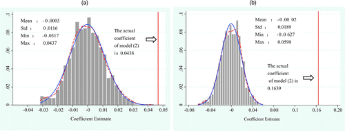
Notes. These figures show histograms of the coefficients on PRO × Treat × Post from bootstrap simulations of the model in Table 2. For each iteration, we draw a random sample of firms (the number is the same as the number of actual treated firms under each shock) as the “pseudo treatment group,” and the rest of the pool are used as the “pseudo control group.” On the basis of these “pseudo” treatment and control groups, we reestimate column (4) of Table 2 and save the coefficients on PRO × Treat × Post. We repeat this procedure 1,000 times. Figures (a) and (b) report the distribution of the coefficients for the North Korean nuclear test and Fukushima nuclear accident, respectively.
4.3.2. The Fukushima Nuclear Accident.
The Fukushima nuclear accident (FNA) was triggered by the 2011 Tōhoku earthquake and tsunami off the coast of Japan. It was the most severe nuclear accident to have happened since the Chernobyl disaster of 1986 and caused not only massive damage to the Japanese economy but also public concerns in many other countries, and especially negative effects to housing markets located near nuclear power plants (see, e.g., Bauer et al. (2017) for Germany, Fink and Stratmann (2015) for the United States, Zhu et al. (2016) for China, and Ando et al. (2017) for Sweden, among others). In particular, Zhu et al. (2016) find that the accident had a varied impact on land markets in China. More precisely, land prices within 40 km of nuclear power plants in China dropped by approximately 18% one month after the accident. However, the authors find no significantly negative impact beyond that distance.
Following this line of research, we utilize the accident as a negative shock to Chinese land markets and use a DID regression to estimate the impact of the shock on corporate tax avoidance. Specifically, the treatment group consists of cities within 40 km of any nuclear plant in China, whereas the control group comprises cities that are 40–200 km away from nuclear plants but from the provinces adjacent to the treated cities. We obtain the data on nuclear power plants in China from the World Nuclear Association, an international organization with members from various nuclear-related industries. To rule out confounding effects associated with housing purchase restriction polices (HPRP), we exclude cities that adopted HPRP in 2011 from our sample. Moreover, because the FNA had a short-run effect on land markets (Zhu et al. 2016), we focus on a narrow window (i.e., two years before and two years after the accident). We define a dummy variable, Post_FN, that equals 1 for the years 2011 and 2012 and 0 for the years 2009 and 2010.
Panel A of Table 4 shows that the coefficients on the interaction term PRO × Post_FN are significantly positive for the treatment group, suggesting a lower level of tax avoidance following the FNA. However, we do not find similar results for the control group. These findings reaffirm that deteriorating land revenue makes corporate tax avoidance less likely. To verify the parallel trend assumption, we include three indicators: Year_2010 (a dummy variable that equals 1 for the year 2010), Year_2011 (a dummy variable that equals 1 for the year 2011), and Year_2012 (a dummy variable that equals 1 for the year 2012), and we interact them with PRO × Treat_FN. The results reported in Panel B show that the parallel trend assumption indeed holds; that is, the coefficients on the triple interaction term PRO × Treat_FN × Year_2010 are insignificant, but the coefficients on both PRO × Treat_FN × Year_2011 and PRO × Treat_FN × Year_2012 are significantly positive.
|
Table 4. Fukushima Nuclear Accident
| Panel A: Effects of Fukushima nuclear accident on tax avoidance | ||||||
|---|---|---|---|---|---|---|
| Variable | DV = RPRO | |||||
| Subsamples | Full sample | |||||
| Treatment | Control | Treatment | Control | |||
| (1) | (2) | (3) | (4) | (5) | (6) | |
| PRO | −0.1099* | −0.0499 | −0.1213** | −0.0442 | −0.0781* | −0.0768* |
| (−1.90) | (−1.05) | (−2.07) | (−0.93) | (−1.95) | (−1.91) | |
| PRO×Post_FN | 0.1715*** | 0.0145 | 0.1774*** | 0.0102 | 0.0113 | 0.0108 |
| (9.43) | (1.29) | (9.76) | (0.89) | (1.01) | (0.95) | |
| Post_FN | −0.1578*** | −0.1099** | −0.0848** | |||
| (−3.69) | (−2.08) | (−2.27) | ||||
| PRO × Treat_FN × Post_FN | 0.1639*** | 0.1754*** | ||||
| (8.46) | (8.98) | |||||
| PRO × Treat_FN, Post_FN × Treat_FN | CONTROLLED | |||||
| Other control variables | Yes | Yes | Yes | Yes | Yes | Yes |
| Year FE | Yes | Yes | No | No | Yes | No |
| Industry FE | Yes | Yes | No | No | Yes | No |
| Ind × Year FE | No | No | Yes | Yes | No | Yes |
| City FE | Yes | Yes | Yes | Yes | Yes | Yes |
| Observations | 7,638 | 7,134 | 7,638 | 7,134 | 14,772 | 14,772 |
| Adj. R2 | 0.4534 | 0.2160 | 0.4623 | 0.2197 | 0.3257 | 0.3284 |
| Panel B: Parallel trend tests of Fukushima nuclear accident | ||||||
| Variable | DV = RPRO | |||||
| (1) | (2) | |||||
| PRO | −0.0944** | −0.0941** | ||||
| (−2.30) | (−2.29) | |||||
| PRO × Treat_FN × Year_2010 | 0.0343 | 0.0255 | ||||
| (1.23) | (0.93) | |||||
| PRO × Treat_FN× Year_2011 | 0.0943*** | 0.0911*** | ||||
| (3.31) | (3.19) | |||||
| PRO × Treat_FN × Year_2012 | 0.2189*** | 0.2311*** | ||||
| (10.03) | (10.44) | |||||
| Other control variables | Yes | Yes | ||||
| Year FE | Yes | No | ||||
| Industry FE | Yes | No | ||||
| Ind × Year FE | No | Yes | ||||
| City FE | Yes | Yes | ||||
| Observations | 14,772 | 14,772 | ||||
| Adj. R2 | 0.3306 | 0.3334 | ||||
Notes. This table presents the results using the 2011 Fukushima nuclear accident (FNA) as an exogenous shock to land transfer revenue. In Panel A, we concentrate our analysis on areas within a 200-kilometer radius of the power plants, and Treat_FN is a dummy variable that equals 1 for firms headquartered within 40 kilometers of a nuclear power plant and 0 for those headquartered within 40–200 kilometers. Post_FN equals 1 for the years 2011 and 2012 and 0 for the years 2009 and 2010. In Panel B, we present the parallel trend results. The indicator variables Year_2010, Year_2011, and Year_2012 flag the years 2010, 2011, and 2012, respectively. Reported in parentheses are T-statistics based on robust standard errors clustered at the firm level. Variable definitions are provided in Appendix A. DV, dependent variable; FE, fixed effects.
***, **, and * represent significance at the 0.01, 0.05, and 0.10 levels, respectively.
To further verify that the FNA provides an appropriate setting for our DID analysis, we conduct a placebo test by randomly choosing a group of pseudo-treatment and pseudo-control firms. We repeat this procedure 1,000 times. Figure 1(b) illustrates the results. The mean coefficient estimated in the placebo test (−0.0002) is substantially smaller than the magnitude of the actual coefficient estimated from the main test (0.1639), suggesting that the observed impact of the FNA on corporate tax avoidance is unlikely to be driven by chance. Again, we plot the average logarithms of local land prices and GDP for treatment and control cities surrounding the FNA. Figure A1 (c) in the online appendix illustrates the trends in land prices. The two lines trend closely in parallel in the years before the accident, whereas the line representing treatment firms begins to trend downward following the event. In a similar vein, we plot the trends of local GDP between the two groups in Figure A1(d) (in the Online Appendix). The two lines trend in parallel in both pre- and postevent periods, suggesting that local economic fundamentals were not affected by the FNA.11
4.4. Other Robustness Checks
4.4.1. An Alternative Explanation: Budgetary Pressure.
An alternative explanation for the relationship between land sales revenue losses and corporate tax avoidance is that local governments’ budgetary deficits in the previous year can lead to more aggressive land sales in the following year. As such, higher land transfer revenue in the current year could reflect an improvement in the local government’s budgetary pressure in the previous year. As such, the local governments have less incentive to intensify tax enforcement (Deng et al. 2012, Hsu et al. 2017). In this subsection, we assess the validity of this alternative explanation using multiple approaches.12
We begin by testing the impact of budgetary deficits on land supply and land revenue. We use two measures for land supply: LANDsupply (the logarithm of the total floor space sold by governments in each prefecture-level city in each year) and ΔLANDsupply (LANDsupply in year t minus LANDsupply in year t − 1). We also use two proxies for land sale revenue losses: ΔLANDloss (defined in Section 3.2) and D_Loss (= 1 if ΔLANDloss is above 0 and otherwise 0). A higher value of ΔLANDloss stands for a larger decline in land sales revenue for the local government in year t. The independent variable L.DEFICITbudget is the government budget deficit in the previous year, measured as the difference between budgetary expenditure and budgetary income in year t − 1, scaled by budgetary income in year t − 1. Following prior research (e.g., Deng et al. 2012 and Hsu et al. 2017), we control for the following variables: ln(Pop_Increase) (the logarithm of the population increase), ln(GDP_per_Increase) (the logarithm of the increase in GDP per capita), TENURE (the length of the prefectural party secretary’s term), TENURE_Square (the square of TENURE), IND2 (the secondary industry ratio), and IND3 (the tertiary industry ratio). We also control for year and city fixed effects and cluster standard errors at the city level.
The regression results are reported in Online Appendix R2. We find that although the budget deficit in the previous year is significantly positively associated with land supply, it is insignificantly associated with land transfer revenue. These results are largely consistent with those reported in table 7 of Hsu et al. (2017). It is conceivable that land sales revenue and land supply show different patterns because local governments may hoard land supply in order to gain higher land sales revenue later (Du and Peiser 2014). The insignificant relation between budget deficit and land sales revenue could help mitigate the concern that the relationship between local government land-sale finance and corporate tax avoidance is driven by the local government budget deficit.
To further rule out the possible confounding effects associated with the city-level determinants of land revenue losses, we use the residual of the land revenue losses (Residual ΔLANDloss), estimated from column (2) of Online Appendix R2, as the independent variable and repeat our main regression. Because Residual ΔLANDloss is orthogonal to the known determinants of land revenue losses, it measures the unexpected shocks to a city’s land sales revenue losses. A larger value of the residual corresponds to a greater loss in the land revenue. The results are reported in Panel A of Online Appendix R3. Our main findings continue to hold with this alternative independent variable.
Moreover, we reestimate our main regression model using a propensity-score-matched sample. The procedure involves the following steps: First, we partition the full sample into two groups based on the dummy variable D_Loss, which equals 1 if ΔLANDloss is above 0 and otherwise 0. Second, we derive the propensity scores from column (3) of Online Appendix R2 (i.e., the predicted value). We then implement nearest-neighbor matching for each treatment city by selecting a control city that has the closest propensity score in the same year. Next, for each firm in the treatment city, we select a firm in the control city (without replacement) that has the closest propensity score in terms of firm-level covariates that are used in the main regression.13 Finally, we repeat our main regression using the matched sample. This approach ensures that the treatment and control firms are largely indistinguishable for a set of city- and firm-level characteristics. This could greatly alleviate the confounding effects related to observable city and firm heterogeneities. Panel B of Online Appendix R3 presents the regression results using the matched sample. Our main inferences remain unchanged using this alternative sample.
4.4.2. Alternative Sample and Measures of Land Transfer Revenue Losses.
We carry out a robustness test using another restricted sample. In Online Appendix R4, we show the results of removing firms located in 4 municipalities (Beijing, Shanghai, Tianjin, and Chongqing) and 15 subprovincial cities (Guangzhou, Nanjing, Shenzhen, Wuhan, Shenyang, Xi’an, Chengdu, Jinan, Hangzhou, Harbin, Changchun, Dalian, Qingdao, Xiamen, and Ningbo), because of the vast differences between them and other cities. Our findings remain unchanged under this sample restriction.
We also employ two alternative measures of land transfer revenue losses and repeat our main regressions. The first alternative is ΔLAND1loss (LAND1 in year t − 1 minus LAND1 in year t, divided by LAND1 in year t − 1), where LAND1 is defined as state-owned land transfer revenue divided by local fiscal revenue. The second alternative is ΔLAND2loss (LAND2 in year t − 1 minus LAND2 in year t, divided by LAND2 in year t − 1), where LAND2 is defined as state-owned land transfer revenue divided by the fiscal expenditure of the whole city. The results are reported in Online Appendix R5 and remain qualitatively unchanged relative to the main results.
4.4.3. Adding Potential Omitted Variables.
We also conduct a battery of robustness tests using alternative specifications, the results of which are presented in Online Appendix R6. For column (1), we add some other firm characteristics that may influence the difference between imputed profit and real profit, which include inventory scaled by total assets (INVENTORY), current depreciation scaled by total assets (DEPRECIATION), current liabilities scaled by total assets (LIA), and administrative expenses scaled by total assets (ADMIN). We add them and their interactions with imputed profits into the model. On top of these firm characteristics, we further add some city-level control variables in the next three columns. Specifically, in column (2), we add local GDP growth (GDP_G) and its interaction with imputed profit, reflecting potential regional influencing factors. In column (3), we include GDP and its interaction with imputed profit. In column (4), we control for the real profit in the previous year (lag.RPRO) and its interaction with PRO, given that a higher reported profit indicates a higher tax payment, implying it will be more difficult to shelter tax fees in the following year. As predicted, the coefficients on lag.RPRO and PRO × lag.RPRO are significantly positive at the 1% level. In columns (5) and (6), we separately control for pollution (POLLUTION) and unemployment (UNEMPLOYMENT) to reflect the interplay between social and financial performance. In column (7), we include all the above-mentioned additional control variables in the regression. After controlling for these factors, the coefficients on our key variables remain qualitatively unaffected, suggesting that our findings hold true under these robustness checks.
5. Cross-Sectional Analyses and Channel Tests
5.1. Cross-Sectional Analyses
5.1.1. The Moderating Effect of Government Motivation and Intervention.
Thus far, our findings have suggested that local governments tend to tighten tax enforcement when they have suffered a land revenue loss. If this argument holds, it is reasonable to expect this effect to be more pronounced for firms in jurisdictions with a greater dependence on land finance. To test this conjecture, we use the averaged ratio of land sales revenue to local GDP in the past three years to capture the land finance dependence. We partition our sample into two subsamples based on the median of the land finance dependence measure, and then we repeat the main regression analysis for those two groups separately. The results are reported in Panel A of Table 5. Indeed, we find that the mitigating effect of land revenue losses on corporate tax avoidance is significantly stronger for the group with higher land finance dependence, for which tax enforcement intensity is more sensitive to changes in land sales revenue.
|
Table 5. Moderating Effect of Government Motivation and Intervention
| Panel A: Moderating effect of land finance dependence | ||||
|---|---|---|---|---|
| Variable | DV = RPRO | |||
| D_FISPRO = 1 | D_FISPRO = 0 | D_FISPRO = 1 | D_FISPRO = 0 | |
| PRO × ΔLANDloss | 0.0289** | 0.0073*** | 0.0279** | 0.0062*** |
| (2.44) | (3.43) | (2.36) | (2.97) | |
| p-Value for equality test | 0.0194** | 0.0194** | ||
| Other control variables | Yes | Yes | Yes | Yes |
| Year FE | Yes | Yes | No | No |
| Industry FE | Yes | Yes | No | No |
| Ind × Year FE | No | No | Yes | Yes |
| City FE | Yes | Yes | Yes | Yes |
| Observations | 309,709 | 310,005 | 309,709 | 310,005 |
| Adj. R2 | 0.3443 | 0.4275 | 0.3476 | 0.4338 |
| Panel B: Moderating effect of government intervention | ||||
| Variable | DV = RPRO | |||
| High_GI = 1 | High_GI = 0 | High_GI = 1 | High_GI = 0 | |
| PRO × ΔLANDloss | 0.0072*** | 0.0057* | 0.0063*** | 0.0052* |
| (4.28) | (1.96) | (3.83) | (1.86) | |
| p-value for equality test | 0.0162** | 0.0159** | ||
| Other control variables | Yes | Yes | Yes | Yes |
| Year FE | Yes | Yes | No | No |
| Industry FE | Yes | Yes | No | No |
| Ind × Year FE | No | No | Yes | Yes |
| City FE | Yes | Yes | Yes | Yes |
| Observations | 353,052 | 334,856 | 353,052 | 334,856 |
| Adj. R2 | 0.3996 | 0.3462 | 0.4054 | 0.3528 |
| Panel C: Moderating effect of political connection | ||||
| Variable | DV = RPRO | |||
| PC = 1 | PC = 0 | PC = 1 | PC = 0 | |
| PRO × ΔLANDloss | −0.0025 | 0.0070*** | −0.0015 | 0.0062*** |
| (−0.27) | (4.73) | (−0.15) | (4.27) | |
| p-Value for equality test | 0.0785* | 0.0534* | ||
| Other control variables | Yes | Yes | Yes | Yes |
| Year FE | Yes | Yes | No | No |
| Industry FE | Yes | Yes | No | No |
| Ind × Year FE | No | No | Yes | Yes |
| City FE | Yes | Yes | Yes | Yes |
| Observations | 21,986 | 665,922 | 21,986 | 665,922 |
| Adj. R2 | 0.3793 | 0.3757 | 0.3815 | 0.3821 |
Notes. This table presents the results for the moderating effect of government motivation. In Panel A, we investigate the moderating effect of government dependence on land finance. D_FISPRO is a dummy variable that equals 1 if the average of LAND in the past three years is above the sample median and 0 otherwise. In Panel B, we present the results conditional on the degree of government intervention, measured by the marketization index constructed by Wang et al. (2016). High_GI is a dummy variable that equals 1 if the index of “the relationship between the government and market” is below the sample median and 0 otherwise. In Panel C, we examine the moderating effect of political connections. PC equals 1 if the firm’s registered city is the incumbent provincial leader’s birthplace or the former study place and 0 otherwise. The coefficients on PRO and ΔLANDloss are omitted for brevity. The Wald test provides the one-sided p-values for testing whether the coefficient on PRO × ΔLANDloss differs significantly between the two subsamples. Reported in parentheses are T-statistics based on robust standard errors clustered at the city level. Variable definitions are provided in Appendix A. DV, dependent variable; FE, fixed effects.
***, **, and * represent significance at the 0.01, 0.05, and 0.10 levels, respectively.
In addition to the dependence on land finance, the extent to which the local government intervenes in the market also plays a role in the relationship between land finance and corporate tax avoidance. A higher level of government intervention implies that the local government is more likely to make use of tax policies to fulfill its fiscal objectives. As such, we expect the mitigating effect of land revenue losses on tax avoidance to be stronger for firms in regions with a higher degree of government intervention. There is a large variation in institutional environments and government interventions across different regions in China (e.g., Allen et al. 2005 and Agarwal et al. 2018). Following prior literature (e.g., Wang et al. 2008), we use the National Economic Research Institute (NERI) Index of Marketization of China’s provinces, constructed by Wang et al. (2016), to capture the level of government intervention. A lower index stands for a higher level of intervention. A province-year is classified as having higher (lower) government intervention if the index of “the relationship between the government and market” is below (above) the sample median. As can be seen in Panel B of Table 5, the coefficients on PRO × ΔLANDloss are significantly positive for the high-intervention group but marginally significant for the low-intervention group. The difference in the coefficient is also statistically significant at the 5% level. To sum up, the results reported in Table 5 provide supportive evidence that local officials’ incentives to strengthen tax regulation and raise revenue from alternative sources when facing a fiscal squeeze tend to be amplified when the fiscal revenue of the local government is more dependent on land finance and when the local government can intervene in the market to a larger extent.
The extant research has shown that political connections have a “buffering” effect; that is, firms can employ their political capital to shield themselves from unwanted political interference or unfavorable regulations (Zhang et al. 2016). Following this line of reasoning, politically connected firms are expected to have stronger resistance to stringent tax enforcement than their unconnected counterparts. We measure political connection using the geographical connection between firms and provincial political leaders, following Faccio and Parsley (2009). Specifically, the political connection variable is a dummy variable that takes the value of 1 if the firm’s registered city is the incumbent provincial leader’s birthplace or the former study place and 0 otherwise.14 As reported in Panel C of Table 5, the coefficients on PRO × ΔLANDloss are significantly positive for the unconnected firms but insignificant for the connected firms. This result is consistent with the buffering effect of political connection.
5.1.2. The Moderating Effect of Promotion Incentives of Political Leaders.
Since the economic reforms starting in 1979, the evaluation criterion for government officials has shifted from political conformity to economic performance, in addition to competence-related indicators (Li and Zhou 2005). Officials who are younger and have a better record of administrative management are prioritized in terms of promotion. As discussed earlier, land transfer revenue losses will compromise the ability of local governments to finance local services and promote economic growth, which will have adverse impacts on local officials’ promotion prospects. This will be especially important for officials with strong incentives to gain promotion. To empirically test this prediction, we use three measures for political leaders’ promotion incentives. Empowered with decision-making rights on key political and economic matters, the Communist Party Committee Secretary (party secretary) is the de facto “first-in-command” official within a jurisdiction. Therefore, we define political leaders as party secretaries (Persson and Zhuravskaya 2011, Chen and Kung 2016). Our first proxy is the age of the municipal party secretary. According to the retirement rule in the Communist Party, provincial leaders are required to retire at the age of 65 if they have not been promoted to a higher position in the central government by this time. In this study, we focus on the incentives of government officials at the city level, who take longer than provincial officials to be promoted to the central government. To identify the promotion incentives for such officials, we define a dummy variable D_SWAGE, which equals 1 if the municipal party secretary’s age is below 55 and 0 otherwise. Officials aged under 55 are deemed to have stronger promotion incentives than older ones. Accordingly, we expect the main effect to be more noticeable for firms under the administration of officials younger than 55. This conjecture is confirmed by the results reported in Panel A of Table 6.
|
Table 6. Moderating Effect of Promotion Incentives
| Panel A: Promotion incentives measured by age of government officials | ||||
|---|---|---|---|---|
| Variable | DV = RPRO | |||
| D_SWAGE = 1 | D_SWAGE = 0 | D_SWAGE = 1 | D_SWAGE = 0 | |
| PRO × ΔLANDloss | 0.0083*** | 0.0045 | 0.0074*** | 0.0038 |
| (5.44) | (1.44) | (5.07) | (1.22) | |
| p-Value for equality test | 0.0256** | 0.0292** | ||
| Other control variables | Yes | Yes | Yes | Yes |
| Year FE | Yes | Yes | No | No |
| Industry FE | Yes | Yes | No | No |
| Ind × Year FE | No | No | Yes | Yes |
| City FE | Yes | Yes | Yes | Yes |
| Observations | 422,227 | 265,681 | 422,227 | 265,681 |
| Adj. R2 | 0.3933 | 0.3833 | 0.3997 | 0.3891 |
| Panel B: Moderating effect of political cycles | ||||
| Variable | DV = RPRO | |||
| D_CHANGE = 1 | D_CHANGE = 0 | D_CHANGE = 1 | D_CHANGE = 0 | |
| PRO × ΔLANDloss | 0.0100*** | −0.0105 | 0.0089*** | −0.0108 |
| (4.84) | (−1.35) | (4.47) | (−1.42) | |
| p-Value for equality test | 0.0715* | 0.0642* | ||
| Other control variables | Yes | Yes | Yes | Yes |
| Year FE | Yes | Yes | No | No |
| Industry FE | Yes | Yes | No | No |
| Ind × Year FE | No | No | Yes | Yes |
| City FE | Yes | Yes | Yes | Yes |
| Observations | 371,792 | 100,274 | 371,792 | 100,274 |
| Adj. R2 | 0.3928 | 0.4070 | 0.3991 | 0.4158 |
Notes. This table presents the results conditional on local government officials’ promotion incentives. In Panel A, we use the ages of government officials to capture their promotion opportunities. D_SWAGE is a binary variable that equals 1 if the municipal party secretary’s age (SWAGE) is less than 55 and 0 otherwise. In Panel B, we use the officials’ relative age advantage to measure their promotion likelihood. In Panel B, we regress the model conditional on national political cycles. D_CHANGE is a binary variable that equals 1 if it is the same year as or the year before or after the change of municipal party committee secretary and mayor and 0 otherwise. The coefficients on PRO and ΔLANDloss are omitted for brevity. The Wald test provides the one-sided p-value for testing whether the coefficient on PRO × ΔLANDloss differs significantly between the two subsamples. Reported in parentheses are T-statistics based on robust standard errors clustered at the city level. Variable definitions are provided in Appendix A. DV, dependent variable; FE, fixed effects.
*** and ** represent significance at the 0.01 and 0.05 levels, respectively.
In a further analysis, we define promotion incentives based on political cycles. In China, promotion events are often visible and anticipated by government officials. Piotroski et al. (2015) find that politicians and their affiliated firms tend to suppress negative information prior to the National Congress of the Communist Party of China, leading to a higher stock price crash risk afterward. This suggests that, to contest for personal advancement within the political structure, government officials have strong incentives to window-dress economic performance, especially before and after these political events. Likewise, to better fund local services and boost economic growth, officials are expected to strengthen tax enforcement just prior to the end of their term. Panel B of Table 6 presents the regression results. We define a dummy variable, D_CHANGE, which equals 1 if it is the year of, the year before, or the year after the turnover of the municipal party committee secretary and mayor and 0 otherwise. Our results show that the coefficient on PRO × ΔLANDloss is significantly positive around the time of official turnover. When it comes to other periods, the above-mentioned coefficient becomes insignificant. Collectively, the results reported in Table 6 suggest that the incentives for local officials to strengthen tax enforcement are augmented by their career concerns and promotion incentives.
We further partition the domestic firms into SOEs and non-SOEs. SOEs typically have multiple goals beyond profitability maximization, such as maintaining social stability and undertaking risky investment activities (e.g., Bai and Xu 2005 and Bai et al. 2006). Moreover, the taxes of SOEs are an implicit dividend to the controlling shareholder (i.e., the government). To the extent that managers of SOEs face incentives to prioritize the interests of the controlling shareholder, it is reasonable to expect that SOEs are less likely to engage in tax avoidance than their non-SOE counterparts. This is also what Bradshaw et al. (2019) find. Following this line of reasoning, we expect that the mitigating effect of local land revenue losses on tax avoidance will be stronger for non-SOEs than for SOEs. Online Appendix R7 provides evidence consistent with our prediction.
5.2. Testing the Mechanism of Tax Enforcement
5.2.1. The Effect of Land Revenue Losses on Tax Enforcement.
We argue that land transfer revenue losses decrease corporate tax avoidance through enhanced tax enforcement/collection. In this subsection, we seek to provide direct evidence of this channel. Following Lin et al. (2018), we first use the growth in the number of local tax officers as a surrogate for tightness of tax enforcement. Because one of the major roles played by tax officers is to identify and combat tax evasion, higher growth in the number of tax officers is expected to be associated with a higher level of tax enforcement. We manually collect the number of provincial tax officers from the China Tax Audits Yearbook, which is published annually by the State Administration of Taxation (SAT, akin to the Internal Revenue Service). Then, we calculate its annual growth rate (OFFICER_G). Besides this, as our second measure of tax enforcement, we capture regional tax enforcement intensity as the annual change in the number of firms audited by the provincial tax authority (TAX AUDIT_G). Finally, we follow extant studies (e.g., Lotz and Morss 1967, Mertens 2003, and Xu et al. 2010) and estimate the local tax enforcement efforts (TEE) using the following regression model:
|
Table 7. Effects of Land Transfer Revenue Losses on Tax Enforcement
| Variable | OFFICER_G | TAX AUDIT_G | TEE |
|---|---|---|---|
| (1) | (2) | (3) | |
| L.ΔLANDloss_P | 0.0081*** | 0.2334* | 0.0002** |
| (2.92) | (1.96) | (2.29) | |
| INFLATION | −2.7733* | 1.9034 | −0.0436 |
| (−1.81) | (0.12) | (−0.91) | |
| ln(GDP) | −0.2647 | 1.4025 | 0.0012 |
| (−1.20) | (1.35) | (0.16) | |
| GDP_G | 0.9798* | −2.5493 | −0.0012 |
| (1.67) | (−0.78) | (−0.06) | |
| IND1 | −0.0050 | −0.0351 | −0.0001 |
| (−0.59) | (−0.90) | (−0.27) | |
| IND2 | 0.0021 | −0.0108 | 0.0000 |
| (1.12) | (−0.54) | (0.11) | |
| UNEMPLOYMENT | −0.0352 | −0.4941 | −0.0058** |
| (−1.04) | (−0.62) | (−2.30) | |
| Year FE | Yes | Yes | Yes |
| Province FE | Yes | Yes | Yes |
| Observations | 289 | 130 | 334 |
| Adj. R2 | 0.1647 | 0.3054 | 0.1942 |
Notes. This table presents the results of the mechanism tests. Panel A examines the impact of land transfer revenue losses on the tax enforcement of local governments. OFFICER_G is the growth in the number of officers in the local taxation bureaus. TAX AUDIT_G is the year-to-year change in the number of tax audits. TEE is constructed using the residual of the regression model, following Mertens (2003) and Xu et al. (2010). The term ΔLANDloss_P equals LAND_P in year t − 1 minus LAND_P in year t, divided by LAND_P in year t − 1, where LAND_P is defined as state-owned land transfer revenues divided by local GDP at the province level. Reported in parentheses are T-statistics based on robust standard errors clustered at the year level and province level. Variable definitions are provided in Appendix A. FE, fixed effects.
***, **, and * represent significance at the 0.01, 0.05, and 0.10 levels, respectively.
5.2.2. Cross-Sectional Variation Tests.
We also perform several cross-sectional variation tests conditioned on tax enforcement measures. The idea is that if tax enforcement is the channel for reduced tax avoidance, we should observe that the impact of land transfer revenue losses on corporate tax avoidance is more pronounced for firms subject to more stringent tax enforcement. We first separate the full sample into high- and low-growth subsamples based on the tax enforcement conditions. We define a dummy variable, D_OFFICER_G, that equals 1 if the ratio of OFFICER_G in the current year to the average value of that variable in the previous two years is above the median (i.e., the high-growth group) and 0 otherwise. We then repeat the main regression separately for the two subsamples and present the results in Panel A of Online Appendix R8. The results show that, regardless of which fixed effects are included, the role of land revenue losses in reducing corporate tax avoidance is more pronounced in the areas with higher growth in the number of tax officers. This suggests a complementary effect of land finance and tax officers in curbing tax misconduct.
Moreover, we partition the full sample into high- and low-tax-effort subsamples, based on the median of TEE. We define a dummy variable, D_TEE, which equals 1 if TEE is above the sample median and 0 otherwise. The results of the subsample analysis are reported in Panel B of Online Appendix R8. Once again, the impact of land revenue losses on corporate tax avoidance is stronger in the jurisdictions with a higher level of tax effort. This finding is not sensitive to the inclusion of control variables and various fixed effects.
Furthermore, following the methodology used in Lin et al. (2018), we divide Chinese provinces into four categories based on the degree of tax enforcement intensity for the period 2003–2013. Firms in regions with higher intensity are most likely to be audited, confront a well-trained and skilled audit work force, and face the toughest fines for underreporting. As such, we define a dummy variable, Q_TEI, which equals 1 for firms headquartered in the regions with stronger enforcement intensity and 0 for firms in the regions with lower intensity.15 The results, reported in Panel C of Online Appendix R8, suggest that the role of land revenue losses in reducing corporate tax avoidance is more pronounced for firms in regions with more stringent tax enforcement, consistent with the mediating role played by tax enforcement in curbing tax misconduct.
5.2.3. The 2002 Tax Collection Reform.
A key premise of our hypothesis is that tax enforcement can be intensified when the local government faces budget constraints because of land revenue losses. As a consequence, corporate tax avoidance behavior will become less likely. Following this line of reasoning, firms whose taxes are primarily collected by central government agencies should be less sensitive to changes in local land sale revenues. As such, these firms can be used as a placebo sample to strengthen our identification.
In November 2001, China implemented a tax collection reform on firms registered on or after January 1, 2002, which switched the responsibility for the collection of corporate income taxes from the local bureau to the state tax bureau. However, the tax collection for firms registered before 2002 remained unchanged. The reform is deemed a plausible shock for firms because the final decision was not made until November 2001. Thus, firms did not have sufficient time to manipulate the timing of their registration (Cai et al. 2019). As a result of the reform, local tax agencies lost substantial potential tax revenues from firms registered in or after 2002. In order to meet their targets for infrastructure and public services, local governments will have inevitably intensified their tax enforcement on old firms following the reform, particularly when suffering from fiscal constraints.
We perform a placebo test by taking advantage of the aforementioned tax collection reform. Specifically, we partition our sample into two subgroups: one consisting of firms registered before 2002 and the other consisting of firms registered in or after 2002. Then, we repeat our main regression using a sample spanning from 2002 to 2007.16 We exclude firms registered in Shanghai, where the local tax bureau and the local office of SAT worked in a joint office with the same director before the reform. Thus, it is reasonable to expect that the tax collection reform had a negligible impact on firms registered in Shanghai. We expect to find little result, if any, for firms registered in or after 2002 (i.e., our placebo sample), whereas the results estimated based on firms registered before 2002 should be consistent with our main regression results. Panel A of Table 8 presents the results. Consistent with our expectation, the coefficient on the interaction term PRO × ΔLANDloss is insignificant for firms registered in or after 2002 but remains significantly positive for firms registered before 2002. This finding is robust to the inclusion of control variables and various fixed effects.
|
Table 8. Mechanism Test Based on 2002 Tax Collection Reform
| Panel A: Firms registered before and after 2002 | |||||||
|---|---|---|---|---|---|---|---|
| Variable | DV = RPRO | ||||||
| D_Before2002 = 0 | D_Before2002 = 1 | D_Before2002 = 0 | D_Before2002 = 1 | ||||
| PRO × ΔLANDloss | −0.0005 | 0.0060*** | −0.0005 | 0.0055*** | |||
| (−0.12) | (5.34) | (−0.13) | (4.94) | ||||
| p-Value for equality test | 0.0543* | 0.0584* | |||||
| Other control variables | Yes | Yes | Yes | Yes | |||
| Year FE | Yes | Yes | No | No | |||
| Industry FE | Yes | Yes | No | No | |||
| Ind × Year FE | No | No | Yes | Yes | |||
| City FE | Yes | Yes | Yes | Yes | |||
| Observations | 71,900 | 71,911 | 71,900 | 71,911 | |||
| Adj. R2 | 0.3802 | 0.3955 | 0.3818 | 0.3993 | |||
| Panel B: Using firms registered in Shanghai as a control group | |||||||
| Variable | DV = RPRO | ||||||
| Treat_SH = 1 | Treat_SH = 0 | Treat_SH = 1 | Treat_SH = 0 | ||||
| PRO × ΔLANDloss × D_Before2002 | −0.0283 | 0.0141* | −0.0360 | 0.0133* | |||
| (−0.50) | (1.85) | (−0.62) | (1.75) | ||||
| p-Value for equality test | 0.3449 | 0.0095*** | |||||
| Other control variables | Yes | Yes | Yes | Yes | |||
| Year FE | Yes | Yes | No | No | |||
| Industry FE | Yes | Yes | No | No | |||
| Ind × Year FE | No | No | Yes | Yes | |||
| City FE | — | Yes | — | Yes | |||
| Observations | 20,174 | 17,757 | 20,174 | 17,757 | |||
| Adj. R2 | 0.2694 | 0.3479 | 0.2708 | 0.3545 | |||
| Panel C: Moderating effect of SAT director tenure | |||||||
| Variable | DV = RPRO | ||||||
| D_TENURE_SAT = 1 | D_TENURE_SAT = 0 | D_TENURE_SAT = 1 | D_TENURE_SAT = 0 | ||||
| PRO × ΔLANDloss | 0.0256** | −0.0028 | 0.0254* | −0.0026 | |||
| (2.13) | (−0.50) | (2.01) | (−0.47) | ||||
| p-Value for equality test | 0.0187** | 0.0253** | |||||
| Other control variables | Yes | Yes | Yes | Yes | |||
| Year FE | Yes | Yes | No | No | |||
| Industry FE | Yes | Yes | No | No | |||
| Ind × Year FE | No | No | Yes | Yes | |||
| City FE | Yes | Yes | Yes | Yes | |||
| Observations | 11,441 | 19,743 | 11,441 | 19,743 | |||
| Adj. R2 | 0.2045 | 0.4712 | 0.2102 | 0.4711 | |||
Notes. This table examines the impact of the 2002 tax collection reform. The sample is from 2002 to 2007. In Panel A, D_Before2002 equals 1 if the firm was established before 2002 and 0 otherwise. The number of firms established before 2002 is much larger than the number established after 2002. Thus, we match the sample using a one-to-one process based on firm characteristics (FINANCE, SIZE, RSALE, ADMIN, DEPRECIATION, and INVENTORY). In Panel B, we use firms registered in Shanghai as the control group (Treat_SH = 1) and select the treatment group (Treat_SH = 0) using a one-to-one matching process based on firm characteristics (FINANCE, SIZE, RSALE, ADMIN, DEPRECIATION, INVENTORY, and LIA). In Panel C, we use the sample of firms established after 2002 (except those in Shanghai). The term D_TENURE_SAT equals 1 if the tenure of the director of the local office of the SAT is in the upper quartile and 0 if it is in the lower quartile. The coefficients on PRO and ΔLANDloss are omitted for brevity. The Wald test provides the one-sided p-value for testing whether the coefficient on PRO × ΔLANDloss is significantly different between the two subsamples. Reported in parentheses are T-statistics based on robust standard errors clustered at the city level. Variable definitions are provided in Appendix A. DV, dependent variable; FE, fixed effects.
***, **, and * represent significance at the 0.01, 0.05, and 0.10 levels, respectively.
As mentioned earlier, the 2002 tax collection reform had little impact on firms registered in Shanghai. As such, we conduct a robustness test using those firms as the control group. To alleviate the concern that firms in Shanghai could be different from those in other cities in terms of a set of firm characteristics, we perform propensity score matching again and match each firm in Shanghai with a firm from another city in the same year and industry, based on the closest propensity score, with a caliper width of 0.01. Panel B of Table 8 presents the results. Take, for example, the results reported in columns (1) and (2). For firms registered in Shanghai, the coefficient on the triple interaction term PRO × ΔLANDloss × D_Before2002 is statistically insignificant, suggesting that the impact of land revenue losses on tax avoidance does not vary with the reform for those firms. However, for firms registered in other cities, the impact of land revenue losses on tax avoidance is significantly more pronounced for firms whose taxes are collected by local tax bureaus.
To gain further understanding of how the tax enforcement of local governments affects corporate tax avoidance, we examine the impact of the independence of local SAT directors on the relation between a land revenue change and tax avoidance. When a director stays too long in the local SAT office, he or she will tend to have a closer relationship with the local government and be more likely to have compromised independence in tax collection. As such, we predict that the effect of land revenue on tax avoidance will be stronger for firms in regions where the local SAT directors have longer tenures in office. To test our conjecture, we manually collect local SAT directors’ personal information from the websites of SAT as well as searching engines such as Google and Baidu. We use private firms registered after 2002 (except those in Shanghai) to ensure that all the firms are subject to tax enforcement from the local SAT offices. Like in the previous tests, our sample period is 2002–2007 to avoid confounding effects associated with the 2008 corporate income tax reform. We separate the sample based on the quartiles of the tenures of the local SAT directors; D_TENURE_SAT equals 1 if the tenure of the SAT director is in the upper quartile and 0 if the tenure is in the lower quartile. The results are reported in Panel C. Consistent with our expectation, the results show that the mitigating effect of land revenue losses on tax avoidance is significantly more pronounced for firms in regions where the local SAT directors have longer tenures in office. The findings of Table 8 collectively reinforce our main inference that the negative relation between land revenue losses and tax avoidance is channeled through tightened tax enforcement.17
6. Conclusion
Motivated by a burgeoning literature on corporate tax avoidance, we investigate an important yet underexamined factor shaping firms’ tax behavior—namely, land financing by local governments. Our results show that deteriorations in land finance as a result of land transfer revenue losses prevent Chinese industrial firms from engaging in more tax avoidance activities. In the cross-sectional variation analyses, we find that the mitigating effect of land revenue losses on tax avoidance is more noticeable among firms located in regions where the local government is more dependent on land finance, among firms in provinces with a higher level of government intervention, and among firms in jurisdictions where the local political leaders have greater promotion incentives. However, the effect is moderated for politically connected firms. Our results are robust to a battery of robustness checks and alternative specifications. More important, our findings reveal that tax enforcement serves as the mechanism through which land finance affects corporate tax behavior.
Our study contributes in particular to the understanding of the impact of local government incentives on corporate tax behavior. Moreover, our research has wide implications for academics, investors, and policy makers. For academics, a key message conveyed by this study is that real estate market fluctuations may have unintended consequences for industrial firms. For investors who are interested in Chinese markets, an awareness of the risks and benefits of government intervention is necessary when making investment decisions. For policy makers, especially those at the national level, it is imperative they understand that, although the relative performance evaluation system may fuel economic growth, it has also created room for local politicians to engage in horizontal tax competition by offering massive and unfair tax benefits to, or imposing lenient tax regulations on, firms within their jurisdictions.
The authors thank Gustavo Manso (the editor), an anonymous associate editor, and two anonymous referees for very helpful and constructive comments and suggestions. The authors also acknowledge Murillo Campello, Yongqiang Chu, Yang Duan, Kangkang Fu, Yi Huang, Bo Li, Guangzhong Li, Chen Lin, Deborah Lucas, Lillian Mills, Joseph Piotroski, Pingui Rao, Terry Shevlin, Hongping Tan, Weiqiang Tan, Yuehua Tang, Joanna Wu, Bohui Zhang, Liandong Zhang, Jian Zhang, Ning Zhang, and Shirley Zou; conference participants at the 2018 China Financial Research Conference (CFRC 2018); and seminar participants at the Dongbei University of Finance and Economics, Hong Kong Baptist University, and Jinan University for helpful comments and discussions. The authors contributed equally. All remaining errors are the authors’ own.
Appendix. Variable Definitions
|
| RPRO | Pretax accounting profits divided by total assets |
| PRO | Imputed profits divided by total assets, where imputed profit is calculated as follows: PRO = Y – MED – FC – WAGE − CURRD − VAT, where Y is the firm’s gross output, MED the intermediate inputs, FC the financial charges (mainly interest payments), WAGE the total wage bill, CURRD the amount of current depreciation, and VAT the value-added tax |
| FINANCE | Financial charges divided by firm’s total assets, which is a proxy for the firm’s access to credit markets |
| SIZE | Logarithm of number of employees |
| RSALE | Sales divided by firm’s total output |
| SOE | A binary variable set equal to 1 if the firm is a state-owned enterprise and 0 otherwise |
| ADMIN | Administrative expenses divided by total assets |
| DEPRECIATION | Current depreciation of fixed assets divided by total assets |
| INVENTORY | Inventory divided by fixed assets |
| LAND | State-owned land transfer revenue divided by local GDP of the city |
| ΔLANDloss | Change (loss) in the state-owned land transfer revenue proportion, which equals LAND in year t − 1 minus LAND in year t, divided by LAND in year t − 1 |
| D_ΔLANDloss | A binary variable set equal to 1 if ΔLANDloss is above the sample mean and 0 otherwise |
| Treat_N | A binary variable set equal to 1 if the firm is located in northeastern China (Jilin Province, Heilongjiang Province, or Liaoning Province) and 0 for the control group using a two-step matching process based on city- and firm-level characteristics |
| Post_N | A binary variable set equal to 1 for the years 2007 and 2008 and 0 for the years 2005 and 2006 |
| Treat_FN | A binary variable set equal to 1 for firms headquartered within 40 kilometers of a nuclear power plant and 0 for firms headquartered within 100–200 kilometers |
| Post_FN | A binary variable set equal to 1 for the years 2011 and 2012 and 0 for the years 2009 and 2010 |
| Treat_Near | A binary variable set equal to 1 if the distance between the focal city and the nuclear power plant site is below the median and 0 otherwise |
| Treat_Distance | Inverse of distance between the focal city and the nuclear power plant site |
| TRANSFER | Proportion of total budgetary spending in a province funded by intergovernmental transfer |
| INCOME_D | Revenue share of subprovincial governments in a province |
| EXPENSE_D | Expenditure share of subprovincial governments in a province |
| TENURE | A provincial party secretary’s accumulated time in office by the end of that year |
| INVEST | Proportion of local investment |
| DEFICIT | Local government expenditures minus revenues, then divided by local revenues |
| D_FISPRO | A binary variable set equal to 1 if the average of LAND in the past three years is above the sample median and 0 otherwise |
| High_GI | A binary variable set equal to 1 if the index of “the relationship between the government and market” is below the sample median and 0 otherwise |
| PC | A binary variable that equals 1 if the firm’s registered city is the incumbent provincial leader’s birthplace or the former study place in which he or she spent the most time during his or her career and 0 otherwise |
| D_SWAGE | A binary variable set equal to 1 if the municipal party committee secretary’s age is below 55 and 0 otherwise |
| D_CHANGE | A binary variable that equals 1 if it is the same year as or the year before or after the change of municipal party committee secretary and mayor and 0 otherwise |
| OFFICER_G | Growth rate of the number of officers in local taxation bureaus |
| TAX AUDIT_G | Year-to-year change in number of tax audits |
| TEE | Tax enforcement level, which is constructed using the residual of the regression model following Mertens (2003) and Xu et al. (2010) |
| LAND_P | State-owned land transfer revenue divided by local fiscal revenue at the province level |
| ΔLANDloss_P | Change (loss) in state-owned land transfer revenue proportion, which equals LAND_P in year t − 1 minus LAND_P in year t, divided by LAND_P in year t − 1 |
| D_Before2002 | A binary variable set equal to 1 if the firm was established before 2002 and 0 otherwise |
| Match | A binary variable set equal to 1 if it is the matched sample using a one-to-one matching process based on firm characteristics (FINANCE, SIZE, RSALE, ADMIN, DEPRECIATION, and INVENTORY) to balance the number of firms established before 2002 or after 2002 |
| Treat_SH | A binary variable set equal to 1 if firms are registered in Shanghai and 0 for firms selected using a one-to-one matching process based on firm characteristics (FINANCE, SIZE, RSALE, ADMIN, DEPRECIATION, INVENTORY, and LIA) |
| D_TENURE_SAT | A binary variable set equal to 1 if the tenure of the director of the local office of the State Administration of Tax is in the upper quartile and 0 if it is in the lower quartile |
| INFLATION | Inflation rate, which equals prices in year t minus prices in year t − 1, divided by prices in year t − 1 |
| ln(GDP) | Logarithm of local GDP |
| GDP_G | Growth rate of local GDP |
| ln(GDP_Per) | Logarithm of GDP per capita |
| IND1 | First industry ratio |
| IND2 | Secondary industry ratio |
| IND3 | Tertiary industry ratio |
| UNEMPLOYMENT | Local unemployment ratio |
1 The revenue generated by land finance can be fairly sizable. For instance, revenue obtained from selling desert land for the building of new towns in Cairo in 2007 accounted for approximately 10% of total national government revenue in that year. Similarly, during 2006–2007, proceeds from a land sale in Mumbai carried out to finance a regional transportation project were equal to 3.5 times the total value of municipal bonds issued by all local urban bodies and local utilities in India in the previous decade (Peterson 2008).
2 Prior research has provided evidence consistent with political promotion prospects motivating local officials to strengthen tax collection. For example, Liu et al. (2015) find that local officials tend to tighten collection to generate immediate effects on fiscal revenue during the early part of their term. Chen et al. (2021c) also find that career-minded local officials are inclined to collect more taxes to expand fiscal expenditure.
3 In this way, our paper is also related to the broad housing market and real estate finance literature (e.g., Deng 2014, Fu et al. 2015, Agarwal et al. 2016, and Wu et al. 2016).
4 Land is also used as an important instrument of urban infrastructure financing in developed countries. For instance, New York City financed its first public buildings, including a ferry terminal on the East River, by selling “water lots” that included land frontage and water development rights. When Baron Haussmann rebuilt Paris during the Second Empire, he used land as collateral for borrowing to finance new roadways, water, natural gas, and sewer lines (Peterson 2008).
5 Wu et al. (2016) show that the overall house price growth in China is being driven by local land prices, not construction costs. For the media attention, see Anderlini’s (2014) article in the Financial Times and Economist (2016).
6 See Hunt (2012).
7 The NBS does not cover Chinese listed firms specifically, which are grouped together with other firms under the mixed-ownership category. Apart from the sample issue that was discussed in Section 1, we focus on unlisted firms because they are inherently different from listed firms in terms of their information environment and government support. On the one hand, unlike their unlisted peers, listed firms must have their financial statements audited and must make them publicly available. This creates less room for listed firms to engage in tax avoidance. On the other hand, to the extent that local governments rely on listed firms to attract equity capital and reap the benefits of investments and economic growth, they bestow massive government support, such as subsidies, preferential tax treatments, and other financial concessions, on listed firms. Therefore, listed firms have less need for tax avoidance than do their unlisted counterparts.
8 As reported in their Table 2, the mean reported profit was 0.0515 and the mean imputed profit 0.1431 during 2000–2005.
9 North Korea has thus far conducted six nuclear tests. The first, and also the most unpredictable, test took place on October 9, 2006. North Korea notified China just 20 minutes before the test. Thus, we focus only on the first nuclear test.
10 We further investigate the effect of the nuclear test taking into account the distance between the nuclear test site (Kilju County, North Korea) and the shocked cities identified in Panel A of Table 3. We calculate the geographic distance between each city and the test site according to latitude and longitude. The longitude and latitude information is manually collected from Google Earth. Then, we separate the treatment group into two subsamples based on the sample-median distance. The term Treat_Near equals 1 if the distance is below the median and 0 otherwise. The results, reported in Panel A of Online Appendix R1, show that the impact of the nuclear test on tax avoidance is more pronounced for firms in cities closer to the test site. Specifically, in columns (1) and (2) of Panel B, we interact Treat_Near with PRO × Post_N and find that the coefficients on the triple interaction term are significantly positive, consistent with firms closer to the test site engaging in tax avoidance to a lesser extent following the nuclear test. In columns (3) and (4), we replace Treat_Near with Treat_Distance, a continuous variable, computed as the inverse of the distance between the focal city and the test site. A larger value of Treat_Distance represents a shorter distance between the two locations. Once again, the coefficients of the triple interaction term PRO × Treat_Distance × Post_N are significantly positive.
11 In further analysis, we use the announcements of land auctions, which set nationwide records for the highest land price per square meter as plausibly exogenous shocks and perform a DID analysis (Gu et al. 2019). In addition, we tackle the endogeneity issue by performing a two-stage least squares estimation. The instrumental variable is the housing demand shock, estimated using the structural break approach of Charles et al. (2018). The results and related discussion are not presented for brevity.
12 We thank an anonymous reviewer for this comment.
13 Untabulated results show that the differences in the means of the covariates between the two groups are mostly insignificant after matching, indicating desirable matching outcomes.
14 The prior literature usually defines politically connected firms as those whose CEO or chairman is currently serving or has formerly served in the government or the military (e.g., Fan et al. 2007). However, because the CEO/chairman’s personal information is unavailable for unlisted firms, we can only use the geographical connection as a proxy for political connection in this study.
15 Regions with stronger enforcement intensity (Q_TEI = 1) include Shanxi, Anhui, Shanghai, Jiangxi, Shandong, Hubei, Hunan, Jilin, Heilongjiang, Jiangsu, Henan, Chongqing, Sichuan, Shaanxi, and Gansu. Regions with lower enforcement intensity (Q_TEI = 0) include Beijing, Tianjin, Hebei, Inner Mongolia, Liaoning, Zhejiang, Fujian, Guangdong, Guangxi, Hainan, Guizhou, Qinghai, Ningxia, and Yunnan.
16 The number of firms established before 2002 is much larger than the number established after 2002. Thus, we match the sample using a one-to-one matching based on firm characteristics (FINANCE, SIZE, RSALE, ADMIN, DEPRECIATION, and INVENTORY). Moreover, we end our sample in 2007 in this test to avoid potential confounding effects caused by the 2008 corporate income tax reform.
17 We also perform several cross-sectional variation tests based on variables pertaining to firms’ tax avoidance incentives, including market competition, firm size, and financial constraints. If the observed impact of land finance on corporate tax avoidance is driven by the change in governments’ tax enforcement rather than the change in firms’ tax avoidance motivations, we should find that the association between land finance and tax avoidance is largely unchanged between firms with strong and weak tax avoidance incentives. The results, reported in Online Appendix R9, are consistent with our expectation, which helps rule out confounding effects associated with firms’ tax avoidance motivations.
References
- (2016) The hidden peril: The role of the condo loan market in the recent financial crisis. Rev. Finance 20(2):467–500.Crossref, Google Scholar
- (2018) Disguised corruption: Evidence from consumer credit in China. J. Financial Econom. 137(2):430–450.Crossref, Google Scholar
- (2005) Law, finance, and economic growth in China. J. Financial Econom. 77(1):57–116.Crossref, Google Scholar
- (2014) Property bubble is “major risk to China.” Financial Times (August 25), https://www.ft.com/content/42ed2476-1648-11e4-93ec-00144feabdc0.Google Scholar
- (2017) The risks of nuclear disaster and its impact on housing prices. Econom. Lett. 154(May):13–16.Crossref, Google Scholar
- (2012) The incentives for tax planning. J. Accounting Econom. 53(1–2):391–411.Crossref, Google Scholar
- (2005) Incentives for CEOs with multitasks: Evidence from Chinese state-owned enterprises. J. Comp. Econom. 33(3):517–539.Crossref, Google Scholar
- (2006) The multitask theory of state enterprise reform: Empirical evidence from China. Amer. Econom. Rev. 96(2):353–357.Crossref, Google Scholar
- (2017) Supporting tax policy change through accounting discretion: Evidence from the 2012 elections. Management Sci. 64(10):4893–4914.Link, Google Scholar
- (2017) Nuclear power plant closures and local housing values: Evidence from Fukushima and the German housing market. J. Urban Econom. 99(May):94–106.Crossref, Google Scholar
- (2012) Tax avoidance, large positive temporary book-tax differences, and earnings persistence. Accounting Rev. 87(1):91–120.Crossref, Google Scholar
- (2019) Agency costs and tax planning when the government is a major shareholder. J. Accounting Econom. 67(2–3):255–277.Crossref, Google Scholar
- (2009) Competition and corporate tax avoidance: Evidence from Chinese industrial firms. Econom. J. 119(537):764–795.Google Scholar
- (2019) The impact of corporate taxes on firm innovation: Evidence from the corporate tax collection reform in China. NBER Working Paper 25146, National Bureau of Economic Research, Cambridge, MA.Google Scholar
- (2017) Customer-supplier relationships and corporate tax avoidance. J. Financial Econom. 123(2):377–394.Crossref, Google Scholar
- (2012) The collateral channel: How real estate shocks affect corporate investment. Amer. Econom. Rev. 102(6):2381–2409.Crossref, Google Scholar
- (2018) Housing booms and busts, labor market opportunities, and college attendance. Amer. Econom. Rev. 108(10):2947–2994.Crossref, Google Scholar
- (2011) Harnessing the forces of urban expansion—The public economics of farmland development allowance. Land Econom. 87(3):488–507.Crossref, Google Scholar
- (2016) Do land revenue windfalls create a political resource curse? Evidence from China. J. Development Econom. 123(November):86–106.Crossref, Google Scholar
- (2017) Does information asymmetry affect corporate tax aggressiveness? J. Financial Quant. Anal. 52(5):2053–2081.Crossref, Google Scholar
- (2021a) Credit rating conservatism and corporate tax avoidance: Evidence from the Dodd-Frank Act as a quasi-natural experiment. Accounting Finance. Forthcoming.Crossref, Google Scholar
- (2021b) Globalization and U.S. corporate tax policies: Evidence from import competition. Management Sci. Forthcoming.Link, Google Scholar
- (2010) Are family firms more tax aggressive than non-family firms? J. Financial Econom. 95(1):41–61.Crossref, Google Scholar
- (2021c) The political dynamics of corporate tax avoidance: The Chinese experience. Accounting Rev., ePub ahead of print February 18, https://doi.org/10.2308/TAR-2017-0601.Google Scholar
- (2018) Designing property rights over land in rural China. Econom. J. 128(615):2676–2710.Google Scholar
- (2012) The effect of hedge fund activism on corporate tax avoidance. Accounting Rev. 87(5):1493–1526.Crossref, Google Scholar
- (2013) Labor unions and tax aggressiveness. J. Financial Econom. 108(3):675–698.Crossref, Google Scholar
- (2014)
The value of land and housing in China’s residential market . Fan S, Kanbur R, Wei S-J, Zhang X, eds. The Oxford Companion to the Economics of China (Oxford University Press, Oxford, UK), 239–242.Crossref, Google Scholar - (2012)
Land and housing price measurement in China . Heath A, Packer F, Windsor C, eds. Property Markets Financial Stability Proc. Conf. (Reserve Bank of Australia, Sydney, NSW, Australia), 13–43.Google Scholar - (2007) Theft and taxes. J. Financial Econom. 84(3):591–623.Crossref, Google Scholar
- (2014) Land supply, pricing and local governments’ land hoarding in China. Regional Sci. Urban Econom. 48(September):180–189.Crossref, Google Scholar
Economist (2016) When a bubble is not a bubble. (October 15), https://www.economist.com/finance-and-economics/2016/10/13/when-a-bubble-is-not-a-bubble.Google Scholar- (2005) Is there a connection between the tax administration and the political power? Internat. Tax Public Finance 12(5):639–663.Google Scholar
- (2009) Sudden deaths: Taking stock of geographic ties. J. Financial Quant. Anal. 44(3):683–718.Crossref, Google Scholar
- (2007) Politically connected CEOs, corporate governance, and post-IPO performance of China’s newly partially privatized firms. J. Financial Econom. 84(2):330–357.Crossref, Google Scholar
- (2015) US housing prices and the Fukushima nuclear accident. J. Econom. Behav. Organ. 117(September):309–326.Crossref, Google Scholar
- (2015) Speculative investors and transactions tax: Evidence from the housing market. Management Sci. 62(11):3254–3270.Link, Google Scholar
- (2007) The real effects of asset market bubbles: Loan- and firm-level evidence of a lending channel. Rev. Financial Stud. 20(6):1941–1973.Crossref, Google Scholar
- (2019) Housing booms and shirking. Working paper, Peking University, Beijing.Google Scholar
- (2005) The persistence and pricing of earnings, accruals, and cash flows when firms have large book-tax differences. Accounting Rev. 80(1):137–166.Crossref, Google Scholar
- (2010) A review of tax research. J. Accounting Econom. 50(2–3):127–178.Crossref, Google Scholar
- (2014) Beauty is in the eye of the beholder: The effect of corporate tax avoidance on the cost of bank loans. J. Financial Econom. 113(1):109–130.Crossref, Google Scholar
- (2017) Determinants of urban land supply in the people’s republic of China: How do political factors matter? Asian Development Rev. 34(2):152–183.Crossref, Google Scholar
- (2012) Is Hong Kong really the world’s freest economy? BBC News (January 12), https://www.bbc.com/news/business-16501894.Google Scholar
- (2017) Have instrumental variables brought us closer to the truth. Rev. Corporate Finance Stud. 6(2):127–140.Crossref, Google Scholar
- (2016) The role of managerial ability in corporate tax avoidance. Management Sci. 63(10):3285–3310.Link, Google Scholar
- (2014) Land revenue windfalls, signaling, and career incentives of China’s local leaders. Working paper, University of Hong Kong, Hong Kong.Google Scholar
- (2005) Political turnover and economic performance: The incentive role of personnel control in China. J. Public Econom. 89(9–10):1743–1762.Crossref, Google Scholar
- (2005) The state, land system, and land development processes in contemporary China. Ann. Amer. Assoc. Geographers 95(2):411–436.Crossref, Google Scholar
- (2018) Do political connections weaken tax enforcement effectiveness? Contemporary Accounting Res. 35(4):1941–1972.Crossref, Google Scholar
- (2015) The political economy of corporate tax avoidance. Working paper, University of Hong Kong, Hong Kong.Google Scholar
- (1967) Measuring “tax effort” in developing countries. IMF Staff Papers 14(3):478–499.Crossref, Google Scholar
- (2014) Show me the money: Interjurisdiction political competition and fiscal extraction in China. Amer. Political Sci. Rev. 108(3):706–722.Crossref, Google Scholar
- (2000) Incentives, information, and organizational form. Rev. Econom. Stud. 67(2):359–378.Crossref, Google Scholar
- (2012) Tax avoidance: Does tax-specific industry expertise make a difference? Accounting Rev. 87(3):975–1003.Crossref, Google Scholar
- (2003) Measuring tax effort in central and eastern Europe. Public Finance Management 3(4):530–563.Google Scholar
- (2001) The influence of tax and non-tax costs on book-tax reporting differences: Public and private firms. J. Amer. Taxation Assoc. 23(1):1–19.Crossref, Google Scholar
- (2013) The effect of political sensitivity and bargaining power on taxes: Evidence from federal contractors. Accounting Rev. 88(3):977–1005.Crossref, Google Scholar
- Ministry of Land and Resources of China (2018) China Land and Resources Statistical Yearbook.Google Scholar
- (2019) Consumers as tax auditors. Amer. Econom. Rev. 109(9):3031–3072.Crossref, Google Scholar
- (2012) Water service delivery reform in China: Safeguarding the interests of the poor. Ann. Econom. Finance 13(2):463–487.Google Scholar
- (2011) Elite capture in the absence of democracy: Evidence from backgrounds of Chinese provincial leaders. Working paper, Paris School of Economics, Paris.Google Scholar
- (2008) Land leasing and land sale as an infrastructure-financing option. Policy Research Working Paper 4043, World Bank, Washington, DC.Google Scholar
- (2010) Integrating land financing into subnational fiscal management. Policy Research Working Paper 5409, World Bank, Washington, DC.Google Scholar
- (2015) Political incentives to suppress negative information: Evidence from Chinese listed firms. J. Accounting Res. 53(2):405–459.Crossref, Google Scholar
- (2000) The process of China’s market transition (1978–1998): The evolutionary, historical, and comparative perspectives. J. Inst. Theoret. Econom. 156(1):151–171.Google Scholar
- (1988) Financial dependence and growth. Amer. Econom. Rev. 88(3):559–586.Google Scholar
- (1992) Firms’ responses to anticipated reductions in tax rates: The Tax Reform Act of 1986. J. Accounting Res. 30(Supplement):161–185.Crossref, Google Scholar
- (2016) The Marketization Index of China: The Provincial Report (2016) [in Chinese] (Social Science Academic Press, Beijing).Google Scholar
- (2008) State ownership, the institutional environment, and auditor choice: Evidence from China. J. Accounting Econom. 46(1):112–134.Crossref, Google Scholar
- (2014) House price index construction in the nascent housing market: The case of China. J. Real Estate Finance Econom. 48(3):522–545.Crossref, Google Scholar
- (2015) Real estate collateral value and investment: The case of China. J. Urban Econom. 86(March):43–53.Crossref, Google Scholar
- (2016) Evaluating the risk of Chinese housing markets: What we know and what we need to know. China Econom. Rev. 39(July):91–114.Crossref, Google Scholar
- (2011) The fundamental institutions of China’s reforms and development. J. Econom. Literature 49(4):1076–1151.Crossref, Google Scholar
- (2010) Tax enforcement as a corporate governance mechanism: Empirical evidence from China. Corporate Governance Internat. Rev. 19(1):25–40.Crossref, Google Scholar
- (2017) Land and resources acquisition, equity investment increase and enterprise overinvestment. Nankai Bus. Rev. Internat. 8(1):57–79.Crossref, Google Scholar
- (2016) Do political connections buffer firms from or bind firms to the government? A study of corporate charitable donations of Chinese firms. Organ. Sci. 27(5):1307–1324.Link, Google Scholar
- (2016) Fear of nuclear power? Evidence from Fukushima nuclear accident and land markets in China. Regional Sci. Urban Econom. 60(September):139–154.Crossref, Google Scholar

