Convex Surrogate Loss Functions for Contextual Pricing with Transaction Data

1. Introduction

There is an increasing amount of data being collected and stored on customers and sales histories. This has led to the development of more targeted pricing algorithms with which firms try to increase revenues by offering customers contextual prices that depend on the attributes of the customer and/or product offered. There is interest in utilizing abundant historical, posted-price data on whether each customer purchased a particular item at the price they were offered. One application is airline pricing, in which an analyst may learn from the data of customers who visited an airline’s website and were offered a price that depended on the departure time, date of the flight, and how far in advance the ticket is offered as studied in Subramanian et al. (2023). Using such observational data can be less costly than running randomized trials (Dubé and Misra 2017) or online algorithms that balance exploration and exploitation over time (Den Boer 2015), either of which can lead to a significant loss of revenue in the short term. Our observational posted-price setting has received less attention than the setting in which the seller has access to customer valuation (willingness to pay) samples or distribution information (Mohri and Medina 2014, Dhangwatnotai et al. 2015, Devanur et al. 2016, Munoz and Vassilvitskii 2017, Babaioff et al. 2018, Huang et al. 2018, Daskalakis and Zampetakis 2020, Allouah et al. 2021, Beyhaghi et al. 2021). A challenge in our posted-price setting is that we do not observe counterfactual data on whether customers would have purchased if offered different prices, an instance of the fundamental problem of causal inference (Holland 1986).

A popular approach in practice is the predict-then-optimize, or direct, method whereby an intermediate contextual demand function is estimated to predict the probability of a customer purchasing at a given price and then optimized to maximize revenue (Ferreira et al. 2016, Dubé and Misra 2017, Baardman et al. 2020, Biggs et al. 2021b, Chen et al. 2021, Alley et al. 2023). In practice, however, sellers rarely know the functional form of demand, leading to a model-selection problem. Although advances in machine learning have introduced models that can capture the complexities of contextual demand more accurately, these models can result in complex revenue-maximization problems. Note that this is a consequence of the choice of the demand model used rather than the inherent properties of the true demand. For example, although tree ensemble or neural network models can result in accurate demand estimation (Ferreira et al. 2016, Mišić 2020, Chen and Mišić 2021, Feldman et al. 2021), both are highly nonlinear functions of their inputs, resulting in a nonlinear estimated revenue surface when the price is optimized, and this is difficult to optimize tractably. This holds even when considering simple pricing policies, such as linear functions. Furthermore, it is unclear if there exist bounds on expected revenue from optimizing such complex demand functions.

An even more direct approach is to formulate a loss function for the pricing setting and optimize such a loss directly through empirical risk minimization without estimating demand first. At a high level, a loss function provides a way to measure how well a policy performs directly from data. Unlike in typical supervised learning settings, we do not observe the ideal price to charge each customer; that is, we do not observe the labels we are trying to learn. As such, it is not clear how to use the distance from this label as our criterion as is often done in regression. In the classification setting, a surrogate loss function is often justified through desirable properties of the prediction function that minimizes it, such as Bayes consistency (predict one if $P[Y|X]>0.5$; otherwise, predict zero) (Bartlett et al. 2006). It is less clear how to define and determine desirable properties of a loss function in our posted price setting. We propose convex contextual pricing loss functions with the following desirable properties:

• Computational efficiency: We propose loss functions that are convex, so they can be optimized in a computationally efficient manner. This is particularly relevant when implementing linear pricing policies, which are often desirable for interpretability and generalizability as they result in a convex revenue optimization problem. The importance of interpretable pricing is documented in Amram et al. (2022) and Biggs et al. (2021b). Transparency lets sellers understand how the algorithm is pricing items, verify that it matches their intuition, and ensure the algorithm satisfies regulatory requirements.

• Characterization of pricing policies: We propose two loss functions for the pricing setting, in which the behavior of the pricing policy that results from optimizing the loss function can be characterized and understood. This is in contrast to existing loss functions for pricing in our setting, in which the behavior of the optimal policy is unclear (e.g., the loss function proposed for pricing at Airbnb) (Ye et al. 2018). The first function we propose is a hinge pricing loss function, which shares similarities with the classification hinge loss function but is adapted to the posted-price setting. We show that, despite not observing customers’ valuations, the resulting policy prices at the scaled conditional expected value of the valuation distribution. The second is a quantile pricing loss function, which sets prices based on a selected quantile of the prices at which similar customers have made purchases.

• Expected revenue guarantees: The loss functions we propose have bounds on the expected revenue relative to the optimal revenue achievable from the optimal contextual pricing policy that has access to the customer valuation distribution. Furthermore, in this setting, we show that there is no convex loss function that can always find the optimal pricing policy. Assuming that the complementary cumulative distribution function (CDF) (survival function) of customer valuations is log-concave, we prove revenue bounds of 0.772 for the hinge pricing policy and 0.749 for the quantile pricing policy against an adversarially chosen valuation function. These bounds are stronger than the 0.5 bounds proved in Chen et al. (2023) in a setting with slightly more general valuation distributions but restricted to uniform historical pricing policies.

• Competitive empirical performance: Finally, we provide numerical simulations to demonstrate that our approach is competitive with and, in some settings, outperforms state-of-the-art methods in contextual pricing, which may work well in practice but do not have known expected revenue guarantees. In particular, we empirically show that using machine learning functions such as gradient-boosted trees to estimate demand often results in poor pricing policies because of the difficulty of optimizing a nonconvex function, whereas simpler functions such as logistic regression often do not capture the nonlinear interactions in demand, resulting in suboptimal performance relative to the convex surrogates pricing loss functions.

1.1. Related Literature

There has been much recent interest in online contextual pricing. Of particular relevance are Amin et al. (2014) and Cohen et al. (2020), who study settings with similar data in which they observe whether a sale occurred at the price offered. Amin et al. (2014) study a setting in which the customers’ valuations are deterministic (no noise) around an unknown linear function. Cohen et al. (2020) consider a noisy setting in which a linear valuation with an unknown mean is perturbed by an error term that has a known distribution, and the distribution of the error term is used in optimizing prices. In contrast, we study a noisy setting in which the distribution of the error is unknown but comes from a class of distributions with a log-concave complementary CDF.

An important differentiating feature in the pricing literature is how much information the seller has access to. There is a substantial body of work that focuses on a seller with limited samples of valuation data, including contextual-side information (Mohri and Medina 2014, Devanur et al. 2016, Munoz and Vassilvitskii 2017). In the setting with a single valuation sample and no contextual data, assuming the valuation distribution is regular, Dhangwatnotai et al. (2015) prove expected revenue bounds of 0.5 by setting the next customer’s price equal to the valuation of the first customer. Huang et al. (2018) improve the revenue bound to 0.589 by pricing at a 0.85 multiplicative factor of the valuation observed provided the valuation distribution is log-concave. Daskalakis and Zampetakis (2020) study the case with two samples and prove bounds of 0.558 for regular distributions, whereas Allouah et al. (2021) improve the bound to 0.615 and also provide upper and lower bounds for any number of samples in the regular and log-concave valuation distribution setting, using a dynamic programming approach.

Algorithms also exist under alternative knowledge about the valuation distribution. Cohen et al. (2015) provide bounds when only the support of the valuation distribution is known; Azar et al. (2013) and Chen et al. (2022) use the mean and variance of the valuation distribution; Elmachtoub et al. (2021) use the mean and coefficient of deviation of the valuation distribution; Bergemann and Schlag (2011) use a neighborhood containing the true valuation distribution; Chen et al. (2024) have a framework in which the mean, mean and variance, mean-preserving contraction/spread, mean absolute deviation, and a Wasserstein ambiguity set for the valuation distribution can be used; and Allouah et al. (2023) have access to the selling probability at a single price. In contrast to all this work, we have posted-price samples on whether the item sells or not at the price consumers were given rather than samples or other knowledge of the valuation distribution. Hence, the observed posted-price sales samples are affected by the previous pricing policy, whereas the valuation samples are not. This needs to be accounted for in any pricing algorithm. Some of this work also focuses on the value of price discrimination rather than practical algorithms for pricing that can be solved tractably.

Closest to our work are efforts to formulate contextual pricing loss functions that can be optimized directly to find pricing policies. Mohri and Medina (2014) propose a loss function when setting reserve prices for a second price auction, assuming valuation samples (the maximum each customer is willing to pay) are available. The surrogate functions they propose are continuous but nonconvex and, hence, still challenging to optimize. Huchette et al. (2020) provide strong mixed integer programming (MIP) formulations for this loss function, and this allows the global optimal solution for small problem instances to be found. They also provide linear relaxations. Similar to our setting, Biggs et al. (2021a) propose pricing loss functions for the observational posted-price setting when prices are restricted to a discrete price ladder. Here, we focus on continuous prices. In the same setting we study, Ye et al. (2018) propose a customized $ϵ$-insensitive loss, used for contextual pricing at Airbnb, which is related to the functions we study. Chen et al. (2023) offer an approach for model-free pricing of assortments. We further discuss Ye et al. (2018) and Chen et al. (2023) in detail in Sections 2.1 and 3.1, respectively.

A potential approach to pricing using observational data is to use methods from the off-policy learning literature, such as inverse propensity scoring (IPS)/weighting (Rosenbaum and Rubin 1983, Beygelzimer and Langford 2009, Li et al. 2011). Although IPS methods are typically used when the treatment is binary, there are extensions to continuous treatments (Austin and Stuart 2015, Kallus and Zhou 2018) that better model pricing. In Kallus and Zhou (2018), the reward is estimated using a weighted average according to how far the given treatment in the historical data are from the proposed policy as evaluated by a kernel. The approach of Kallus and Zhou (2018), however, leads to nonconvex optimization problems for most practical choices of the kernel. There is a recent stream of literature that applies some ideas from off-policy learning to pricing problems with censored demand, and this occurs because of a lack of inventory (Ban 2020, Bu et al. 2022, Tang et al. 2025). In contrast, our model doesn’t incorporate inventory effects but focuses on the setting in which the observed purchase outcomes are binary as may occur in a personalized pricing setting. In the case in which there is unobserved confounding, Miao et al. (2023) study a semiparametric model in which revenue is quadratic in price and shows how instrumental variables can be incorporated.

1.2. Model

We study a fundamental contextual pricing problem faced by a monopolist with no inventory constraints. The monopolist wants to set prices based on historical data to maximize sales in the short term. Each customer and/or product is described by features $X\in \mathcal{X}$ and has an unobserved valuation $V\in [\underset{¯}{v},\overline{v}]$ or the maximum amount the customer is willing to pay. The pair $(X,V)$ is drawn from a joint distribution. For clarity of exposition, we also assume that all customers have a positive valuation, $\mathbb{P}(V>0|X)={\overline{F}}_V(0)=1$. The customer is offered the realization of a stochastic price $P\in [0,\overline{p}]$ from a historical pricing policy. We observe whether the customer purchases $Y\in \{0,1\}$, where

We do not observe the counterfactual outcomes associated with the customer being given a different price from what was assigned by the previous pricing policy, nor do we observe the valuation of each customer. As such, we have access to an independent and identically distributed data set of samples $S_n={\{(Y_i,P_i,X_i)\}}_{i=1}^n$. We assume the historical pricing policy follows a conditional distribution with density $\varphi (P|X)$. We often assume this policy is known (e.g., if the firm is already using algorithmic pricing), but we also present numerical results in which the policy is estimated from data.

To ensure identifiability (Swaminathan and Joachims 2015), we assume the following.

Assumption 1

(Overlap). $\varphi (p|X)>0,\hspace{1em}\forall p\in [0,\overline{v}],X\in \mathcal{X}$.

Assumption 2

(Ignorability). $Y(p,V)\perp P|X,\hspace{1em}\forall p\in [0,\overline{v}],X\in \mathcal{X}$.¹

Overlap requires that each price up to the maximum customer valuation $\overline{v}$ has a nonzero probability of being offered to each customer. The known impossibility result of counterfactual evaluation applies when it is not satisfied (Langford et al. 2008). Ignorability requires that there be no hidden confounding variables influencing the pricing decision and the customers’ purchasing decision. It is commonly satisfied as long as the factors that drove historical pricing decisions are available in the observed data (Bertsimas and Kallus 2020). We also make an assumption about the valuation distribution.

Assumption 3

(Log-Concavity of Survival Function). We assume ${\overline{F}}_V(v)$ is log-concave. Recall that a function g is log-concave if its domain is a convex set and it satisfies

$$g(\theta x+(1-\theta )y)\ge g{(x)}^{\theta }g{(y)}^{1-\theta }\hspace{1em}\hspace{1em}\forall x,y\in \text{dom} g, 0<\theta <1.$$

The log-concavity assumption encompasses a broad range of valuation distributions, including normal, exponential, and uniform (Bagnoli and Bergstrom 2005). Furthermore, it is known that, if the density function is log-concave, then so is the complementary CDF (Bagnoli and Bergstrom 2005). Log-concavity also implies that the hazard rate is monotone, a common assumption in pricing (Cole and Roughgarden 2014, Huang et al. 2018, Allouah et al. 2021). Without any restrictions on the valuation distribution, there is a simple example showing that the expected revenue gap may be unbounded for any policy learned from a finite sample of valuation observations (Cole and Roughgarden 2014).²

Our goal is to find a pricing policy, $\pi \in \mathrm{\Pi }:\mathcal{X}\to {\mathbb{R}}_{+}$, that prescribes a price for each customer. The expected revenue obtained from a policy conditioned on X is

That is, if the price offered, $\pi (X)$, is less than the customer’s valuation V, the item sells, and the revenue obtained is the price offered, whereas if the price is above the customer’s valuation, the revenue is zero. Unfortunately, it is not possible to directly optimize $\mathcal{R}(\pi (X))$ because the distribution of customer valuations is not known and samples are not observed. If valuation samples are observed, a pricing policy could be found by optimizing the empirical revenue (Mohri and Medina 2014):

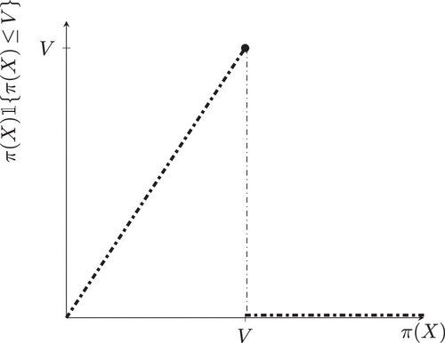
This is visualized in Figure 1. However, optimizing this function, which is nonconvex and discontinuous, is challenging (Mohri and Medina 2014, Huchette et al. 2020). Instead, we need to find a loss function that provides good prices when optimized using the samples we observe, Y and P, rather than valuations V.

1.3. Convex Relaxations and Impossibility Results

In particular, we aim to find loss functions that are convex, so they can be optimized efficiently yet still have provable guarantees on expected revenue relative to the optimal contextual pricing policy that has access to the valuation distribution, $p^{*}=\text{arg}\hspace{0.17em}{\text{max}}_{\pi }\mathcal{R}(\pi (X))$, where the dependence on X is henceforth omitted for notational clarity. We start by showing an impossibility result, which states that there is no loss function with access only to posted price data that is able to recover the optimal price for all valuation distributions. This proposition is a minor extension of theorem 2 of Mohri and Medina (2014), which proves that there is no convex surrogate for which the global minimum price is obtained in the case with access to valuation data. We denote a loss function using observational posted-price data as $L(\pi (X),Y,P):{\mathbb{R}}_{+}\times \{0,1\}\times {\mathbb{R}}_{+}\to \mathbb{R}$.

Proposition 1.

There is no nonconstant function ${\mathbb{E}}_{Y,P}[L(·,Y,P)|V=v]$, left continuous in v and with $L(·,Y,P)$ convex with respect to its first argument such that, for any distribution $(Y,P,V)\sim D$ on $\{0,1\}\times {\mathbb{R}}_{+}\times {\mathbb{R}}_{+}$ satisfying Equation (1), there exists a nonnegative optimal price $p^{*}\in \text{arg}\hspace{0.17em}{\text{max}}_p\mathcal{R}(p)$, satisfying ${\min }_p{\mathbb{E}}_{Y,P}[L(p,Y,P)]={\mathbb{E}}_{Y,P}[L(p^{*},Y,P)]$.

This is proved in Online Appendix A. The requirement of left continuity of the expected loss is a minor technical requirement that follows from a left-continuity assumption in Mohri and Medina (2014). Huchette et al. (2020) also show that optimizing the function ${\max }_{\theta }{\sum }_i〈\theta ,X_i〉\mathrm{𝟙}\{〈\theta ,X_i〉\le V_i\}$ is NP-hard in the setting in which valuation samples are available for the class of linear policies.

In general, it is difficult to further characterize the worst case expected revenue gap for an arbitrary convex loss function, and instead, we focus on analyzing the performance of specific convex loss functions inspired by pricing practice and the academic literature. However, for the case in which prices are restricted to a discrete price ladder (a common case studied in, e.g., Cohen et al. 2017) and under some additional minor technical assumptions, we can establish an upper bound on the worst case revenue ratio using MIP techniques.

1.4. An Upper Bound on Revenue for Discrete Pricing Using Mixed-Integer Programming

Suppose there are $p_1,p_2,\dots ,p_m$ fixed discrete prices with corresponding purchase probabilities ${\overline{F}}_1,{\overline{F}}_2,\dots ,{\overline{F}}_m$. Let $L_{i,j}^1$ and $L_{i,j}^0$ be the loss associated with prescribing a price $p_i$ to a customer who previously received price $p_j$ and purchased or did not purchase, respectively.³ In this discrete setting, we can formulate the problem of finding the worst case revenue ratio as

The objective in (3a) is to construct a loss function that maximizes the worst case ratio between the expected revenue of the prescribed price $p_s$ and that of the optimal price $p_{s^{*}}$. The prescribed price $p_s$ is selected as the one minimizing the expected loss as specified in Constraint (3b). The optimal price $p_{s^{*}}$, by contrast, is defined as the one maximizing expected revenue under the purchase probabilities $\overline{F}$ as shown in Constraint (3c).

We find the worst case across all log-concave distributions $\overline{F}$, which is encoded in Constraint (3e). Constraint (3f) also requires $\overline{F}$ to be a valid complementary CDF in that it is non-increasing and bounded between zero and one. Constraint (3d) enforces that L is strictly convex in the chosen price to rule out the degenerate solution in which L is constant and is, therefore, minimized by any price. We note that $ϵ$ can be made arbitrarily small. We also make the minor technical assumption that L is bounded (with the upper bound arbitrarily set to one) to permit a big-M reformulation of Constraint (3b).

This is a challenging bilevel nonconvex optimization problem. To find a tractable upper bound, instead of optimizing L over the worst case $\overline{F}$ from the set of all log-concave distributions, we can instead optimize over the worst case from a finite set of carefully chosen log-concave distributions, $\mathcal{F}≔{\overline{F}}^1,\dots ,{\overline{F}}^R$. This approach also has the advantage of making the problem linear (with integer variables) because L is the only remaining decision variable although additional auxiliary decision variables are introduced:

This is an epigraph reformulation. The binary variable $z_i^r$ is set to one if i is the price index that minimizes the expected loss function for distribution ${\overline{F}}^r$. This is enforced using the big-M technique in Constraint (4c), and this requires L to be bounded. The optimal revenue for each distribution, ${\mathcal{R}}^{*r}={\max }_{i\in [m]}{p}_i{\overline{F}}_i^r$, can be calculated off-line for each distribution and is, therefore, not a decision variable.

Proposition 2.

Let $Z^{UB}$ be the objective from optimizing Formulation (4) and $Z^{*}$ be the objective from optimizing (3). Then, $Z^{UB}\ge Z^{*}$.

This result follows immediately from optimizing over a subset of distributions in the inner minimization problem. The quality of this bound depends on how well the finite set, $\mathcal{F}$, represents the infinite set of all log-concave distributions.

To find a bound on the revenue ratio, we propose an iterative algorithm, formalized in Online Appendix A, involving (i) finding a loss function that performs well against the current set of distributions and (ii) finding distributions on which the incumbent loss will perform poorly to add to the set. To find these adversarial distributions, we present two approaches:

1. A search over beta distributions using sampling techniques.

2. A mixed-integer nonlinear programming (MINLP) approach to find worst case adversarial distributions.

The first approach has the advantage of being fast and useful early in the algorithm, but it loses effectiveness after many iterations as distributions against which the loss function performs poorly become harder to find. The MINLP approach is slow, but it is useful in later iterations.

1.5. A Lower Bound Using Mixed-Integer Nonlinear Programming

To find the worst case adversarial distribution for an incumbent loss function L, we can use MINLP. In particular, we fix $p_{s^{*}}$ as the revenue-maximizing price, $p_s$ as the minimizer of the expected loss function, and solve the following program:

We then repeat for all $m\times m$ combinations of possible optimal $p_{s^{*}}$ and prescribed prices $p_s$ to find the worst case distribution. This formulation has a nonlinear term $\log ({\overline{F}}_i)$ for each variable ${\overline{F}}_i$. This is modeled and solved using spatial branch and bound in Gurobi 11. Objective (5a) is a log-transform of the revenue ratio to avoid the additional nonlinearity because of the fractional term. Furthermore, the revenue ratio achieved for the worst case distribution for any fixed loss function is necessarily a lower bound on the worst case revenue bound as formalized in the following proposition.

Proposition 3.

Let $Z^{LB}$ be the objective from optimizing Formulation (5) and $Z^{*}$ be the objective from optimizing (3). Then, $e^{Z^{LB}}\le Z^{*}$.

By sequentially generating adversarial distributions from beta distributions and then solving Formulation (5), we can find an upper bound on the worst case revenue ratio of 0.8633 for a discrete pricing grid between $0 and $10 that increases in $1 increments. Additional implementation details can be found in Online Appendix A.2.

2. Pricing Hinge Loss Function

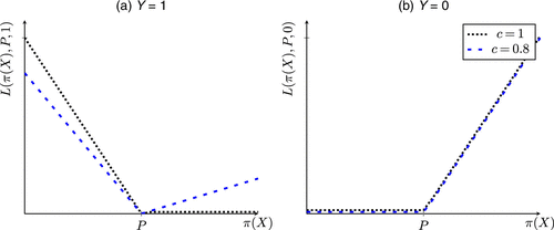
The loss functions computed in the previous section can be used when prices are discrete, whereas in this section, we propose a more intuitive loss inspired by pricing practice at Airbnb (Ye et al. 2018) that can be applied more generally to continuous settings. We first propose the hinge pricing loss function (see Figure 2), which has similarities to the hinge loss function used for classification tasks.

Definition 1.

The hinge pricing loss function is given by

$$L_c^h(\pi (X),Y,P)=\frac{1}{\varphi (P|X)}[cY{(P-\pi (X))}^{+}+(1-cY){(\pi (X)-P)}^{+}].$$

The parameter c is chosen by the seller as discussed later in this section. When $c=1$, $L_c^h$ penalizes prices that are below the listed price when the item was sold as well as prices that are above the listed price when the item wasn’t sold. Intuitively, if an item sold, the customer’s valuation is likely higher than the listed price, so pricing above the listed price is more attractive. Conversely, if an item did not sell, then the customer’s valuation is likely below the listed price, so pricing below this price should be encouraged. The parameter c controls how aggressive the pricing policy is. Having $c<1$ is important to achieve a reasonable pricing rule when the expected loss function is minimized (see Section 2.2).

Similar to inverse propensity scoring methods (Rosenbaum and Rubin 1983), each observation is scaled by a weight that is inversely proportional to the probability of receiving the price, $\varphi (P|X)$, to counteract the imbalance because of the historical pricing policy, allowing the analysis to proceed as if the historical pricing policy were uniform. In practice, a pricing policy from a sample can be found using empirical loss minimization as follows:

We also note that it is straightforward to extend to the case in which the historical pricing policy is a prior unknown but is estimated by using ${\widehat{\varphi }}_n(P_i|X_i)$ as a plug-in estimator for $\varphi (P_i|X_i)$. As long as the estimate ${\widehat{\varphi }}_n(P_i|X_i)$ is consistent and converges to $\varphi (P_i|X_i)$, the loss function is consistent and asymptotically converges to its expected value (Glynn and Quinn 2010). This justifies the use of plug-in estimates in large sample settings. However, as with other IPS methods, it can be biased in the finite sample setting (Dudík et al. 2014), but we show empirical evidence in Section 5 that the plug-in estimate performs well in practice.

2.1. Comparison with Ye et al. (2018)

The hinge pricing loss shares a similar motivation to the loss function from Ye et al. (2018), and in certain settings for extreme parameter choices, the loss functions are the same. Ye et al. (2018) propose a customized $ϵ$-insensitive loss used for contextual pricing at Airbnb:

This loss function is shown in Figure 3. Similar to the pricing hinge loss, this captures the intuition that, if the item sold, then the customer’s valuation is likely higher than the price the customer was offered, and the future price offered should be raised. However, the loss function from Ye et al. (2018) additionally introduces the idea that the price shouldn’t be raised too much because, eventually, the customer will not purchase if the price gets too high. This is reflected in the function in which there is no loss between P and $c_{1}P$, but an increasing loss is incurred above $c_{1}P$, where $c_1>1$. We note that, when $c<1$ for the hinge pricing loss, the penalty incurred when pricing above the sale price for items sold may have a similar effect. This gives the loss function a characteristic “U” shape (we highlight the similarity with $ϵ$-insensitive regression) compared with the hinge shape of the loss function we propose. Likewise, for the items that don’t sell, both loss functions incur a loss for pricing above the listed price at which no sale occurred, pressuring the price downward. However, the loss function from Ye et al. (2018) additionally incurs a loss for prices that are below $c_{2}P$, where $c_2<1$. The intuition is that, if the price is far below the customers’ valuation, there is potentially unrealized revenue. Another key distinction is that the loss from Ye et al. (2018) does not take into account the historical pricing policy, whereas the hinge loss divides by the propensity score $\varphi (P|X)$ to counteract the imbalance. As such, unless the historical pricing policy is uniformly distributed (such as would arise from a randomized trial), this is likely to affect the performance of this policy.

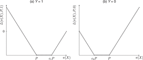
The approach from Ye et al. (2018) is intuitive and is shown to perform well in practice, but there are no guarantees on the expected revenue for the resulting policy, so it is unclear whether the additional arms that differentiate Ye et al. (2018) and the hinge loss are justified. However, because of the similarities between the two loss functions, we are able to provide revenue guarantees for the loss function from Ye et al. (2018) for a restricted class of settings. In particular, when the parameters in Ye et al. (2018) are set to $c_1=\infty$ and $c_2=-\infty$ and the historical pricing policy is uniform, then the loss proposed in Ye et al. (2018) is the same as the hinge pricing loss function for $c=1$.

2.2. Characterization of the Pricing Policy

We can characterize the behavior of the policy that results from using the hinge pricing loss function. When we minimize the conditional expectation of this loss function, we price at the conditional expected valuation for each customer, scaled by a parameter c, despite not observing the valuation data. This is proved in Lemma 1. As mentioned previously, the parameter c controls how aggressive the pricing policy is with $c<1$ resulting in prices less than the expected valuation and $c>1$ resulting in prices above the expected valuation. We focus on $c<1$ as this results in stronger revenue bounds. We provide guidance on how to choose c robustly following our analysis.

Lemma 1

(Hinge Pricing Loss Optimality Condition). Under Assumptions 1 and 2,

$$p_h=\text{arg}\hspace{0.17em}{\text{min}}_{\pi (X)}{\mathbb{E}}_{Y,P}\left[\frac{1}{\varphi (P|X)}\left(cY{(P-\pi (X))}^{+}+(1-cY){(\pi (X)-P)}^{+}\right)|X\right]=c\mathbb{E}[V|X].$$

This simple result is proved in Online Appendix B and is important because it provides clarity about the behavior of the pricing policy that results from minimizing the expected pricing hinge loss function and enables further analysis toward revenue bounds. This is not clear in previous loss functions used for pricing, such as Ye et al. (2018).

2.3. Expected Revenue Bounds

By maximizing the expected hinge pricing policy, we can find bounds on the optimal expected revenue relative to the best pricing policy that has access to the conditional valuation distribution and solves $p^{*}=\text{arg}\hspace{0.17em}{\text{max}}_p\mathcal{R}(p)$. Furthermore, these bounds are robust in the sense that this holds across all valuation distributions that satisfy the log-concave assumption, including an adversarially chosen distribution.

Theorem 1.

Let $p^{*}=\text{arg}\hspace{0.17em}{\text{max}}_p\mathcal{R}(p)$ and

$$p_h=\underset{\pi (X)}{\text{arg}\hspace{0.17em}\text{min}}{\mathbb{E}}_{Y,P}\left[\frac{1}{\varphi (P|X)}(cY{(P-\pi (X))}^{+}+(1-cY){(\pi (X)-P)}^{+})|X\right].$$

Under Assumptions 1–3, for $0<c\le 1$, the expected worst case revenue from pricing using the hinge loss function is bounded by

$$\frac{\mathcal{R}(p_h)}{\mathcal{R}(p^{*})}\ge \min \left\{\underset{z\le -2c}{\min }\frac{cz{e}^{-z(\frac{1}{c}-1)-1}}{z+c}, \underset{0<z<1}{\min }\frac{c(z-1)e^{c(z-1)}}{z\ln (z)}\right\}.$$

Furthermore, this bound is tight.

Sketch of the Proof

(Proven Formally in Online Appendix C). Consider two cases, corresponding to each term in the minimization: the case in which the prescribed price is below the optimal price for the adversarial distribution ($p_h<p^{*}$) and the case in which it is above ($p_h>p^{*}$). Which case is relevant depends on the chosen parameter of c. If a lower value of c is chosen (i.e., the price is much below the expected valuation), the adversary chooses a valuation distribution in which $p_h<p^{*}$, which is characterized by many high-valued customers that the lower price $p_h$ doesn’t fully exploit. This is shown in Figure 4, (a) and (b). For the special case in which $0\le c\le 0.5$, the adversarial distribution is simple and puts a point mass at $p^{*}$, so $\mathbb{E}[V|X]=p^{*}$, and the hinge price gets a fraction c of the revenue (see Online Appendix C.4). Conversely, if a higher value of c is chosen, the adversary chooses a distribution in which $p_h>p^{*}$, which is characterized by a sharp decline in selling probability above $p^{*}$, so the revenue at $p_h$ is lower. This is illustrated in Figure 4(c). A special case occurs when $c=1$, in which case the revenue bound is equal to $e^{-1}$ (see Online Appendix C, Corollary 6). This case is an application of lemma 5.4 in Lovász and Vempala (2007) and Grünbaum’s (1960) theorem.

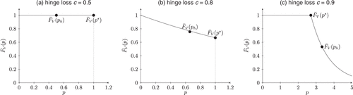
We note that Theorem 1 is tight, meaning that we can identify worst case distributions for all values of c that match the revenue bounds given in the theorem. These are given in Online Appendix D.

Although the bound from Theorem 1 is difficult to simplify analytically, numerical evaluation of the expressions in Theorem 1 leads to the following characterization of the worst case revenue:

Corollary 1.

${\max }_{0\le c\le 1}\frac{\mathcal{R}(p_h)}{\mathcal{R}(p^{*})}\ge 0.7715$, which occurs at $c^{*}=0.8234$.

These bounds can be compared with the bounds in Chen et al. (2023), who study a similar setting. In their single item setting, Chen et al. (2023) study pricing from transaction data with observations of the price of purchases. Under a slightly more general assumption of an increasing generalized failure rate but a more restrictive uniform historical pricing policy, they are able to show that their pricing policy achieves a 0.5 fraction of the optimal revenue. These bounds can also be compared with those in Chen et al. (2024), who study robust pricing when the mean of the valuation distribution is known but without the log-concavity assumption, and show that the revenue bound goes to zero for adversarial choice of the mean. The setting in which the mean is known is also studied in Elmachtoub et al. (2021), but under a different metric: the revenue ratio of the optimal single price relative to the optimal personalized pricing strategy.

This result provides the pricing practitioner with guidance on how to select c in a robust manner by balancing the risk that the valuation distribution is concentrated at high or low values. In particular, this suggests pricing at $c=0.8234$, which is the point at which the two bounds are equal and the adversary is ambivalent about choosing a distribution with an optimal price above or below $p_h$.

Furthermore, for many common valuation distributions, the relative revenue achieved is substantially greater than the worst case bound. In Proposition 4, proven in Online Appendix E, we show that, when customers have a uniform distribution of valuations between zero and an arbitrary maximum valuation, this pricing approach achieves 96.88% of the optimal revenue, using $c^{*}=0.8234$. This is equivalent to the canonical linear demand setting. When customer valuations follow an exponential distribution, equivalent to log-linear demand, this approach achieves 98.24% of the optimal revenue.

Proposition 4.

For the following customer valuation distributions, a tighter revenue ratio can be found when minimizing the expected hinge pricing loss function:

1. For $V\sim$ Uniform $(0,\overline{v})$, $\frac{\mathcal{R}(p_h)}{\mathcal{R}(p^{*})}=c(2-c)$. For $c^{*}=0.8234$, $\frac{\mathcal{R}(p_h)}{\mathcal{R}(p^{*})}=0.9688$.

2. For $V\sim$ Exponential $(\lambda )$, $\frac{\mathcal{R}(p_h)}{\mathcal{R}(p^{*})}=c{e}^{1-c}$. For $c^{*}=0.8234$, $\frac{\mathcal{R}(p_h)}{\mathcal{R}(p^{*})}=0.9824$.

3. Quantile Pricing Loss Function (No-Purchases Are Not Recorded)

We also propose an alternative loss function that is able to achieve similar, albeit slightly lower, worst case pricing but can be used in settings in which the no-purchase decision is not observed, and this is often the case with transaction data (e.g., Chen et al. 2023). The quantile loss is visualized in Figure 5.

Definition 2.

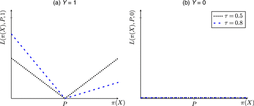
The quantile pricing loss function is given by

$$L_{\tau }^q(\pi (X),Y,P)=\frac{Y}{\varphi (P|X)}[(1-\tau ){(P-\pi (X))}^{+}+\tau {(\pi (X)-P)}^{+}].$$

This can be considered a weighted quantile loss function for price, using only data for which the product sold. As such, when this loss function is minimized, prices are prescribed at a given quantile of the historical prices of items that sold, depending on $\tau$. To the best of our knowledge, this loss function is not currently used in practice, but it does bear resemblance to some commonly used contextual pricing strategies, whereby the price is set to be close to similar products that have recently sold, in which “similar” here means at a given quantile of the price given. If the product doesn’t sell, there is no contribution to the loss.

3.1. Comparison with Chen et al. (2023)

The quantile loss has similarities to the loss function from Chen et al. (2023). Chen et al. (2023) study a similar problem of pricing from transaction data using observations of purchase prices, though their focus is on multi-product assortments rather than convexity or contextual information. In particular, for the single product setting, they propose maximizing the following function to obtain a pricing policy:⁴

This is visualized in Figure 6, (a) and (b). The rationale is that, if the customer purchased at a price P, the cutomer will purchase at any price below P, but Chen et al. (2023) take a conservative approach and assume there is no sale above P. They study a setting with transaction data in which only purchases are observed but not no-purchase outcomes. As such, they implicitly assume there is no contribution from the no-purchase decisions.

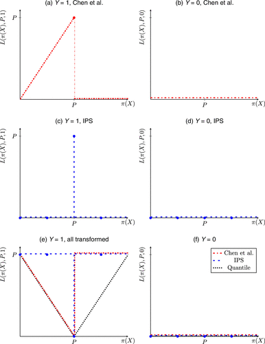
The loss function from Chen et al. (2023) can be transformed from a maximization to a minimization through multiplication by negative one and translate by a constant P to result in the loss function in Figure 6(e). Neither of these transformations affects the minimizer of the function. It is clear that this loss function is nonconvex and, therefore, potentially difficult to optimize in the contextual setting. The quantile pricing loss function can be thought of as a convex relaxation of this function in the sense that, rather than having a discontinuity at P, there is a linear penalty associated with increasing the price above this price as shown in Figure 6(e). This maintains the convexity of the loss function. This relaxation does not assume all revenue is lost above P, so it can be considered less conservative than Chen et al. (2023) although this also depends on the choice of $\tau$. In addition, the loss function in Chen et al. (2023) does not adjust for the historical pricing policy, and as such, revenue guarantees can be obtained only for the case of uniform pricing policies. However, it is possible that the model from Chen et al. (2023) could be extended to the more general historical pricing policies by using inverse propensity weighting because inverse propensity weighting allows the analysis to proceed as if the historical policy were uniform.

3.2. Comparison with Inverse Propensity Scoring

We also note the similarity between the quantile loss and an IPS approach (Rosenbaum and Rubin 1983, Beygelzimer and Langford 2009, Li et al. 2011). In a setting in which the price is discrete, the IPS estimator is

Here, there is a contribution to the reward proportional to $PY/\varphi \left(P\right|X)$ only if the proposed price $\pi (X)$ is equal to the price P that was given to the customer in the observed data. Thus, the reward obtained from a customer can be considered as a point mass at $\pi (X)=P$. This is shown in Figure 6, (c) and (d). Similarly, this can be transformed by multiplying by negative one and shifting by $PY/\varphi \left(P\right|X)$ as shown in Figure 6(e). We note that, rather than having a point mass, the quantile reward function has a linear penalty for prices above or below the point $\pi (X)=P$.

3.3. Characterization of the Pricing Policy

We can characterize the pricing policy that results from minimizing the expected conditional quantile pricing loss function in Lemma 2. This shows that, when this loss function is optimized, the price is set such that there is a fixed ratio between the total area under the valuation complementary CDF and the area below the complementary CDF and below the price. This is useful for proving revenue bounds because the total area under the complementary CDF is the maximum expected revenue achievable from a clairvoyant seller who uses first degree price discrimination.

Lemma 2

(Quantile Optimality Condition). Under Assumptions 1 and 2, when only purchases are observed,

$$\frac{{\int }_0^{p_q}{\overline{F}}_V(p)dp}{{\int }_0^{\infty }{\overline{F}}_V(p)dp}=1-\tau ,$$

where $p_q=\text{arg}\hspace{0.17em}{\text{min}}_{\pi (X)}{\mathbb{E}}_{Y,P}[\frac{Y}{\varphi (P|X)}((1-\tau ){(P-\pi (X))}^{+}+\tau {(\pi (X)-P)}^{+})|X]$.

This is proved in Online Appendix F. It is also important to differentiate $L_{\tau }^q$ from the standard quantile loss function applied to the (unobserved) valuation data, which is similar to the approach taken by Allouah et al. (2021). If we applied quantile regression here, we would get an estimator of the fraction of the area under the valuation PDF, ${\int }_0^{p_q}{f}_V\left(p\right)dp/{\int }_0^{\infty }{f}_V\left(p\right)dp=\tau$, resulting in a different policy where ${\overline{F}}_V(p_q)=1-\tau$.

3.4. Expected Revenue Bounds

When we optimize the quantile pricing loss function, we can find bounds on the optimal revenue relative to the best contextual pricing policy that has access to the valuation distribution.

Theorem 2.

Let $p^{*}=\text{arg}\hspace{0.17em}{\text{max}}_p\mathcal{R}(p)$ and

$$p_q=\underset{\pi (X)}{\text{arg}\hspace{0.17em}\text{min}}{\mathbb{E}}_{Y,P}\left[\frac{Y}{\varphi (P|X)}((1-\tau ){(P-\pi (X))}^{+}+\tau {(\pi (X)-P)}^{+})|X\right].$$

Under Assumptions 1–3, for $0<\tau \le 1$, the expected worst case revenue from pricing using the quantile loss function can be bounded:

$$\frac{\mathcal{R}(p_q)}{\mathcal{R}(p^{*})}\ge \min \left\{\underset{\tau \le z\le 1}{\min }\frac{z\tau (\ln (z)+1)-z^2}{\tau -z},\underset{0<z<1}{\min }\frac{(1-\tau )(z-1)e^{(1-\tau )(z-1)}}{z\ln (z)}\right\}.$$

Similar to the hinge pricing loss function, the proof for Theorem 2 requires exploring two cases: one in which the price chosen by minimizing the quantile pricing loss is above the optimal price and one in which it is below. If $0.5\le \tau <1$, then the revenue bound simplifies to $\mathcal{R}\left(p_q\right)/\mathcal{R}\left(p^{*}\right)\ge 1-\tau$. Theorem 2 is formally proved in Online Appendix G.

Corollary 2.

${\max }_{0\le \tau \le 1}\frac{\mathcal{R}(p_q)}{\mathcal{R}(p^{*})}\ge 0.749$, which occurs at ${\tau }^{*}=0.209$.

Thus, the best worst case guarantee corresponds to setting the price to approximately the ${79}^{th}$ percentile of the items that sold. The complete relationship between the revenue bounds and $\tau$ is shown in Figure 7, which gives practitioners an idea of the worst case revenue for different choices of $\tau$. This bound is marginally weaker than the bound for the hinge pricing loss function, but it is applicable in the setting in which only sale outcomes are observed. In this respect, a fairer comparison would be with the 0.5 bound from Chen et al. (2023).

Corollary 3.

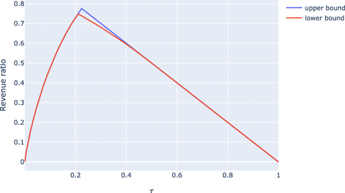
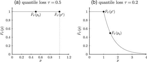
Theorem 2 is tight for $\tau \in (0,0.209)\cup (0.5,1]$.

For the quantile pricing loss function, we have identified the distributions that match the lower bound given in Theorem 2 for $0<\tau \le 0.209$ and $0.5\le \tau \le 1$ and show them in Figure 8. We formally describe them in Online Appendix D. It is unclear whether there exists an alternative valuation distribution that meets the lower bound for the range $0.209<\tau \le 0.5$ or whether it is possible to improve the bound for this range, but we can obtain a simple upper bound for this range using the point-mass distribution in Figure 8(a). The difference between the upper bound and the lower bound from Theorem 2 is shown in Figure 7. We note that the difference is at most 0.027, so the bound is very close to being tight. More practically, there is minimal effect on the optimal choice for a robust $\tau$.

As with the pricing hinge loss function, we can show that, for common valuation distributions, the revenue achieved is substantially greater than against the worst case distribution. This is shown in Proposition 5 and proved in Online Appendix H.

Proposition 5.

For the following customer valuation distributions, a tighter revenue ratio can be found when minimizing the expected quantile loss function:

1. For $V\sim$ Uniform $(0,\overline{v})$, $\frac{\mathcal{R}(p_h)}{\mathcal{R}(p^{*})}=4(\sqrt{\tau }-\tau )$. For ${\tau }^{*}=0.209$, $\frac{\mathcal{R}(p_h)}{\mathcal{R}(p^{*})}=0.9927$.

2. For $V\sim$ Exponential $(\lambda )$, $\frac{\mathcal{R}(p_h)}{\mathcal{R}(p^{*})}=-e^1\tau \ln (\tau )$. For ${\tau }^{*}=0.209$, $\frac{\mathcal{R}(p_h)}{\mathcal{R}(p^{*})}=0.8893$.

4. Cross-Validation for Parameter Selection

The parameters c and $\tau$ can be chosen to robustly maximize revenue across all valuation distributions as per Corollary 1 or 2. However, this is often too conservative in practice. We present a simple heuristic for choosing c and $\tau$ for the specific data set encountered based on ideas from cross-validation. To evaluate the effectiveness of the model parameters, we propose using a demand model estimated from the available data. Specifically, for each parameter value ${\tau }_k$ in a discretized set of size K, we find an optimal policy ${\widehat{\pi }}_{{\tau }_k}$ by optimizing the corresponding hinge or quantile loss function. We then estimate the revenue obtained from this pricing policy using the estimated demand model and pick the parameter that corresponds to the highest estimated revenue. This approach allows us to utilize an accurate nonparametric demand model (such as a tree ensemble or neural network) without being concerned about the difficulty of optimizing such a nonconvex model. There are many choices for how to estimate the nonparametric demand model, but for the numeric experiments in Section 5, we use gradient-boosted trees, which are known to have state-of-the-art accuracy on tabular data (Shwartz-Ziv and Armon 2022). We minimize the binary cross-entropy loss,

with appropriate regularization of the boosted tree as discussed in Ke et al. (2017). Here, $\widehat{f}(X,P)\approx P(Y=1|P,X)$ is the conditional estimate for the probability of purchase given the price and features, whereas $\mathcal{T}$ is the class of gradient-boosted trees.

Algorithm 1

(Cross-Validation for Contextual Pricing)

Estimate demand model $\widehat{f}(X,P)$ from data, for example, using gradient boosted trees estimated via Equation (7);

for $k\in \{1,\dots ,K\}$ do

  Find the optimal policy using parameter ${\tau }_k$, ${\widehat{\pi }}_k=\text{arg}\hspace{0.17em}{\text{min}}_{\pi \in \mathrm{\Pi }}\frac{1}{n}{\sum }_{i=1}^n{L}_{{\tau }_k}(\pi (X_i),Y_i,P_i)$;

  Evaluate estimated reward $\widehat{{\mathcal{R}}_k}=\frac{1}{n}{\sum }_{i=1}^n{\widehat{\pi }}_k(X_i)\widehat{f}(X_i,{\widehat{\pi }}_k(X_i))$;

end

Find maximum reward $k^{*}=\text{arg}\hspace{0.17em}{\text{max}}_k\widehat{{\mathcal{R}}_k}$, choose ${\pi }_{k^{*}}$ as policy.

5. Numerical Experiments

We test the proposed loss functions using synthetic and real-world data sets. We benchmark against commonly used direct method approaches that first estimate demand using logistic regression (dm_log, e.g., Chen et al. 2021) and a tree ensemble model (dm_lgbm, e.g., Mišić 2020), then optimize estimated revenue to find a pricing policy. In particular, we adopt the logistic regression model implemented in sci-kit learn (Pedregosa et al. 2011) and the lightgbm gradient boosted tree package (Ke et al. 2017) with default parameters in each case. We also benchmark against an inverse propensity weighting approach (kern_ipw) adapted to the continuous action setting (Kallus and Zhou 2018) whereby revenue is estimated using a weighted average according to how far the historical price is from the proposed policy as evaluated by a Gaussian kernel. We benchmark against the model-free assortment approach from Section 3.1 (Chen et al. 2023, chen) and the approach from Section 2.1 (Ye et al. 2018, airbnb) used at Airbnb. We also benchmark against an inverse propensity score weighted version of this loss, airbnb_ipw, when the historical price is feature dependent. The hinge and quantile pricing loss functions (denoted hinge and quant, respectively) are optimized using the cross-validation technique from Section 4 to find the parameters ($\tau$ and c) from 10 evenly spaced candidate values between zero and one. We use the lightgbm model to evaluate the reward in this procedure. To find the bandwidth parameter for kern_ipw, we use the same cross-validation procedure over the same range. Likewise, to find the parameters $c_1$ and $c_2$ for airbnb and airbnb_ipw, we use the same cross-validation procedure with nine values for a comparable computational burden. This results in three equally spaced values between one and two for $c_1$ and three equally spaced values between zero and one for $c_2$ with all combinations taken. In all algorithms, the optimal policy is found using the popular Broyden–Fletcher–Goldfarb–Shanno (BFGS) nonlinear optimization algorithm (Nocedal and Wright 2006), implemented in scipy. This can handle nondifferentiable demand functions, such as tree-based ensemble methods.

5.1. Synthetic Data

Synthetic experiments are important in this setting because of the lack of publicly available pricing data with counterfactual outcomes on whether a customer would have purchased if a different price had been offered. As a result, estimating the revenue of different pricing policies from historical data is challenging. However, with synthetic data, the underlying probability distributions that govern customer behavior are known, so pricing policies can be evaluated.

In our synthetic experiments, we propose a number of different data-generating scenarios to test the algorithms under varied demand settings. We study two specifications for the valuation distribution: a linear model, $V_i=X_i+1+{ϵ}_i$, and a nonlinear step function, $V_i=3·1\{X_i\ge 1.75\}+1+{ϵ}_i$. In both settings, $X_i\sim \text{Uniform}(1,2)$ and ${ϵ}_i\sim \text{Uniform}(-1,1)$. The step function models a situation in which there is a threshold that represents a significant change in consumer behavior (e.g., willingness to pay may change significantly once retirement age is reached), whereas the linear case represents a proportional change (e.g., income and willingness to pay). We study a setting with and without (observed) price confounding. In the case with confounding, the historical pricing policy has a step function dependence on $X_i$, in which one group is given mainly high prices, whereas another group is given mainly low prices, via the following conditional density function:

In this setting, we also study the effectiveness of using a plug-in estimator of $\varphi (P_i|X_i)$. To estimate the conditional price density, we use Bayes theorem, $\widehat{\varphi }\left(P_i\right|X_i)=\widehat{f}(P_i,X_i)/\widehat{f}(X_i)$, where $\widehat{f}(P_i,X_i)$ and $\widehat{f}(X_i)$ are the joint and marginal distributions, respectively. To estimate each, we use kernel density estimation with an Epanechnikov kernel and fivefold cross-validation. We also study when the historical price is uniform $\varphi (p|X_i)=0.2,$ for $0\le p\le 5$, to imitate the setting of pricing following a period of price experimentation.

To ensure that the price optimization problem is convex, we study a class of linear pricing policies $\pi (X_i)={\theta }_0+{\theta }_1{X}_i$. This results in some model misspecification in the setting with nonlinear valuations. We compare the pricing policies generated to the optimal linear policy in each scenario, found by solving ${\pi }^{*}=\text{arg}\hspace{0.17em}{\text{max}}_{\pi \in \mathrm{\Pi }}\frac{1}{n}{\sum }_{i=1}^n\pi (X_i)\mathrm{𝟙}\{\pi (X_i)\le V_i\}$ directly, where $\mathrm{\Pi }$ is the class of linear functions.⁵ We report the average regret for the proposed pricing policy as the difference in revenue, $\frac{1}{n}{\sum }_{i=1}^n({\pi }^{*}(X_i)\mathrm{𝟙}\{{\pi }^{*}(X_i)\le V_i\}-\widehat{\pi }(X_i)\mathrm{𝟙}\{\widehat{\pi }(X_i)\le V_i\})$. We vary the data set size according to $n\in \{30,300,\mathrm{3,000},\mathrm{30,000}\}$. To initialize the BFGS optimizer, we use an initial solution ${\theta }_0,{\theta }_1=\frac{1}{2}$. We repeat each simulation 10 times and report the average with plus/minus one standard error.

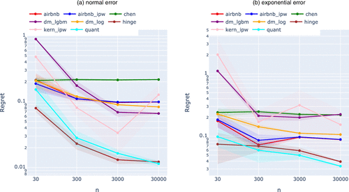
To show robustness to the error distribution, we repeat the simulations for the setting with the step function dependence of $V_i$ on $X_i$ and no confounding but with ${ϵ}_i\sim \text{Normal}(0,0.5)$ and ${ϵ}_i\sim \text{Exponential}(2)$.

5.1.1. Discussion.

In Figure 9, we observe the results in which the propensity scores are known, whereas Figure 10 shows the results for the setting with confounding and estimated propensity scores. In all cases, we observe that the hinge and quantile pricing loss functions are competitive with and, in some cases, outperform state-of-the-art benchmarks.

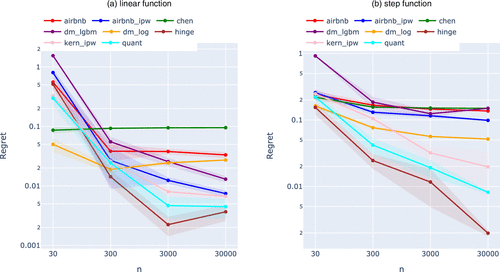
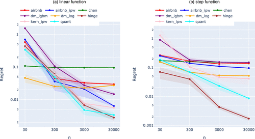
When the valuation data are linear, for small data sets with $n=30$ and $n=300$, the logistic regression direct method performs relatively well. This is potentially because of the low model complexity of logistic regression and only minor model misspecification (the logistic function cannot exactly model the uniform complementary CDF). For small data sets, the gradient-boosted tree and kernel approaches are highly nonlinear and do not converge to a high-quality solution. We note that none of the approaches we benchmark against except airbnb and airbnb_ipw results in a convex policy optimization problem, so it is possible that any approach could get stuck at a local minimum, an issue that the hinge and quantile pricing loss functions do not have.

However, for larger data sets with $n=3,000$ and $n=3,00,000$, we observe that the other methods improve, whereas the logistic regression does not. For larger data sets, gradient-boosted trees and kernel approaches can accurately learn the demand function, whereas the logistic regression retains a small bias. Furthermore, gradient-boosted trees and kernels generally become smoother and easier to optimize with more data.

When the valuation data has a step function in X, the logistic regression’s bias is greater, and it performs worse for all data sets. We observe that the quantile and hinge pricing models perform particularly well in this nonlinear setting. We also observe similar trends with and without price confounding, suggesting that the inverse propensity scores can be estimated sufficiently well for this example. We also do not observe substantial differences with different error distributions in Figure 11, indicating a robustness to distribution.

We also observe that the hinge and quantile pricing models tend to choose better policies than the boosted tree model itself. This is likely because optimizing the boosted tree is very challenging because of nonconvexity, whereas for each parameter instance in the cross-validation, the hinge and quantile regressions are convex. Furthermore, we emphasize that the hinge and quantile pricing loss algorithms have guarantees on expected revenue, whereas the algorithms we benchmark against do not.

In Online Appendix I, we study the case in which the overlap assumption is violated but use the strategy from Sachdeva et al. (2020) to restrict prescribing prices for which there is no overlap. We show that, when the optimal price still has coverage, the results are similar to the other experiments.

5.2. Semisynthetic Case Study: Personalized Prices for Groceries

We also evaluate the proposed contextual pricing approaches based on a data set of purchases of grocery products. There is significant recent interest in personalized pricing for grocery stores with Senators Elizabeth Warren and Bob Casey recently writing a letter to the chairman and CEO of Kroger Company to clarify the company’s use of electronic shelving labels and artificial intelligence in pricing products.⁶ The data we have tracks individual customers and whether they purchased strawberries from a chain of grocery stores at the posted price. In addition, demographic data are collected on the individual customers based on enrollment in a loyalty program, specifically, income, age, gender, marital status, home ownership, size of household, and whether the customer has children. These data were collected by the analytics firm Dunnhumby, and we use the cleaned and processed version of the data from Amram et al. (2022), who provide a detailed description of the data. The data size is 97,295 rows, corresponding to unique customer trips to the supermarket, with $3.49\%$ of trips resulting in a sale of strawberries. Once the features described above have been one-hot encoded, it results in a data set with dimension $m=34$.

Using this data, Amram et al. (2022) and Biggs et al. (2021b) investigate the potential of offering personalized prices to customers based on specific features to maximize revenue, employing interpretable tree-based models. However, because of the possibility of unobserved confounding—because the data lacks information on competitor pricing—we focus on comparing the relative performance of different methodologies rather than attempting to precisely estimate the potential revenue gains from personalized pricing. The empirical gains from personalized pricing have already been explored in detail by Dubé and Misra (2023) using data from a randomized control trial.

To evaluate the relative performance, we employ a semisynthetic approach so that the exact relationship between the variables is known. The variables X and P are as given in the data, but new sales observations Y are generated, according to a conditional outcome distribution of Y given X and P estimated using a gradient-boosted tree model trained on a held-out data set. We refer to this data set as the evaluation data set, whereas the remainder of the data, with size n, is used to train the pricing policies and is referred to as the prescription data set. Finally, the revenue from the policies is evaluated based on the revenue according to the known conditional outcome distribution. The historical pricing policy is not known but is estimated from the data using a log-normal distribution. This pricing policy has no dependence on customer features X because the grocery is not currently using personalized pricing.

In Figure 12, we show the revenue of different policies. We repeat the experiment 10 times for each randomly sampled prescription data set of size $n=2,000,5,000,10,000,20,000$. We restrict all pricing policies to be in the range of observed prices [0, 5].

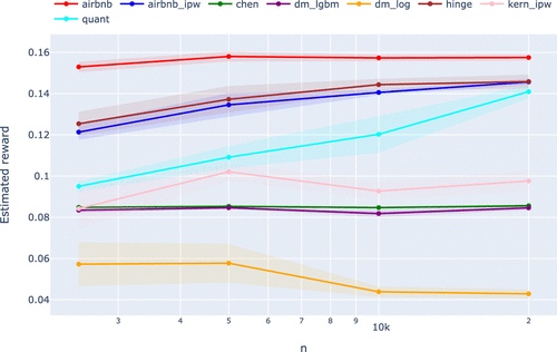
We observe that the convex pricing loss functions perform better than the other benchmarks on this data set. In particular, airbnb pricing loss function performs the best across all data set sizes with the airbnb_ipw, hinge, and quantile pricing loss functions improving to comparable performance for larger data sets. This suggests that there are practical advantages to the loss function from Ye et al. (2018) and that further understanding the theoretical revenue guarantees for this function class is a worthwhile avenue for future work.

6. Extensions

We provide several extensions to the model that incorporate a range of potential scenarios a pricing practitioner might encounter:

1. Learning from adaptive historical pricing policies: Another setting of practical interest is one in which the historical pricing algorithm learns from previously observed pricing trajectories for different projects, so the historical pricing policy is not constant in time. The methodology extends naturally from existing results, but there are many practical challenges in estimating the historical pricing policy, discussed in detail in Online Appendix J.

2. No observed low prices: In the case in which low prices are not covered by the historical policy (i.e., the range of prices given by the historical policy is bounded away from zero), a shift involving the lower bound on price needs to be made to the policy to achieve the same pricing rule.

Corollary 4.

Suppose $\varphi (p|X)>0$ only for $p\in [\underset{¯}{p},\overline{p}]$, and $\underset{¯}{p}\le \underset{¯}{v}\le \overline{v}\le \overline{p}$. Let $p_h=\text{arg}\hspace{0.17em}{\text{min}}_p\mathbb{E}[L_c^h(p,Y,P)|X]$. Define a shifted pricing policy as $p_h^{\prime }=p_h-\underset{¯}{p}(1-c)$. Then, $p_h^{\prime }=c\mathbb{E}[V|X]$.

This is proved in Online Appendix K but follows from a similar proof to Lemma 1. For the pricing quantile loss function, we provide a minor adjustment to the loss function in Online Appendix K and show that this achieves the same pricing rule.

• iii. Multiple products: We can extend the pricing hinge loss function to a scenario with multiple products and performance guarantees, which is explored in Online Appendix I. In particular, we use the assortment pricing setup from Chen et al. (2023), in which each customer buys the product with the highest utility from a fixed set of S products offered. Under an assumption that the product with the highest average valuation also has the highest potential revenue (satisfied, for example, if there is a hierarchy of stochastic dominance among product valuations), we can derive a lower bound on the revenue ratio relative to the optimal strategy.

• iv. Finite-sample bounds: The bounds introduced in Theorems 1 and 2 apply when optimizing the expected loss function. In practice, it is of interest to study how different the loss of the finite sample solution is. In Online Appendix M, we present finite sample bounds for linear policy classes before extending to kernel-based policies that can capture a more general nonlinear policy class.

7. Conclusions and Future Work

We propose methods to address the problem of contextual pricing using observational posted-price data rather than the well-studied setting in which willingness to pay (valuation) data are available. We focus on pricing algorithms that can achieve bounds on expected revenue and can also be computed tractably. In particular, we propose two loss functions, the quantile and hinge pricing loss functions, which are convex and can be easily optimized. We also show how to choose the relevant parameters to optimize bounds on expected revenue according to an adversarially chosen valuation distribution and how to heuristically choose parameter values when the seller has access to an estimated demand model that is accurate but challenging to optimize, such as a neural network or tree ensemble. Numerically, we show that the proposed loss functions are competitive against commonly used contextual pricing approaches, which are known to work well in practice but do not have theoretical expected revenue bounds and may be unpredictable because of nonconvexity. Going forward, it would be valuable to (i) derive revenue guarantees that hold in finite-sample regimes and (ii) examine how inaccuracies in estimating historical price likelihoods affect revenue bounds.

References

- (2023) Pricing for heterogeneous products: Analytics for ticket reselling. Manufacturing Service Oper. Management 25(2):409–426.Link, Google Scholar
- (2021) Revenue maximization from finite samples. Proc. 22nd ACM Conf. Econom. Comput. (ACM, New York), 51.Google Scholar
- (2023) Optimal pricing with a single point. Management Sci. 69(10):5866–5882.Link, Google Scholar
- (2014) Repeated contextual auctions with strategic buyers. Adv. Neural Inform. Processing Systems, vol. 27 (Curran Associates Inc., Red Hook, NY).Google Scholar
- (2022) Optimal policy trees. Machine Learn. 111(7):2741–2768.Crossref, Google Scholar
- (2015) Moving towards best practice when using inverse probability of treatment weighting (IPTW) using the propensity score to estimate causal treatment effects in observational studies. Statist. Medicine 34(28):3661–3679.Crossref, Google Scholar
- (2013) Optimal and efficient parametric auctions. Proc. 24th Annual ACM-SIAM Sympos. Discrete Algorithms (SIAM, Philadelphia), 596–604.Google Scholar
- (2020) Detecting customer trends for optimal promotion targeting. Manufacturing Service Oper. Management 25(2):448–467.Link, Google Scholar
- (2018) Are two (samples) really better than one? Proc. 2018 ACM Conf. Econom. Comput. (ACM, New York), 175–175.Google Scholar
- (2005) Log-concave probability and its applications. Econom. Theory 26(2):445–469.Crossref, Google Scholar
- (2020) Confidence intervals for data-driven inventory policies with demand censoring. Oper. Res. 68(2):309–326.Abstract, Google Scholar
- (2006) Convexity, classification, and risk bounds. J. Amer. Statist. Assoc. 101(473):138–156.Crossref, Google Scholar
- (2011) Robust monopoly pricing. J. Econom. Theory 146(6):2527–2543.Crossref, Google Scholar
- (2020) From predictive to prescriptive analytics. Management Sci. 66(3):1025–1044.Link, Google Scholar
- (2009) The offset tree for learning with partial labels. Proc. 15th ACM SIGKDD Internat. Conf. Knowledge Discovery Data Mining (ACM, New York), 129–138.Google Scholar
- (2021) Improved revenue bounds for posted-price and second-price mechanisms. Oper. Res. 69(6):1805–1822.Link, Google Scholar
- (2021a) Loss functions for discrete contextual pricing with observational data. Preprint, submitted November 18, https://arxiv.org/abs/2111.09933.Google Scholar
- (2021b) Model distillation for revenue optimization: Interpretable personalized pricing. Internat. Conf. Machine Learn. (PMLR, New York), 946–956.Google Scholar
- (2022) Offline pricing and demand learning with censored data. Management Sci. 69(2):885–903.Google Scholar
- (2021) Assortment optimization under the decision forest model. Preprint, submitted March 26, https://doi.org/10.2139/ssrn.3812654.Google Scholar
- (2022) Distribution-free pricing. Manufacturing Service Oper. Management 24(4):1939–1958.Link, Google Scholar
- (2024) Screening with limited information: A dual perspective. Oper. Res. 72(4):1487–1504.Link, Google Scholar
- (2023) Model-free assortment pricing with transaction data. Management Sci. 69(10):5830–5847.Link, Google Scholar
- (2021) A statistical learning approach to personalization in revenue management. Management Sci. 68(3):1923–1937. Link, Google Scholar
- (2020) Feature-based dynamic pricing. Management Sci. 66(11):4921–4943.Link, Google Scholar
- (2015) Pricing with limited knowledge of demand. Technical report, National Bureau of Economic Research, Cambridge, MA.Google Scholar
- (2017) The impact of linear optimization on promotion planning. Oper. Res. 65(2):446–468.Link, Google Scholar
- (2014) The sample complexity of revenue maximization. Proc. 46th Annual ACM Sympos. Theory Comput. (ACM, New York), 243–252.Google Scholar
- (2020) More revenue from two samples via factor revealing SDPs. Proc. 21st ACM Conf. Econom. Comput. (ACM, New York), 257–272.Google Scholar
- (2015) Dynamic pricing and learning: Historical origins, current research, and new directions. Surveys Oper. Res. Management Sci. 20(1):1–18.Crossref, Google Scholar
- (2016) The sample complexity of auctions with side information. Proc. 48th Annual ACM Sympos. Theory Comput. (ACM, New York), 426–439.Google Scholar
- (2015) Revenue maximization with a single sample. Games Econom. Behav. 91:318–333.Crossref, Google Scholar
- (2017) Scalable price targeting. Technical report, National Bureau of Economic Research, Cambridge, MA.Google Scholar
- (2023) Personalized pricing and consumer welfare. J. Political Econom. 131(1):131–189.Crossref, Google Scholar
- (2014) Doubly robust policy evaluation and optimization. Statist. Sci. 29(4):485–511.Crossref, Google Scholar
- (2021) The value of personalized pricing. Management Sci. 67(10):6055–6070.Link, Google Scholar
- (2021) Customer choice models vs. machine learning: Finding optimal product displays on Alibaba. Oper. Res. 70(1):309–328.Link, Google Scholar
- (2016) Analytics for an online retailer: Demand forecasting and price optimization. Manufacturing Service Oper. Management 18(1):69–88.Link, Google Scholar
- (2010) An introduction to the augmented inverse propensity weighted estimator. Political Anal. 18(1):36–56.Crossref, Google Scholar
- (1960) Partitions of mass-distributions and of convex bodies by hyperplanes. Pacific J. Math. 10(4):1257–1261.Crossref, Google Scholar
- (1986) Statistics and causal inference. J. Amer. Statist. Assoc. 81(396):945–960.Crossref, Google Scholar
- (2018) Making the most of your samples. SIAM J. Comput. 47(3):651–674.Crossref, Google Scholar
- (2020) Contextual reserve price optimization in auctions via mixed integer programming. Larochelle H, Ranzato M, Hadsell R, Balcan MF, Lin H, eds. Adv. Neural Inform. Processing Systems, vol. 33 (Curran Associates, Inc., Red Hook, NY), 1287–1297.Google Scholar
- (2018) Policy evaluation and optimization with continuous treatments. Internat. Conf. Artificial Intelligence Statist. (PMLR, New York), 1243–1251.Google Scholar
- (2017) LightGBM: A highly efficient gradient boosting decision tree. Adv. Neural Inform. Processing Systems (Curran Associates Inc., Red Hook, NY), 3146–3154.Google Scholar
- (2008) Exploration scavenging. Proc. 25th Internat. Conf. Machine Learn. (ACM, New York), 528–535.Google Scholar
- (2011) Unbiased offline evaluation of contextual-bandit-based news article recommendation algorithms. Proc. Fourth ACM Internat. Conf. Web Search Data Mining (ACM, New York), 297–306.Google Scholar
- (2007) The geometry of logconcave functions and sampling algorithms. Random Structures Algorithms 30(3):307–358.Crossref, Google Scholar
- (2023) Personalized pricing with invalid instrumental variables: Identification, estimation, and policy learning. Preprint, submitted February 24, https://arxiv.org/abs/2302.12670.Google Scholar
- (2020) Optimization of tree ensembles. Oper. Res. 68(5):1605–1624.Link, Google Scholar
- (2014) Learning theory and algorithms for revenue optimization in second price auctions with reserve. Internat. Conf. Machine Learn. (PMLR, New York), 262–270.Google Scholar
- (2017) Revenue optimization with approximate bid predictions. Adv. Neural Inform. Processing Systems, vol. 30 (Curran Associates Inc., Red Hook, NY).Google Scholar
- (2006) Numerical Optimization (Springer Science & Business Media, New York).Google Scholar
- (2011) Scikit-learn: Machine learning in Python. J. Machine Learn. Res. 12(85):2825–2830.Google Scholar
- (1983) The central role of the propensity score in observational studies for causal effects. Biometrika 70(1):41–55.Crossref, Google Scholar
- (2020) Off-policy bandits with deficient support. Proc. 26th ACM SIGKDD Internat. Conf. Knowledge Discovery Data Mining (ACM, New York), 965–975.Google Scholar
- (2022) Tabular data: Deep learning is not all you need. Inform. Fusion 81:84–90.Crossref, Google Scholar
- (2023) Context-based pricing for revenue optimization with applications to the airline industry. Annual Hawaii Internat. Conf. System Sci.Google Scholar
- (2015) Counterfactual risk minimization: Learning from logged bandit feedback. Internat. Conf. Machine Learn. (PMLR, New York), 814–823.Google Scholar
- (2025) Offline feature-based pricing under censored demand: A causal inference approach. Manufacturing Service Oper. Management 27(2):535–553.Google Scholar
- (2018) Customized regression model for Airbnb dynamic pricing. Proc. 24th ACM SIGKDD Internat. Conf. Knowledge Discovery Data Mining (ACM, New York), 932–940.Google Scholar