Gradient Descent for Unbounded Convex Functions on Hadamard Manifolds and Its Applications to Scaling Problems

1. Introduction

In convex optimization, it is typically assumed that the objective function f is bounded below. The performance of a minimization algorithm is evaluated by its convergence behavior to the minimum of f. This paper addresses the convergence behavior of minimization algorithms for a “lower-unbounded” convex function f, that is, $\inf \hspace{0.17em}f(x)=-\infty$. This may look meaningless, because the trajectory $x_i$ of an algorithm diverges to infinity, and $f(x_i)$ goes to $-\infty$. The meta question of the paper is the following:

What can we gain from such a divergent sequence?

Let us formalize our setting and mention its background. Let M be a Hadamard manifold—a simply connected complete Riemannian manifold with nonpositive sectional curvature. Let $f:M\to \mathbb{R}$ be a (twice differentiable) geodesically convex function, that is, f is convex along any geodesic. We consider the following unconstrained convex optimization problem on M:

Such a problem setting is significant in the recent progress on operator scaling (Gurvits [27]) and generalizations (see Allen-Zhu et al. [1], Bürgisser et al. [12], Bürgisser et al. [13], Garg and Oliveira [21], Garg et al. [22, 23], and Hirai et al. [34]). In the classical matrix scaling (Sinkhorn [58]), the scalability is equivalent to the boundedness of (1.1) for some convex function f in ${\mathbb{R}}^n$. Further, it is also equivalent to the perfect-matching condition of the associated bipartite graph. Hayashi et al. [29] studied asymptotic behavior of the Sinkhorn algorithm for the unscalable (unbounded) case, and revealed that a combinatorial certificate (Hall blocker) of unscalability can be identified from divergent behavior of the Sinkhorn algorithm. Although a Hall blocker is easily obtained by network-flow algorithms, finding the corresponding certificate (shrunk subspace) for the operator scaling setting is possible but quite difficult (see Hamada and Hirai [28], Ivanyos et al. [37, 38]). Just recently, Franks et al. [19] modified the operator Sinkhorn algorithm—an alternating minimization algorithm for some convex function on the Hadamard manifold of positive definite matrices—to obtain a shrunk subspace in polynomial time, although it is still rather complicated. The matrix and operator scaling problems are generalized to a class of convex optimization involving reductive group actions, called noncommutative optimization (Bürgisser et al. [13]), which asks to minimize the Kempf-Ness function associated with an orbit of the action. This is formulated as a convex optimization problem on a representative class of Hadamard manifolds—symmetric spaces of nonpositive curvature. It is lower-unbounded if and only if the orbit is unstable, where a 1-parameter subgroup (destabilizing 1-PSG) in the Hilbert-Mumford criterion is the unboundedness certificate that generalizes a Hall blocker and a shrunk subspace. As mentioned in Bürgisser et al. [13], it is a great challenge to design polynomial-time algorithms for several noncommutative optimization problems, such as (un)stability determination, moment polytope membership, and orbit-closure intersection, which will bring fruitful applications to broader areas of mathematical sciences. Many of them involve (un)bounded determination of Kempf-Ness functions, though our current knowledge on such problems is limited.

Motivated by these considerations, we study minimization of lower-unbounded convex functions on Hadamard manifolds. Even in the Euclidean setting $M={\mathbb{R}}^n$, there are few works (see, e.g., Auslender [4] and Obuchowska [50]) on such study. We focus on asymptotic behavior of the simplest algorithm—gradient descent. Accompanying this, we also consider its continuous version—gradient flow, that is, a trajectory produced by the differential equation $\dot{x}(t)=-\nabla f(x(t))$.

The contributions and organization of this paper are summarized as follows. We begin with a general study of the asymptotic behavior of the gradient flow/descent for an unbounded convex function f on a Hadamard manifold M. As in the Euclidean setting, the recession function (asymptotic slope) $f^{\infty }$ of f (see Hirai [30] and Kapovich et al. [40]) is a basic tool of analyzing unboundedness, which is a function defined on the boundary $M^{\infty }$ at infinity of M . Intuitively, the boundary $M^{\infty }$ is the set of all directions $\xi$ from an arbitrary fixed point $x_0$, and $f^{\infty }(\xi )$ represents the slope of f along the direction $\xi$ at infinity. Then, Hadamard manifold M admits compactification $M\cup M^{\infty }$, where the resulting topology is called the cone topology. These notions and related manifold terminologies are summarized in Section 2.

We focus on convergence properties, with respect to the cone topology, of the gradient flow/descent for an unbounded convex function f. In Section 3, under a sufficient condition ${\inf }_{x\in M}\Vert \nabla f(x)\Vert >0$ of unboundedness, we establish in Theorem 3.1 that the gradient flow $x(t)$ converges to a point of boundary $M^{\infty }$ with provision of the following min-max (inf-sup) relation:

The limit ${\lim }_{t\to \infty }x(t)$ is the unique minimizer of $f^{\infty }$ over $M^{\infty }$, and is a certificate of unboundedness. Further, we also show in Theorem 3.7 that the same result holds for the sequence $x_i$ produced by gradient descent applied to an L-smooth convex function f with step-size $1/L$. These are the core results of the paper that drive the subsequent arguments.

Even in the Euclidean setting $M={\mathbb{R}}^n$, these convergence results on the gradient flow/descent seem new, and bring an interesting ramification (Theorem 3.15): both $\nabla f(x(t))$ and $\nabla f(x_i)$ converge to the minimum-norm point $p^{*}$ of the gradient space $\overline{\nabla f({\mathbb{R}}^n)}$ (which is convex). This means that gradient descent is interpreted as a minimum-norm point algorithm in the gradient space. Other interesting connections to and implications for Hessian Riemannian gradient flow (Alvarez et al. [2]), mirror descent (Nemirovsky and Yudin [49]), and geometric programming are also mentioned.

In Section 4, we present applications. In Section 4.1, we deal with the norm-minimization problem for a reductive group action on a complex vector/projective space. As mentioned, this is the problem of minimizing the Kempf-Ness function $f_v$ associated with an orbit of the action. Then, gradient descent is essentially the first-order algorithm in Bürgisser et al. [13]. Applying our results, we show that for the unstable case the trajectory of the first-order algorithm converges, in cone topology, to the unique minimizer of $f_v^{\infty }$, which yields a destabilizing 1-PSG in the Hilbert-Mumford criterion. Further, the spectrum of the moment map (= transported gradient of $f_v$) along the trajectory converges to the minimum-norm point of the moment polytope ${\mathit{\Delta }}_v$. For the gradient-flow setting, we reveal the connection to the theory of the moment-weight inequality for reductive group actions, developed by Georgoulas et al. [24], building upon the earlier work by Kempf, Kirwan, Mumford, and Ness in geometric invariant theory (GIT) and the recent work by Chen and Sun [15, section 4] in K-stability. Specifically, the weak duality $\Vert \nabla f(x)\Vert \ge -f^{\infty }(\xi )$ in (1.2) becomes the moment-weight inequality, and the strong duality via the gradient flow can explain important parts of their theory. It may be fair to say that our results in Section 3 extract and discretize convex optimization ingredients of their theory.

In Section 4.2, we focus on the left-right action $S{L}_n(\mathbb{C})\times S{L}_m(\mathbb{C})\ni (g,h)\mapsto gA{h}^{†}$ on a matrix tuple $A=(A_1,A_2,\dots ,A_N)$, which corresponds to the operator scaling problem. In this setting, the middle equality in (1.2) is interpreted as a duality theorem for the scalability limitation (Theorem 4.20), which sharpens Gurvits’ characterization in the inf-sup form. We then study the limit of the gradient flow/descent for the Kempf-Ness function $(g,h)\mapsto \log \Vert gA{h}^{†}\Vert$. Our focus is on the unscalable case, whereas the scalable case was studied in detail by Kwok et al. [45]. We show in Theorems 4.24 and 4.27 that the minimum-norm point of the moment polytope ${\mathit{\Delta }}_A$ and the limit of the gradient flow/descent are characterized by a certain simultaneous block-triangularization of $A=(A_1,A_2,\dots ,A_N)$, which is a vector-space generalization of the classical Dulmage-Mendelsohn decomposition (DM-decomposition) (Dulmage and Mendelsohn [17]) of a bipartite graph. More specifically, the sequence of (normalized) scaling tuples $g_{k}A{h}_k^{†}/\Vert g_{k}A{h}_k^{†}\Vert$ along the gradient descent converges to a block-diagonal matrix modulo the left-right unitary group action, where the block structure is determined by our generalized DM-decomposition. This answers the gradient-descent variant of an open question by Garg and Oliveira [21, section 6] for asking asymptotic behavior of the operator Sinkhorn algorithm for unscalable instances. Finding this block structure itself is significant. We partially eliminate the unitary indeterminacy from $g_{k}A{h}_k^{†}$, and exploit a convergent sequence to a coarse block-triangular structure (Theorem 4.28). This leads to a new construction of a shrunk subspace (certificate of unscalability) by gradient descent combined with the rounding procedure in Franks et al. [19].

In Section 4.3, for a special case of $N=2$, we reveal that our DM-decomposition of $(A_1,A_2)$ coarsens and determines the well-known Kronecker canonical form of a matrix pencil $s{A}_1+A_2$. The Kronecker form plays important roles in systems analysis by a differential-algebraic equation (DAE) $A_1\dot{u}(t)+A_{2}u(t)=0$. Its computation has been studied for a long time in the literature of numerical computation (see, e.g., Demmel and Kåragström [16] and Van Dooren [59]). Our convergence result (Theorem 4.33) suggests a new iterative method for determining the Kronecker structure, which is based on simple gradient descent and is conceptually different from the existing ones.

These results may be positioned as attempts at detecting, by algorithms in M, hidden structures in the boundary $M^{\infty }$ at infinity, which have been little studied so far. We hope that our attempts lead to more serious studies from a computational complexity perspective. Particularly, it is an important future direction to improve the present convergence-type results to the ones having explicit iteration complexity.

After the submission of this paper, there have been several subsequent developments (Hirai [31, 32], Ohta [51], Sakabe [54], Sakabe et al. [55]).

2. Preliminaries

Let $\mathbb{R}$ and ${\mathbb{R}}_{+}$ denote the sets of real and nonnegative real numbers, respectively. We often add to $\mathbb{R}$ and ${\mathbb{R}}_{+}$ the infinity elements $\pm \infty$, where the topology and ordering $\le$ are extended in the usual way. Let $\mathbb{C}$ denote the set of complex numbers $z=x+iy$, where $\overline{z}$ denotes the complex conjugate $x-iy$ and Rez denotes the real part x. The same notation is used for a complex vector $\zeta =u+iv\in {\mathbb{C}}^n$ with $u,v\in {\mathbb{R}}^n$ as $\overline{\zeta }=u-iv$. For a matrix A over $\mathbb{C}$, let $A^{†}$ denote the transpose conjugate. For sets I and J of row indices and column indices of A, let A[I, J] denote the submatrix of A with row indices in I and column indices in J. For two matrices A, B (of possibly different sizes), let $A\oplus B$ denote the block-diagonal matrix of block-diagonals A, B in order. For a vector $p\in {\mathbb{R}}^n$, let $\text{diag}\hspace{0.17em}p$ denote the $n\times n$ diagonal matrix with ${(\text{diag}\hspace{0.17em}p)}_{ii}=p_i$.

The general linear group $GL(n,\mathbb{C})$ and the special linear group $SL(n,\mathbb{C})$ over $\mathbb{C}$ are simply denoted by $G{L}_n$ and $S{L}_n$, respectively. The unitary group $U(n)$ and the special unitary group $SU(n)$ are denoted by $U_n$ and $S{U}_n$, respectively. For a finite-dimensional vector space V over $\mathbb{C}$, let $GL(V)$ denote the group of linear isomorphisms on V.

For a positive integer n, let $[n]≔\{1,2,\dots ,n\}$. For $X\subseteq [n]$, let ${\mathbf{1}}_X\in {\mathbb{R}}^n$ be defined by ${({\mathbf{1}}_X)}_i=1$ if $i\in X$ and 0 otherwise, where ${\mathbf{1}}_{[n]}$ is simply written as $\mathbf{1}$.

A sequence ${(x_i)}_{i=0,1,\dots ,}$ and function ${(x(t))}_{t\in {\mathbb{R}}_{+}}$ are simply denoted by $x_i$ and $x(t)$, respectively. For a real-valued sequence $a_i$ and continuous function $h(t)$, we will use several times the following:

This is a little exercise in calculus. For example, the leftmost $\le$ in (2.2) follows from this: Suppose that $\alpha ≔{\text{lim\hspace{0.17em}inf}}_{t\to \infty }\hspace{0.17em}h(t)\in \mathbb{R}$. Then $\forall ϵ>0$, $\exists N\ge 0$, $\forall t\ge N$, $h(t)\ge \alpha -ϵ$, and hence, $\forall t\ge N$, $\frac{1}{t}{\int }_0^{t}h(s)ds\ge \frac{1}{t}{\int }_0^{N}h(s)ds+\frac{t-N}{t}(\alpha -ϵ){\to }_{t\to \infty }\hspace{0.17em}\alpha -ϵ$. Because $ϵ$ is arbitrary, we have ${\text{lim\hspace{0.17em}inf}}_{t\to \infty }\frac{1}{t}{\int }_0^{t}h(s)ds\ge \alpha$.

2.1. Riemannian Geometry

We will utilize standard terminologies and notation on Riemannian geometry (see, e.g., Sakai [56]). See also a recent book (Boumal [8]) for the optimization perspective. We assume sufficient differentiability for manifolds, functions, maps, and vector/tensor fields on them. Let M be a Riemannian manifold. For $x\in M$, let $T_x=T_x(M)$ denote the tangent space of M at x, where $〈·,·〉={〈·,·〉}_x$ denotes the Riemannian metric at x and $\Vert ·\Vert ≔\sqrt{〈·,·〉}$ denotes the associated norm. Let $S_x≔\{u\in T_x\mid \Vert u\Vert =1\}$ and $B_x≔\{u\in T_x\mid \Vert u\Vert \le 1\}$ denote the unit sphere and ball in $T_x$, respectively. The angle $\angle (u,v)$ of two vectors $u,v\in T_x$ is defined as ${\cos }^{-1}(〈u,v〉/\Vert u\Vert \Vert v\Vert )$. The product $M\times M^{\prime }$ of two Riemannian manifolds $M,M^{\prime }$ is viewed as a Riemannian manifold by setting ${〈(u,u^{\prime }),(v,v^{\prime })〉}_{(x,x^{\prime })}≔{〈u,v〉}_x+{〈u^{\prime },v^{\prime }〉}_{x^{\prime }}$.

For a path $\gamma :[a,b]\to M$ and $t\in [a,b]$, let $\dot{\gamma }(t)$ denote the tangent vector of $\gamma$ at $T_{\gamma (t)}$. The length of the path $\gamma$ is defined by ${\int }_a^b\Vert \dot{\gamma }(t)\Vert dt$. The distance $d(x,y)$ between $x,y\in M$ is the infimum of the length of a path connecting x and y. We consider the Levi-Civita connection $\nabla$ associated with the Riemannian metric. The connection $\nabla$ determines the parallel transport ${\tau }_{\gamma }^t:T_{\gamma (0)}\to T_{\gamma (t)}$ along any path $\gamma :[0,b]\to M$ with $t\in [0,b]$, where ${\tau }_{\gamma }^{-t}≔{({\tau }_{\gamma }^t)}^{-1}$. By using the parallel transport, the covariant derivative ${\nabla }_{u}V$ of a vector field $V={(V_x)}_{x\in M}$ by $u\in T_x$ is given by ${\nabla }_{u}V≔(d/dt){\tau }_{\gamma }^{-t}{V}_{\gamma (t)}{\mid }_{t=0}$, where $\gamma$ is a path with $\gamma (0)=x$ and $\dot{\gamma }(0)=u$.

In this paper, any manifold M is assumed to be complete. That is, the metric space $(M,d)$ is complete. Then, the distance $d(x,y)$ is always attained by a geodesic—a path $\gamma :[a,b]\to M$ satisfying ${\nabla }_{\dot{\gamma }(t)}\dot{\gamma }=0$ for $t\in [a,b]$. By a unit-speed geodesic ray, we mean a geodesic $\gamma :[0,\infty )\to M$ with $\Vert \dot{\gamma }(0)\Vert =1$ (and then $\Vert \dot{\gamma }(t)\Vert =1$ for all t). For $x\in M$ and $u\in T_x$, there is a unique geodesic $\gamma (t)$ with $\gamma (0)=x$ and $\dot{\gamma }(0)=u$, denoted by ${\exp }_{x}tu$. By completeness of M, the map $t\mapsto {\exp }_{x}tu$ is defined on ${\mathbb{R}}_{+}$. This gives rise to a surjective map ${\exp }_x:T_x\to M$, called the exponential map.

For a map $\phi :M\to N$, where N is another manifold, let $d\phi :T_x(M)\to T_{\phi (x)}(N)$ denote the differential of $\phi$ at $x\in M$. The differential $df=d{f}_x:T_x\to \mathbb{R}$ of a function $f:M\to \mathbb{R}$ is given by $df(u)=(d/dt)f(\gamma (t)){\mid }_{t=0}$, where $\gamma$ is a path with $\gamma (0)=x$ and $\dot{\gamma }(0)=u\in T_x$. The gradient $\nabla f(x)\in T_x$ of f is then defined via

The covariant differentiation of the gradient vector field $\nabla f$ gives rise to the Hessian ${\nabla }^{2}f(x):T_x\to T_x$:

The Hessian is a symmetric operator in the sense that $〈{\nabla }^{2}f(x)u,v〉=〈{\nabla }^{2}f(x)v,u〉$.

2.1.1. Complex Projective Space.

We will consider the complex projective space as a Riemannian manifold. Let V be an n-dimensional vector space over $\mathbb{C}$. The complex projective space $\mathbb{P}(V)$ over V is a quotient manifold $V\setminus \{0\}/\sim$ by the equivalent relation $v\sim v^{\prime }\iff v=\alpha v^{\prime }$ $(\exists \alpha \in \mathbb{C}\setminus \{0\})$. The image of v by $V\setminus \{0\}\to \mathbb{P}(V)$ is denoted by [v]. A Riemannian structure on $\mathbb{P}(V)$ is given by the Fubini-Study form as follows. Let $(·,·)$ be a Hermitian inner product on V. Regard V as a 2n-dimensional Euclidean space by the real inner product $Re(·,·)$. This induces a Riemannian structure on the sphere $S^{2n-1}=\{v\in V\mid \Vert v\Vert =r\}$, where we set $r≔\sqrt{2}$. Further, $U_1(=U(1))$ acts isometrically on $S^{2n-1}$ by scalar multiplication $U_1\times S^{2n-1}\ni (e^{i\theta },v)\mapsto e^{i\theta }v$. Then $\mathbb{P}(V)$ is viewed as the Riemannian quotient of $S^{2n-1}$ with respect to this action. The resulting metric on $\mathbb{P}(V)$ is called the Fubini-Study metric. See, for example, Boumal [8, chapter 9] for Riemannian quotient manifolds.

2.2. Hadamard Manifold

A Hadamard manifold M is a simply connected complete Riemannian manifold having nonpositive sectional curvature everywhere (see Sakai [56, V.4]). For any two points in M, a geodesic connecting them is uniquely determined (up to affine rescaling). The exponential map ${\exp }_x$ is a diffeomorphism from $T_x$ to M. The parallel transport from $T_x$ to $T_y$ along the geodesic is simply denoted by ${\tau }_{x\to y}$.

In this paper, the boundary $M^{\infty }$ at infinity and the cone topology on $M\cup M^{\infty }$ play particularly important roles. See Sakai [56, V.4.2]) for a quick introduction to these notions. Two unit-speed geodesic rays $\gamma ,{\gamma }^{\prime }:{\mathbb{R}}_{+}\to M$ are called asymptotic if $d(\gamma (t),{\gamma }^{\prime }(t))<C$ $(t\in {\mathbb{R}}_{+})$ for some constant $C>0$. The asymptotic relation is an equivalence relation on the set of all unit-speed geodesic rays. Let $M^{\infty }$ denote the set of all equivalence classes. Let us fix an arbitrary point $x\in M$. Any unit vector $u\in S_x$ defines an asymptotic class of unit-speed geodesic ray $t\mapsto {\exp }_{x}tu$. This correspondence is a bijection between $S_x$ and $M^{\infty }$, and induces a topology on $M^{\infty }$ that is isomorphic to the sphere $S_x$. In fact, this topology is independent of the choice of x. Further, the topologies on M and on $M^{\infty }$ are extended to $M\cup M^{\infty }$ as follows. Because ${\exp }_x$ is a diffeomorphism, it holds that $M\simeq (S_x\times {\mathbb{R}}_{+})/{\sim }_0$, where ${\sim }_0$ is the equivalence relation defined by $(u,r){\sim }_0(u^{\prime },r^{\prime })$ $\iff$ $(u,r)=(u^{\prime },r^{\prime })$ or $r=r^{\prime }=0$. With $M^{\infty }\simeq S_x\times \{\infty \}$, we obtain the compact Hausdorff space $M\cup M^{\infty }\simeq (S_x\times ({\mathbb{R}}_{+}\cup \{\infty \}))/{\sim }_0$ (isomorphic to $B_x$). This topology on $M\cup M^{\infty }$ is called the cone topology. In this topology, a sequence $x_i$ in M converges to $\xi \in M^{\infty }$ if and only if

• $d(x,x_i)\to \infty$, and

• the sequence $u_i$ in $S_x$ determined by $x_i={\exp }_{x}d(x,x_i)u_i$ converges to $u\in S_x$, where the asymptotic class of geodesic $t\mapsto {\exp }_{x}tu$ is equal to $\xi$.

The angle ${\angle }^{\infty }(\xi ,{\xi }^{\prime })$ of two points $\xi ,{\xi }^{\prime }\in M^{\infty }$ is defined as ${\sup }_{x\in M}\angle (u,u^{\prime })$, where u and $u^{\prime }$ are the representatives of $\xi$ and ${\xi }^{\prime }$, respectively, at $T_x$. The angle defines a metric on $M^{\infty }$, which induces a different topology. By using the angle metric on $M^{\infty }$, we can define a metric $d^{\infty }$ on the Euclidean cone $C{M}^{\infty }≔(M^{\infty }\times {\mathbb{R}}_{+})/{\sim }_0$ of the boundary $M^{\infty }$ by $d^{\infty }{((\xi ,r),({\xi }^{\prime },r^{\prime }))}^2=r^2+{(r^{\prime })}^2-2r{r}^{\prime }\cos {\angle }^{\infty }(\xi ,{\xi }^{\prime })$. This space $C{M}^{\infty }$ is viewed as the space of asymptotic classes of (not necessarily unit-speed) geodesic rays. It is identified with $T_x$, though the metric space $(C{M}^{\infty },d^{\infty })$ has a different topology from $T_x$ and is not necessarily a manifold. This metric space $(C{M}^{\infty },d^{\infty })$ is a Hadamard space—a complete geodesic metric space satisfying the CAT(0)-inequality (Bridson and Haefliger [9]). It is uniquely geodesic, and its convexity is defined along geodesics. The unit ball $B^{\infty }=\{p\in C{M}^{\infty }\mid d^{\infty }(0,p)\le 1\}$ around the origin 0 is a convex set, where the origin 0 is the image of point $(\xi ,0)$. Observe that $B^{\infty }$ can be identified with $B_x$ for any $x\in M$.

2.2.1. Manifold of Positive Definite Matrices and Symmetric Space.

A representative example of a Hadamard manifold is the space $P_n$ of $n\times n$ positive definite Hermitian matrices (see Bridson and Haefliger [9, II.10]). The tangent space $T_x$ at $x\in P_n$ is identified with the real vector space ${\mathfrak{p}}_n$ of Hermitian matrices, and the Riemannian metric is given by ${〈G,H〉}_x≔\text{tr}{x}^{-1}H{x}^{-1}G$. In this space, several manifold notions are explicitly written (see, e.g., Hirai et al. [34, section 5.2]). The exponential map ${\exp }_x$ at x is given by $H\mapsto x^{1/2}{e}^{x^{-1/2}H{x}^{-1/2}}{x}^{1/2}$, where $e^{•}$ is the matrix exponential. Particularly, any geodesic issuing at x is of form $t\mapsto x^{1/2}{e}^{t{x}^{-1/2}H{x}^{-1/2}}{x}^{1/2}$ for some Hermitian matrix $H\in T_x$ with $\Vert H\Vert =\Vert x^{-1/2}H{x}^{-1/2}{\Vert }_{\text{F}}=1$, where $\Vert ·{\Vert }_{\text{F}}$ is the Frobenius norm. An explicit formula of the geodesic parallel transport ${\tau }_{x\to y}$ is also known. We will use one special case: ${\tau }_{x\to I}H=x^{-1/2}H{x}^{-1/2}$.

Any totally geodesic subspace M of $P_n$ is also a Hadamard manifold. Here, a submanifold $M\subseteq P_n$ is said to be totally geodesic if every geodesic in M is also geodesic in $P_n$. It is known (Bridson and Haefliger [9, II.10.58]) that for a connected Lie group $G\subseteq G{L}_n$ defined by polynomials and satisfying $G=G^{†}$, the submanifold $P_n\cap G$ is a totally geodesic subspace. Such a group G is called self-adjoint (or symmetric), and is a reductive algebraic group (see Wallach [61, sections 2.2, 3.1.3, and 3.2]). Here $P_n\cap G$ is known as a symmetric space (of nonpositive curvature). A particular case we will face is $G=S{L}_n$ and $P_n^1≔P_n\cap S{L}_n=\{x\in P_n\mid \det \hspace{0.17em}x=1\}$, where the tangent space $T_I(P_n^1)$ at I is given by ${\mathfrak{p}}_n^1≔\{H\in {\mathfrak{p}}_n\mid \text{tr}\hspace{0.17em}H=0\}$. It is known (Bridson and Haefliger [9, II.10.71]) that the boundary $M^{\infty }$ at infinity of $M=P_n\cap G$ becomes a spherical building, and the associated Euclidean cone $C{M}^{\infty }$ becomes a Euclidean building. We will consider convex functions on these spaces in Section 4.

2.3. Convex Function

In a Hadamard manifold M, by uniqueness of geodesics, convexity is naturally introduced. A function $f:M\to \mathbb{R}$ is said to be convex if for every geodesic $\gamma :[a,b]\to M$ one-dimensional function $f\circ \gamma :[a,b]\to \mathbb{R}$ is convex. We will assume twice differentiability for the smoothness of f. Then the convexity condition is equivalent to ${(f\circ \gamma )}^{″}(t)\ge 0$. From ${(f\circ \gamma )}^{″}(t)=(d/dt)〈\nabla f(\gamma (t)),\dot{\gamma }(t)〉=〈{\nabla }_{\dot{\gamma }(t)}\nabla f(\gamma (t)),\dot{\gamma }(t)〉$, convexity of f is equivalent to positive semidefiniteness of Hessian ${\nabla }^{2}f(x)$:

for all $x\in M,u\in T_x$. We also consider the Lipschitz condition for the gradient vector field $\nabla f$. For $L\in {\mathbb{R}}_{+}$, a function $f:M\to \mathbb{R}$ is said to be L-smooth iffor all $x\in M$, $u\in T_x$. That is, the operator norm $\Vert {\nabla }^{2}f(x)\Vert$ is bounded by L for all $x\in M$.

We next introduce an important tool for studying the unboundedness of convex functions. Let us fix $x_0\in M$. The recession function (asymptotic slope) $f^{\infty }=f_{x_0}^{\infty }:M^{\infty }\to \mathbb{R}\cup \{\infty \}$ (Hirai [30], Kapovich et al. [40]) is defined by

where the limits exist in $\mathbb{R}\cup \{\infty \}$ because of convexity of f (monotonicity of $s\mapsto (f({\exp }_{x_0}su)-f(x_0))/s$ and of $s\mapsto (d/ds)f({\exp }_{x_0}su)$) and the last equality follows from (2.2) for $h(t)≔(d/dt)f({\exp }_{x_0}tu)$. It is shown by Kleiner and Leeb [44, lemma 2.10] that if $t\mapsto {\exp }_{x_0}tu$ and $t\mapsto {\exp }_{y_0}tv$ are asymptotic, then $f_{x_0}^{\infty }(u)=f_{y_0}^{\infty }(v)$.¹ Hence, the recession function $f^{\infty }$ is regarded as $M^{\infty }\to \mathbb{R}\cup \{\infty \}$. Further, $f^{\infty }$ is naturally extended to $C{M}^{\infty }\to \mathbb{R}\cup \{\infty \}$ by allowing u to any vector in $T_{x_0}\simeq C{M}^{\infty }$. If $M={\mathbb{R}}^n$, then $C{M}^{\infty }={\mathbb{R}}^n$ and $f^{\infty }$ matches the recession function in Euclidean convex analysis (see Rockafellar [53, section 8] and Hiriart-Urruty and Lemaréchal [35, section 3.2]). As in the Euclidean case, the following properties hold:

The second property is included in Kapovich et al. [40, lemma 3.2 (vi)]. Moreover, it is known (Hirai [30]) that $f^{\infty }$ is a positively homogeneous convex function on Hadamard space $C{M}^{\infty }$.

In particular, both ${\inf }_{\xi \in M^{\infty }}{f}^{\infty }(\xi )<0$ and ${\inf }_{x\in M}\Vert \nabla f(x)\Vert >0$ are sufficient conditions for unboundedness of f. In fact, they are equivalent.

Proposition 2.1

(Kapovich et al. [40, Lemma 3.2 (iii), Lemma 3.4]; See Also Hirai [30]).

• (1) ${\inf }_{\xi \in M^{\infty }}{f}^{\infty }(\xi )<0$ if and only if ${\inf }_{x\in M}\Vert \nabla f(x)\Vert >0$.

• (2) If ${\inf }_{\xi \in M^{\infty }}{f}^{\infty }(\xi )<0$, then there uniquely exists ${\xi }^{*}\in M^{\infty }$ with $f^{\infty }({\xi }^{*})={\inf }_{\xi \in M^{\infty }}{f}^{\infty }(\xi )$.

The existence in Proposition 2.1 part (2) follows from the lower semicontinuity of $f^{\infty }$ on the compact space $M^{\infty }$ with respect to the cone topology. The uniqueness of ${\xi }^{*}$ in part (2) can be seen from the positively homogeneous convexity of $f^{\infty }$ on $C{M}^{\infty }$, as in the Euclidean case.²

As a sharpening of the easier part (the only-if part) in part (1), we here mention the following weak duality relation between the gradient-norm and the recession function.

Lemma 2.2

(Weak Duality). ${\inf }_{x\in M}\Vert \nabla f(x)\Vert \ge {\sup }_{\xi \in B^{\infty }}-f^{\infty }(\xi ).$

Proof.

For $x\in M$ and $\xi \in B_x\simeq B^{\infty }$, it holds that

$$f^{\infty }(\xi )=\underset{t\to \infty }{\lim }\frac{f({\exp }_{x}t\xi )-f(x)}{t}\ge \underset{t\to 0}{\lim }\frac{f({\exp }_{x}t\xi )-f(x)}{t}=〈\nabla f(x),\xi 〉\ge -\Vert \nabla f(x)\Vert ,$$

where the first inequality follows from convexity of f (monotonicity of $t\mapsto (f({\exp }_{x}t\xi )-f(x))/t$) and the last inequality follows from Cauchy-Schwarz and $\Vert \xi \Vert \le 1$. □

In Section 3, we show, via the gradient flow of f, that the equality (strong duality) always holds. This technique may be viewed as a refinement of the proof of the if-part in Kapovich et al. [40, proposition 2.1 (1)], in which the limit of the normalized gradient flow of f constructs $\xi$ with $f^{\infty }(\xi )<0$. A similar gradient-flow approach can be found in the setting of GIT (Chen and Sun [15], Georgoulas et al. [24], Woodward [62]) (see Section 4.1).

3. Asymptotic Behavior of Gradient Flow

3.1. Continuous-Time Gradient Flow

Throughout, M denotes a Hadamard manifold. Let $f:M\to \mathbb{R}$ be a twice differentiable convex function. Consider the following differential equation—the gradient flow of f,

It is clear that the trajectory $x(t)$ is going to minimize f; see Lemma 3.2 part (2) below. In fact, if a minimizer of f exists, then $x(t)$ converges to a minimizer. This convergence is known for the general setting of Hadamard spaces (see, e.g., Bačák [5, theorem 5.1.16] and Mayer [47, theorem 2.41]). Our focus is on the case where f is unbounded below, particularly the case where the minimum gradient-norm is positive. We establish the following convergence of an unbounded gradient flow and strong duality between the gradient-norm and the recession function.

Theorem 3.1.

Suppose that ${\kappa }^{*}≔{\inf }_{x\in M}\Vert \nabla f(x)\Vert >0$. Let $x(t)$ be the solution of (3.1).

• (1) $\Vert \nabla f(x(t))\Vert$ converges to the minimum gradient-norm ${\kappa }^{*}$, and

• (2) $x(t)$ converges, in cone topology, to the unique minimizer ${\xi }^{*}$ of $f^{\infty }$ over $M^{\infty }$,

where the following equality holds:

$$\underset{t\to \infty }{\lim }\Vert \nabla f(x(t))\Vert =\underset{x\in M}{\inf }\Vert \nabla f(x)\Vert =\underset{\xi \in M^{\infty }}{\sup }-f^{\infty }(\xi )=-f^{\infty }\left(\underset{t\to \infty }{\lim }x(t)\right).$$(3.2)

We should mention related results. In the general setting of Hadamard space X, Caprace and Lytchak [14, proposition 4.2] showed that the gradient-flow curve of a Lipschitz convex function with ${\kappa }^{*}>0$ converges to a point in the boundary $X^{\infty }$ of X. Their proof relies on a very general result of Karlsson and Margulis [41, theorem 2.1] for semicontraction semigroups in uniformly convex spaces. Here it is well-known³ that the gradient-flow semigroup ${\varphi }_t$ satisfies the (semi)contraction property:

where ${\varphi }_t(x)$ is the solution of (3.1) with initial point $x(0)=x$. If the velocity of escapeis positive, then the result of Karlsson and Margulis [41, theorem 2.1] is applicable for convergence of ${\varphi }_t(x)$ in $M^{\infty }$; Caprace and Lytchak [14] actually showed that ${\kappa }^{*}>0$ implies ${\kappa }^{*}(x)>0$. Although one can deduce the entire statement of Theorem 3.1 from this with more effort, we take a different approach that relies neither on Karlsson and Margulis [41] nor on the contraction property (3.3). As mentioned after Lemma 2.2, our proof is partly inspired by an idea in Kapovich et al. [40], but it directly establishes the relation (3.2). An advantage of this approach is that it can adapt to the discrete setting in Section 3.2.

We start with the following well-known properties of gradient flows.

Lemma 3.2.

• (1) The solution $x(t)$ of (3.1) is defined on ${\mathbb{R}}_{+}$.

• (2) $t\mapsto f(x(t))$ is nonincreasing.

• (3) $t\mapsto \Vert \nabla f(x(t))\Vert$ is nonincreasing.

We describe a proof because the intermediate equations will be used.

Proof.

Lemma 3.2 part (2) follows from $(d/dt)f(x(t))=〈\nabla f(x(t)),\dot{x}(t)〉=-\Vert \nabla f(x(t)){\Vert }^2\le 0.$

Part (3) follows from $(d/dt)\Vert \nabla f(x(t)){\Vert }^2=-2〈{\nabla }^{2}f(x(t))\dot{x}(t),\dot{x}(t)〉\le 0$ by convexity of f (positive semidefiniteness of ${\nabla }^{2}f(x(t))$).

Part (1). Suppose that $x(t)$ is defined on $[0,T)$ for finite $T>0$. For $0\le t\le t^{\prime }<T$, it holds that

$$d(x(t),x(t^{\prime }))\le {\displaystyle {\int }_t^{t^{\prime }}}\Vert \dot{x}(s)\Vert ds\le \Vert \nabla f(x_0)\Vert (t^{\prime }-t),$$

where the second inequality follows from part (3). Therefore, $x(t)$ is Cauchy for $t\to T$. Because M is complete, the limit $x^{*}≔{\lim }_{t\to T}x(x)$ exists in M. Then $x(t)$ is connected to the solution of $\dot{y}(t)=-\nabla f(y(t))$, $y(0)=x^{*}$, and is defined on $[0,T+ϵ)$ for some $ϵ>0$. If we take maximal T, it must be $T=\infty$. □

Proof of Theorem 3.1.

Let $\kappa ≔{\lim }_{t\to \infty }\Vert \nabla f(x(t))\Vert \ge {\kappa }^{*}>0$. First, we note

$$f(x(t))-f(x_0)={\displaystyle {\int }_0^t\frac{d}{d\tau }}f(x(\tau ))d\tau =-{\displaystyle {\int }_0^t}\Vert \nabla f(x(\tau )){\Vert }^{2}d\tau \le -{\kappa }^{2}t,$$(3.5)

$$d(x(t),x_0)\le {\displaystyle {\int }_0^t}\Vert \dot{x}(\tau )\Vert d\tau ={\displaystyle {\int }_0^t}\Vert \nabla f(x(\tau ))\Vert d\tau ,$$(3.6)

where the last inequality in (3.5) follows from Lemma 3.2 part (3). Then it holds that $d(x(t),x_0)\to \infty$ for $t\to \infty$. Otherwise, $x(t)$ has an accumulation point $x^{*}$ in M and $f(x^{*})=-\infty$ by (3.5), contradicting $f(x^{*})\in \mathbb{R}$.

Define $u(t)\in S_{x_0}$ via $x(t)={\exp }_{x_0}d(x(t),x_0)u(t).$ For $s\in (0,d(x(t),x_0)]$, by convexity of f along the geodesic from $x_0$ to $x(t)$, it holds that

$$f({\exp }_{x_0}su(t))-f(x_0)\le \frac{s}{d(x(t),x_0)}(f(x(t))-f(x_0)).$$

From this, we have

$$\begin{array}{l}\frac{f({\exp }_{x_0}su(t))-f(x_0)}{s}\le \frac{f(x(t))-f(x_0)}{d(x(t),x_0)}\le -\frac{{\int }_0^t\Vert \nabla f(x(\tau )){\Vert }^{2}d\tau }{{\int }_0^t\Vert \nabla f(x(\tau ))\Vert d\tau }\hfill \\ \le -\frac{1}{t}{\displaystyle {\int }_0^t}\Vert \nabla f(x(\tau ))\Vert d\tau \le -\kappa ,\hfill \end{array}$$

where the second inequality follows from (3.5) and (3.6), the third from the Cauchy-Schwartz inequality ${({\int }_0^{t}F(\tau )G(\tau )d\tau )}^2\le {\int }_0^{t}F{(\tau )}^{2}d\tau {\int }_0^{t}G{(\tau )}^{2}d\tau$ for $F(\tau )≔\Vert \nabla f(x(\tau ))\Vert$ and $G(\tau )≔1$, and the fourth from Lemma 3.2 part (3).

Choose any convergence subsequence $u(t_i)$ with $t_i\to \infty$ $(d(x(t_i),x_0)\to \infty )$ and $u(t_i)\to u^{*}$. Then it holds that

$$\frac{f({\exp }_{x_0}s{u}^{*})-f(x_0)}{s}\le -\kappa .$$

For $s\to \infty$, we have $f^{\infty }(u^{*})\le -\kappa .$ Then, we have

$$\underset{\xi \in M^{\infty }}{\inf }{f}^{\infty }(\xi )\le f^{\infty }(u^{*})\le -\kappa \le -{\kappa }^{*}=\underset{x\in M}{\sup }-\Vert \nabla f(x)\Vert \le \underset{\xi \in M^{\infty }}{\inf }{f}^{\infty }(\xi ),$$

where we use the weak duality (Lemma 2.2) for the last inequality. This shows $\kappa ={\kappa }^{*}$ and proves (3.2). Because the minimizer ${\xi }^{*}$ of $f^{\infty }$ over $M^{\infty }$ uniquely exists (Proposition 2.1 part (2)), it must hold that ${\xi }^{*}=u^{*}$. We showed that any convergent subsequence $u(t_i)$ of $u(t)$ converges to ${\xi }^{*}$. Because $S_{x_0}$ is compact, $u(t)$ itself converges to ${\xi }^{*}$. □

Even if ${\kappa }^{*}=0$, the strong duality holds (because $f^{\infty }(0)=0$).

Corollary 3.3.

${\inf }_{x\in M}\Vert \nabla f(x)\Vert ={\sup }_{\xi \in B^{\infty }}-f^{\infty }(\xi ).$

The velocity of escape (3.4) coincides with the minimum gradient-norm.

Proposition 3.4.

Suppose that ${\kappa }^{*}≔{\inf }_{x\in M}\Vert \nabla f(x)\Vert >0$. Let ${\xi }^{*}\in S_{x_0}$ denote the representative of the unique minimizer of $f^{\infty }$ over $M^{\infty }\simeq S_{x_0}$. Then the following hold:

• (1) ${\lim }_{t\to \infty }\frac{d(x_0,x(t))}{t}={\kappa }^{*}$.

• (2) ${\lim }_{t\to \infty }\frac{{\exp }_{x_0}^{-1}x(t)}{t}={\kappa }^{*}{\xi }^{*}$.

Proof.

Part (1). For $t>s\ge 0$, it holds that $d(x(s),x(t))\le {\int }_s^t\Vert \nabla f(x(\tau ))\Vert d\tau \le \Vert \nabla f(x(s))\Vert (t-s)$ (by Lemma 3.2 part (3)). Hence,

$$\underset{t\to \infty }{\text{lim\hspace{0.17em}sup}}\frac{d(x_0,x(t))}{t}=\underset{t\to \infty }{\text{lim\hspace{0.17em}sup}}\frac{d(x(s),x(t))}{t-s}\le \Vert \nabla f(x(s))\Vert \underset{s\to \infty }{\to }{\kappa }^{*},$$(3.7)

where the convergence of $\Vert \nabla f(x(s))\Vert$ to ${\kappa }^{*}$ follows from Theorem 3.1 part (1). On the other hand, by taking the unit-speed geodesic $\gamma$ from $x(s)$ to $x(t)$, we have

$$\begin{array}{l}-\Vert \nabla f(x(t)){\Vert }^2(t-s)\ge -{\displaystyle {\int }_s^t}\Vert \nabla f(x(\tau )){\Vert }^{2}d\tau =f(x(t))-f(x(s))\hfill \\ \ge 〈\dot{\gamma }(0),\nabla f(x(s))〉d(x(s),x(t))\ge -\Vert \nabla f(x(s))\Vert d(x(s),x(t)),\hfill \end{array}$$

where the first equality follows from Lemma 3.2 part (3), the second inequality from convexity of f along $\gamma$, and the last from the Cauchy-Schwarz inequality. Thus, it holds that

$$\begin{array}{l}\underset{t\to \infty }{\text{lim\hspace{0.17em}inf}}\frac{d(x_0,x(t))}{t}\ge \underset{t\to \infty }{\text{lim\hspace{0.17em}inf}}\frac{d(x(t),x(s))-d(x_0,x(s))}{t}=\underset{t\to \infty }{\text{lim\hspace{0.17em}inf}}\frac{d(x(t),x(s))}{t-s}\hfill \\ \ge \frac{\underset{t\to \infty }{\lim }\Vert \nabla f(x(t)){\Vert }^2}{\Vert \nabla f(x(s))\Vert }=\frac{{({\kappa }^{*})}^2}{\Vert \nabla f(x(s))\Vert }\hspace{1em}\underset{s\to \infty }{\to }{\kappa }^{*}.\hfill \end{array}$$(3.8)

By (3.7) and (3.8), we have

$${\kappa }^{*}\le \underset{t\to \infty }{\text{lim\hspace{0.17em}inf}}\frac{d(x_0,x(t))}{t}\le \underset{t\to \infty }{\text{lim\hspace{0.17em}sup}}\frac{d(x_0,x(t))}{t}\le {\kappa }^{*}.$$

Part (2). By Theorem 3.1, it holds that ${\lim }_{t\to \infty }\frac{{\exp }_{x_0}^{-1}x(t)}{d(x_0,x(t))}={\xi }^{*}$. Therefore, by part (1), we have

$$\underset{t\to \infty }{\lim }\frac{{\exp }_{x_0}^{-1}x(t)}{t}=\underset{t\to \infty }{\lim }\frac{{\exp }_{x_0}^{-1}x(t)}{d(x_0,x(t))}\frac{d(x_0,x(t))}{t}={\kappa }^{*}{\xi }^{*}.\hspace{1em}\square$$

We next consider “convergence” of the gradient $\nabla f(x(t))$. Because the space $T_{x(t)}$ varies, the convergence concept of $\nabla f(x(t))$ is less obvious. In our intuition, $\nabla f(x(t))$ and ${\xi }^{*}$ would have opposite directions in the limit. The following partially justifies this intuition.

Proposition 3.5.

Suppose that ${\kappa }^{*}≔{\inf }_{x\in M}\Vert \nabla f(x)\Vert >0$. Let ${\xi }^{*}\in S_{x_0}$ denote the representative of the unique minimizer of $f^{\infty }$ over $M^{\infty }\simeq S_{x_0}$. Then it holds that

$$\underset{t\to \infty }{\text{lim\hspace{0.17em}inf}}\Vert {\tau }_{x(t)\to x_0}\nabla f(x(t))+{\kappa }^{*}{\xi }^{*}\Vert =0.$$

Question 3.6.

Does ${\lim }_{t\to \infty }{\tau }_{x(t)\to x_0}\nabla f(x(t))=-{\kappa }^{*}{\xi }^{*}$ hold?

We will see in Section 4 that this property has important consequences.

Proof of Proposition 3.5.

Let ${\gamma }_t$ be the unit-speed geodesic from $x_0$ to $x(t)$. Let $d(t)≔d(x_0,x(t))$. Then, by Sakai [56, chapter III, proposition 4.8 (1)], it holds that $d{(t)}^{\prime }=〈{\dot{\gamma }}_t(d(t)),\dot{x}(t)〉.$ Therefore, we have

$$\underset{t\to \infty }{\text{lim\hspace{0.17em}sup}}d{(t)}^{\prime }=\underset{t\to \infty }{\text{lim\hspace{0.17em}sup}}〈{\dot{\gamma }}_t(d(t)),\dot{x}(t)〉\le \underset{t\to \infty }{\lim }\Vert \dot{x}(t)\Vert =\underset{t\to \infty }{\lim }\Vert \nabla f(x(t))\Vert ={\kappa }^{\ast }.$$(3.9)

On the other hand, by Proposition 3.4, it holds that ${\kappa }^{*}={\text{lim\hspace{0.17em}sup}}_{t\to \infty }d(t)/t\le {\text{lim\hspace{0.17em}sup}}_{t\to \infty }d{(t)}^{\prime }$, where the inequality follows from (2.2) with $h(t)≔d^{\prime }(t)$. Thus, the equality holds in (3.9). Necessarily, we have

$$\underset{t\to \infty }{\text{lim\hspace{0.17em}sup}}\angle ({\dot{\gamma }}_t(d(t)),\nabla f(x(t)))=\pi .$$(3.10)

By $\Vert \nabla f(x(t))\Vert \to {\kappa }^{*}$, we have ${\text{lim\hspace{0.17em}inf}}_{t\to \infty }\Vert \nabla f(x(t))+{\kappa }^{*}{\dot{\gamma }}_t(d(t))\Vert =0$. With parallel transport ${\tau }_{x(t)\to x_0}$ and ${\dot{\gamma }}_t(0)\to {\xi }^{*}$, we have the claim. □

3.2. Discrete-Time Gradient Flow (Gradient Descent)

Next, we consider the discrete version. Suppose that $f:M\to \mathbb{R}$ is an L-smooth convex function. Consider the following sequence:

This is nothing but the trajectory generated by gradient descent with initial point $x_0$ and step-size $1/L$; we discuss in Remark 3.13 another type of discrete gradient flow. The convergence/accumulation of $x_i$ to a minimizer of f can be shown under several reasonable assumptions (see, e.g., Boumal [8, theorem 11.29]). For the unbounded case, as in the continuous setting, we establish the following.

Theorem 3.7.

Suppose that ${\kappa }^{*}≔{\inf }_{x\in M}\Vert \nabla f(x)\Vert >0$. Let $x_i$ be the sequence in (3.11).

• (1) $\Vert \nabla f(x_i)\Vert$ converges to the minimum gradient-norm ${\kappa }^{*}$, and

• (2) $x_i$ converges, in cone topology, to the unique minimizer ${\xi }^{*}\in M^{\infty }$ of $f^{\infty }$.

Hence, the following holds:

$$\underset{i\to \infty }{\lim }\Vert \nabla f(x_i)\Vert =\underset{x\in M}{\inf }\Vert \nabla f(x)\Vert =\underset{\xi \in M^{\infty }}{\sup }-f^{\infty }(\xi )=-f^{\infty }\left(\underset{i\to \infty }{\lim }{x}_i\right).$$(3.12)

Our original attempt proving this was to establish the contraction property

for the semigroup ${\varphi }_i$ of (3.11), and to apply the approach of Caprace and Lytchak [14] and Karlsson and Margulis [41]. However, we were unable to do so, and we do not know whether (3.13) is true. Note that (3.13) is true in Euclidean space $M={\mathbb{R}}^n$ (see, e.g., Sanz Serna and Zygalakis [57, example 1]).

The proof goes in a way analogous to Theorem 3.1. Corresponding to Lemma 3.2, the following properties hold.

Lemma 3.8.

• (1) $f(x_{i+1})\le f(x_i)-\frac{1}{L}\Vert \nabla f(x_{i+1}){\Vert }^2$.

• (2) $\Vert \nabla f(x_{i+1})\Vert \le \Vert \nabla f(x_i)\Vert$.

Contrary to the well-known inequality $f(x_{i+1})\le f(x_i)-(1/2L)\Vert \nabla f(x_i){\Vert }^2$ (see Boumal [8, (11.15)]), our inequality Lemma 3.8 part (1) seems less well-known; see Remark 3.14 for further discussion.

Proof.

Part (2). Let $\gamma (t)≔{\exp }_{x_i}-t\nabla f(x_i)$. Then we have

$$\begin{array}{ll}{\tau }_{\gamma }^{-1/L}\nabla f(x_{i+1})\hfill & =\nabla f(x_i)+{\displaystyle {\int }_0^{1/L}\frac{d}{ds}}{\tau }_{\gamma }^{-s}\nabla f(\gamma (s))ds\hfill \\ =\nabla f(x_i)+{\displaystyle {\int }_0^{1/L}{\tau }_{\gamma }^{-s}}{\nabla }_{\dot{\gamma }(s)}\nabla f(\gamma (s))ds\hfill \\ =\nabla f(x_i)+{\displaystyle {\int }_0^{1/L}{\tau }_{\gamma }^{-s}}{\nabla }^{2}f(\gamma (s))\dot{\gamma }(s)ds\hfill \\ =L{\displaystyle {\int }_0^{1/L}{\tau }_{\gamma }^{-s}}\left(I-\frac{1}{L}{\nabla }^{2}f(\gamma (s))\right){\tau }_{\gamma }^s\nabla f(x_i)ds,\hfill \end{array}$$(3.14)

where we use the definition (2.3) of ${\nabla }^2$ and $\dot{\gamma }(s)={\tau }_{\gamma }^s\dot{\gamma }(0)=-{\tau }_{\gamma }^s\nabla f(x_i)$ as $\gamma$ is a geodesic. Because $〈,〉$ is invariant under parallel transport, the operator norm of ${\tau }_{\gamma }^{-s}(I-(1/L){\nabla }^{2}f(\gamma (s))){\tau }_{\gamma }^s$ is equal to that of $I-(1/L){\nabla }^{2}f(\gamma (s))$. By convexity and L-smoothness, all eigenvalues of ${\nabla }^{2}f(\gamma (s))$ belong to [0, L]. Hence, we have

$$\begin{array}{ll}\Vert \nabla f(x_{i+1})\Vert \hfill & =\Vert {\tau }_{\gamma }^{-1/L}\nabla f(x_{i+1})\Vert \le L{\displaystyle {\int }_0^{1/L}\Vert I-\frac{1}{L}{\nabla }^{2}f(\gamma (s))\Vert }\Vert \nabla f(x_i)\Vert ds\hfill \\ \hfill & \le \Vert \nabla f(x_i)\Vert ,\hfill \end{array}$$

which proves part (2).

We now prove part (1). From (3.14), we have

$$\begin{array}{l}\Vert {\tau }_{\gamma }^{-1/L}\nabla f(x_{i+1})-\frac{1}{2}\nabla f(x_i)\Vert =L\Vert {\displaystyle {\int }_0^{1/L}{\tau }_{\gamma }^{-s}}\left(\frac{1}{2}I-\frac{1}{L}{\nabla }^{2}f(\gamma (s))\right){\tau }_{\gamma }^s\nabla f(x_i)ds\Vert \hfill \\ \le L{\displaystyle {\int }_0^{1/L}\Vert \left(\frac{1}{2}I-\frac{1}{L}{\nabla }^{2}f(\gamma (s))\right)\Vert }\Vert \nabla f(x_i)\Vert ds\le \frac{1}{2}\Vert \nabla f(x_i)\Vert .\hfill \end{array}$$

By squaring this and applying the rearrangement $\Vert a-b{\Vert }^2\le \Vert b{\Vert }^2\Rightarrow \Vert a{\Vert }^2\le 2〈a,b〉$, we have $\Vert {\tau }_{\gamma }^{-1/L}\nabla f(x_{i+1}){\Vert }^2\le 〈{\tau }_{\gamma }^{-1/L}\nabla f(x_{i+1}),\nabla f(x_i)〉$, particularly,

$$\Vert \nabla f(x_{i+1}){\Vert }^2\le 〈\nabla f(x_{i+1}),{\tau }_{\gamma }^{1/L}\nabla f(x_i)〉.$$(3.15)

From convexity, it holds that

$$\begin{array}{l}f(x_i)\ge f(x_{i+1})+\frac{1}{L}\frac{d}{dt}f(\gamma (1/L-t)){\mid }_{t=0}=f(x_{i+1})-\frac{1}{L}〈\nabla f(x_{i+1}),\dot{\gamma }(1/L)〉\hfill \\ =f(x_{i+1})+\frac{1}{L}〈\nabla f(x_{i+1}),{\tau }_{\gamma }^{1/L}\nabla f(x_i)〉\ge f(x_{i+1})+\frac{1}{L}\Vert \nabla f(x_{i+1}){\Vert }^2,\hfill \end{array}$$

where we use (3.15) for the last inequality. □

Proof of Theorem 3.7.

The proof is similar to that of Theorem 3.1. Let $\kappa ≔{\lim }_{i\to \infty }\Vert \nabla f(x_i)\Vert \ge {\kappa }^{*}$. For $i>0$, we have

$$f(x_i)-f(x_0)\le -\frac{1}{L}{\displaystyle \sum _{k=1}^i}\Vert \nabla f(x_k){\Vert }^2\le -\frac{i}{L}\kappa ,$$(3.16)

$$d(x_i,x_0)\le {\displaystyle \sum _{k=0}^{i-1}d}(x_k,x_{k+1})=\frac{1}{L}{\displaystyle \sum _{k=0}^{i-1}}\Vert \nabla f(x_k)\Vert ,$$(3.17)

where (3.16) follows from Lemma 3.8 and (3.17) follows from the triangle inequality and $d(x,{\exp }_{x}u)=\Vert u\Vert$ with (3.11). Then $d(x_i,x_0)\to \infty$ is shown as in the proof of Theorem 3.1.

Let $u_i\in S_{x_0}$ be defined via $x_i={\exp }_{x_0}d(x_i,x_0)u_i.$ For $s\in (0,d(x_i,x_0)]$, by convexity of f along geodesic $s\mapsto {\exp }_{x_0}s{u}_i$, it holds that

$$f({\exp }_{x_0}s{u}_i)-f(x_0)\le \frac{s}{d(x_i,x_0)}(f(x_i)-f(x_0)).$$

From this, we have

$$\begin{array}{l}\frac{f({\exp }_{x_0}s{u}_i)-f(x_0)}{s}\le \frac{f(x_i)-f(x_0)}{d(x_i,x_0)}\le \frac{-{\sum }_{k=1}^i\Vert \nabla f(x_k){\Vert }^2}{d(x_i,x_0)}\le \frac{-{\sum }_{k=1}^i\Vert \nabla f(x_k){\Vert }^2}{{\sum }_{k=0}^{i-1}\Vert \nabla f(x_k)\Vert }\hfill \\ =-\frac{{\sum }_{k=0}^{i-1}\Vert \nabla f(x_k){\Vert }^2}{{\sum }_{k=0}^{i-1}\Vert \nabla f(x_k)\Vert }+\frac{\Vert \nabla f(x_0){\Vert }^2-\Vert \nabla f(x_i){\Vert }^2}{{\sum }_{k=0}^{i-1}\Vert \nabla f(x_k)\Vert }\hfill \\ \le -\frac{1}{i}{\displaystyle \sum _{k=0}^{i-1}}\Vert \nabla f(x_k)\Vert +\frac{\Vert \nabla f(x_0){\Vert }^2}{{\sum }_{k=0}^{i-1}\Vert \nabla f(x_k)\Vert }\le -\kappa +\frac{1}{i}\frac{\Vert \nabla f(x_0){\Vert }^2}{\kappa },\hfill \end{array}$$(3.18)

where the second inequality follows from (3.16), the third from (3.17) and the negativity of the numerator, the fourth from the Cauchy-Schwarz inequality ${({\sum }_k{F}_k{G}_k)}^2\le {\sum }_k{F}_k^2{\sum }_k{G}_k^2$, and the fifth from Lemma 3.8 part (2).

Choose any convergent subsequence $\{u_{i_k}\}$ of $\{u_i\}$, which converges to $u^{*}\in S_{x_0}$. The second term of (3.18) vanishes as $i_k\to \infty$. Then it holds that

$$\frac{f({\exp }_{x_0}s{u}^{\ast })-f(x_0)}{s}\le -\kappa .$$

By $s\to \infty$, we have $f^{\infty }(u^{*})\le -\kappa .$ The rest is the same as the last part of the proof of Theorem 3.1. □

We note the limiting behavior of the decrement of $f(x_i)$ and the change of $\nabla f(x_i)$.

Lemma 3.9.

• (1) ${\lim }_{i\to \infty }f(x_{i+1})-f(x_i)=-\frac{{({\kappa }^{*})}^2}{L}$.

• (2) ${\lim }_{i\to \infty }\Vert {\tau }_{x_i\to x_{i+1}}\nabla f(x_i)-\nabla f(x_{i+1})\Vert =0$.

Proof.

Part (1). By convexity and Lemma 3.8 part (1), we have

$$-\frac{1}{L}\Vert \nabla f(x_i){\Vert }^2\le f(x_{i+1})-f(x_i)\le -\frac{1}{L}\Vert \nabla f(x_{i+1}){\Vert }^2.$$

By $i\to \infty$ with Theorem 3.7, we have the claim.

Part (2). The inequality (3.15) is also written as

$$\Vert \nabla f(x_{i+1}){\Vert }^2\le \Vert \nabla f(x_i)\Vert \Vert \nabla f(x_{i+1})\Vert \cos \angle (\nabla f(x_{i+1}),{\tau }_{x_i\to x_{i+1}}\nabla f(x_i)).$$

By $\Vert \nabla f(x_i)\Vert \to {\kappa }^{\ast }$, we have $\angle (\nabla f(x_{i+1}),{\tau }_{x_i\to x_{i+1}}\nabla f(x_i))\to 0$, and the claim follows. □

The discrete version of Proposition 3.4 is the following.

Proposition 3.10.

Suppose that ${\kappa }^{*}≔{\inf }_{x\in M}\Vert \nabla f(x)\Vert >0$. Let ${\xi }^{*}\in S_{x_0}$ denote the representative of the unique minimizer of $f^{\infty }$ over $M^{\infty }\simeq S_{x_0}$.

• (1) ${\lim }_{i\to \infty }\frac{d(x_0,x_i)}{i}=\frac{{\kappa }^{*}}{L}$.

• (2) ${\lim }_{i\to \infty }\frac{{\exp }_{x_0}^{-1}{x}_i}{i}=\frac{{\kappa }^{*}{\xi }^{*}}{L}$.

Proof.

Part (1). As in (3.17), it holds that $d(x_0,x_i)\le {\sum }_{k=0}^{i-1}d(x_k,x_{k+1})={\sum }_{k=0}^{i-1}\Vert \nabla f(x_k)\Vert /L$. Hence, with (2.1) for $a_i≔\Vert \nabla f(x_i)\Vert$, we have

$$\underset{i\to \infty }{\text{lim\hspace{0.17em}sup}}\frac{d(x_0,x_i)}{i}\le \frac{1}{L}\underset{i\to \infty }{\text{lim\hspace{0.17em}sup}}\frac{1}{i}{\displaystyle \sum _{k=0}^{i-1}}\Vert \nabla f(x_k)\Vert \le \frac{1}{L}\underset{k\to \infty }{\text{lim\hspace{0.17em}sup}}\Vert \nabla f(x_k)\Vert =\frac{{\kappa }^{\ast }}{L}.$$(3.19)

On the other hand, for arbitrary $0\le i<j$, we have

$$\begin{array}{l}-\frac{j-i}{L}\Vert \nabla f(x_j){\Vert }^2\ge -\frac{1}{L}{\displaystyle \sum _{k=i+1}^j}\Vert \nabla f(x_k){\Vert }^2\ge (f(x_j)-f(x_i))\hfill \\ \ge 〈\dot{\gamma }(0),\nabla f(x_i)〉d(x_i,x_j)\ge -\Vert \nabla f(x_i)\Vert d(x_i,x_j),\hfill \end{array}$$

where the first inequality follows from Lemma 3.8 part (2), the second from Lemma 3.8 part (1), and the third from the convexity of f along unit-speed geodesic $\gamma$ from $x_i$ to $x_j$. Thus, for arbitrary $i\ge 0$, it holds that

$$\begin{array}{l}\underset{j\to \infty }{\text{lim\hspace{0.17em}inf}}\frac{d(x_0,x_j)}{j}\ge \underset{j\to \infty }{\text{lim\hspace{0.17em}inf}}\frac{d(x_i,x_j)-d(x_0,x_i)}{j}=\underset{j\to \infty }{\text{lim\hspace{0.17em}inf}}\frac{d(x_i,x_j)}{j-i}\hfill \\ \ge \frac{1}{L}\underset{j\to \infty }{\text{lim\hspace{0.17em}inf}}\frac{\Vert \nabla f(x_j){\Vert }^2}{\Vert \nabla f(x_i)\Vert }=\frac{1}{L}\frac{{({\kappa }^{\ast })}^2}{\Vert \nabla f(x_i)\Vert }\hspace{1em}\underset{i\to \infty }{\to }\frac{{\kappa }^{\ast }}{L}.\hfill \end{array}$$(3.20)

By (3.19) and (3.20), we have

$$\frac{{\kappa }^{*}}{L}\le \underset{i\to \infty }{\text{lim\hspace{0.17em}inf}}\frac{d(x_0,x_i)}{i}\le \underset{i\to \infty }{\text{lim\hspace{0.17em}sup}}\frac{d(x_0,x_i)}{i}\le \frac{{\kappa }^{*}}{L}.$$

Part (2). As in the proof of Proposition 3.4 part (2), by Theorem 3.7 and the above part (1), we have

$$\underset{i\to \infty }{\lim }\frac{{\exp }_{x_0}^{-1}{x}_i}{i}=\underset{i\to \infty }{\lim }\frac{{\exp }_{x_0}^{-1}{x}_i}{d(x_0,x_i)}\frac{d(x_0,x_i)}{i}=\frac{{\kappa }^{*}{\xi }^{*}}{L}.\hspace{1em}\square$$

For convergence of $\nabla f(x_i)$, the same property of Proposition 3.5 holds:

Proposition 3.11.

Suppose that ${\kappa }^{*}≔{\inf }_{x\in M}\Vert \nabla f(x)\Vert >0$. Let ${\xi }^{*}\in S_{x_0}$ denote the representative of the unique minimizer of $f^{\infty }$ over $M^{\infty }\simeq S_{x_0}$. Then it holds that

$$\underset{i\to \infty }{\text{lim\hspace{0.17em}inf}}\Vert {\tau }_{x_i\to x_0}\nabla f(x_i)+{\kappa }^{*}{\xi }^{*}\Vert =0.$$

Question 3.12.

Does ${\lim }_{i\to \infty }{\tau }_{x_i\to x_0}\nabla f(x_i)=-{\kappa }^{*}{\xi }^{*}$ hold?

Proof of Proposition 3.11.

Let $d_i≔d(x_0,x_i)$. We first show

$$\underset{i\to \infty }{\text{lim\hspace{0.17em}sup}}{d}_{i+1}-d_i={\kappa }^{\ast }/L.$$(3.21)

Indeed, by the triangle inequality and Theorem 3.7 part (1), we have ${\text{lim\hspace{0.17em}sup}}_{i\to \infty }{d}_{i+1}-d_i\le {\text{lim\hspace{0.17em}sup}}_{i\to \infty }d(x_i,x_{i+1})={\text{lim\hspace{0.17em}sup}}_{i\to \infty }\Vert \nabla f(x_i)\Vert /L={\kappa }^{\ast }/L$. On the other hand, by Proposition 3.10 part (1), it holds that ${\kappa }^{*}/L={\text{lim\hspace{0.17em}sup}}_{i\to \infty }{d}_i/i\le {\text{lim\hspace{0.17em}sup}}_{i\to \infty }{d}_{i+1}-d_i$, where the inequality follows from (2.1) for $a_i≔d_{i+1}-d_i$.

Consider the geodesic triangle of vertices $x_0,x_{i-1},x_i$. Let ${\gamma }_i$ denote the unit-speed geodesic from $x_0$ to $x_i$. Let ${\theta }_i$ denote the angle at vertex $x_i$ of this triangle. Then

$${\theta }_i=\angle ({\dot{\gamma }}_i(d_i),-{\tau }_{x_{i-1}\to x_i}\nabla f(x_{i-1})).$$

By the law of cosines in CAT(0) space M (see, e.g., Bridson and Haefliger [9, II.1.9 (2)]), we have

$$\cos \hspace{0.17em}{\theta }_i\ge \frac{d_i^2+d{(x_{i-1},x_i)}^2-d_{i-1}^2}{2d_{i}d(x_{i-1},x_i)}=\frac{d(x_{i-1},x_i)}{2d_i}+\frac{1}{2}\left(1+\frac{d_{i-1}}{d_i}\right)\frac{d_i-d_{i-1}}{d(x_{i-1},x_i)}.$$

Take ${\text{lim\hspace{0.17em}sup}}_{i\to \infty }$ in this inequality. By $d_i=d(x_0,x_i)\to \infty$, $d(x_{i-1},x_i)=\Vert \nabla f(x_{i-1})\Vert /L\to {\kappa }^{*}/L$ (from Theorem 3.7 part (1)), $d_{i-1}/d_i\to 1$ (seen from Proposition 3.10 part (1)), and (3.21), we have ${\text{lim\hspace{0.17em}sup}}_{i\to \infty }\cos \hspace{0.17em}{\theta }_i\ge 1$, and ${\text{lim\hspace{0.17em}inf}}_{i\to \infty }{\theta }_i=0.$ By Lemma 3.9 part (2), it holds that $\angle (\nabla f(x_i),{\tau }_{x_{i-1}\to x_i}\nabla f(x_{i-1}))\to 0$ and

$$\underset{i\to \infty }{\text{lim\hspace{0.17em}sup}}\angle ({\dot{\gamma }}_i(d_i),\nabla f(x_i))=\pi .$$

By taking parallel transport ${\tau }_{x_i\to x_0}$ and ${\dot{\gamma }}_i(0)\to {\xi }^{*}$, we have the claim. □

Remark 3.13.

Another type of discrete gradient flow, well-studied in the literature of nonpositively curved space (see Bačák [5], Mayer [47], and Ohta and Pálfia [52]), is defined via the resolvent map $J_{\lambda }^f:M\to M$,

$$J_{\lambda }^f(x)≔\underset{y\in M}{\text{arg\hspace{0.17em}min}}f(y)+\frac{1}{2\lambda }d{(x,y)}^2\hspace{1em}(x\in M),$$(3.22)

where $\lambda$ is a positive parameter. Let ${\lambda }_i$ be a sequence of positive reals (satisfying ${\lambda }_i\to 0$ and ${\sum }_i{\lambda }_i\to \infty$). Then a discrete analogue (proximal point method) of gradient flow is as follows:

$$x_{i+1}=J_{{\lambda }_i}^f(x_i)\hspace{1em}(i=0,1,\dots ).$$(3.23)

For our manifold case, it can be written as an implicit difference scheme:

$$x_i={\exp }_{x_{i+1}}{\lambda }_i\nabla f(x_{i+1}).$$(3.24)

Several nice (convergence) properties are known for the sequence of (3.23). For example, the contraction property (3.13) holds for the semigroup of (3.23) (see Bačák [5, theorem 2.2.23]). On the other hand, solving (3.22) is a nontrivial task from an algorithmic point of view.

Remark 3.14.

In the case of $M={\mathbb{R}}^n$, Lemma 3.8 part (1) can be easily obtained from a known inequality. For an L-smooth convex function f in ${\mathbb{R}}^n$, the following inequality holds (e.g., Beck [6, theorem 5.8 (iii)]):

$$f(y)-f(x)\ge 〈\nabla f(x),y-x〉+\frac{1}{2L}\Vert \nabla f(x)-\nabla f(y){\Vert }^2\hspace{1em}(x,y\in {\mathbb{R}}^n),$$

though we do not know a reasonable manifold version to hold. By substituting $x=x_{i+1},y=x_i$, and using $x_i-x_{i+1}=\nabla f(x_i)/L$ and $\Vert \nabla f(x_i)\Vert \ge \Vert \nabla f(x_{i+1})\Vert$ (Lemma 3.8 part (2)), we have Lemma 3.8 part (1):

$$f(x_{i+1})\le f(x_i)-\frac{1}{2L}(\Vert \nabla f(x_i){\Vert }^2+\Vert \nabla f(x_{i+1}){\Vert }^2)\le f(x_i)-\frac{1}{L}\Vert \nabla f(x_{i+1}){\Vert }^2.$$

3.3. Euclidean Specialization

Here, we present refinements of the above results for the Euclidean setting $M={\mathbb{R}}^n$. As far as our knowledge, the above convergence results on the gradient flow/descent seem new even in this special case, and are further sharpened as follows. In the Euclidean space $M={\mathbb{R}}^n$, the tangent space $T_x$ is also identified with ${\mathbb{R}}^n$ for every $x\in M$, where the inner product is given by $〈u,v〉≔u^{\top }v$. The parallel transport ${\tau }_{\gamma }$ for any path $\gamma$ is the identity map. Let $f:{\mathbb{R}}^n\to \mathbb{R}$ be a (smooth) convex function. We assume L-smoothness of f when Gradient Descent (3.11) is considered. The gradient $\nabla f(x)\in {\mathbb{R}}^n$ and Hessian ${\nabla }^{2}f(x)\in {\mathbb{R}}^{n\times n}$ are obtained by ${(\nabla f(x))}_i=(\partial /\partial x_i)f(x)$ and ${({\nabla }^{2}f(x))}_{ij}=({\partial }^2/\partial x_i\partial x_j)f(x)$, respectively.

In this setting, the strong duality (Corollary 3.3) is written as

where $\overline{\nabla f({\mathbb{R}}^n)}$ is the closure of the gradient image $\nabla f({\mathbb{R}}^n)=\{\nabla f(x)\mid x\in {\mathbb{R}}^n\}$. This relation itself is deduced within Euclidean convex analysis as follows. Let $f^{*}:{\mathbb{R}}^n\to \mathbb{R}\cup \{\infty \}$ be the Legendre-Fenchel conjugate of f:

Then, the gradient space $\overline{\nabla f({\mathbb{R}}^n)}$ is equal to the closure $\overline{\text{dom}\hspace{0.17em}{f}^{*}}$ of the domain $\text{dom}\hspace{0.17em}{f}^{*}≔\{p\in {\mathbb{R}}^n\mid f^{*}(p)<\infty \}$ of $f^{*}$. Indeed, this is because $\nabla f({\mathbb{R}}^n)\subseteq \text{dom}\hspace{0.17em}{f}^{*}\subseteq \overline{\nabla f({\mathbb{R}}^n)}$, where the first inclusion follows from $p=\nabla f(x)\iff f^{*}(p)=〈p,x〉-f(x)$ and the second from $f^{*}(p)<\infty \iff {\inf }_{x\in {\mathbb{R}}^n}f(x)-〈p,x〉>-\infty \Rightarrow {\inf }_{x\in {\mathbb{R}}^n}\Vert \nabla f(x)-p\Vert =0$. Also, it is known in convex analysis (Rockafellar [53, theorems 13.1 and 13.3]) that $f^{\infty }$ is equal to the support function of $\text{dom}\hspace{0.17em}{f}^{*}$. Summarizing, it holds that

In particular, the gradient space $\overline{\nabla f({\mathbb{R}}^n)}$ is (closed) convex. Now, the equality in (3.25) is attained by the (uniquely determined) minimum-norm point $p^{*}$ of $\overline{\nabla f({\mathbb{R}}^n)}$ and its negative direction $-p^{*}/\Vert p^{*}\Vert$; see the proof of the next theorem. By Theorems 3.1 and 3.7, both $\nabla f(x(t))$ and $\nabla f(x_i)$ converge to $p^{*}$, and both $x(t)$ and $x_i$ converge to $-p^{*}/\Vert p^{*}\Vert$ in cone topology.

Theorem 3.15.

Let $p^{*}$ denote the minimum-norm point of $\overline{\nabla f({\mathbb{R}}^n)}$. Suppose that ${\kappa }^{*}≔{\inf }_{x\in {\mathbb{R}}^n}\Vert \nabla f(x)\Vert >0$.

• (1) $\nabla f(x(t))$ converges to $p^{*}$, and $x(t)/t$ converges to $-p^{*}$.

• (2) $\nabla f(x_i)$ converges to $p^{*}$, and $x_i/i$ converges to $-p^{*}/L$.

Proof.

It suffices to show the claims for $x(t)/t$ and $x_i/i$. We first verify that the unique minimizer of $f^{\infty }$ over the unit sphere is written as $-p^{*}/\Vert p^{*}\Vert ≕u^{*}$. Observe from the KKT-condition that $\{p\in {\mathbb{R}}^n\mid 〈u^{*},p〉=f^{\infty }(u^{*})\}$ is a supporting hyperplane of $\overline{\nabla f({\mathbb{R}}^n)}$ at $p^{*}$. Then, for any unit vector v, it holds that $f^{\infty }(v)\ge 〈v,p^{*}〉\ge -\Vert p^{*}\Vert =〈u^{*},p^{*}〉=f^{\infty }(u^{*})$. In particular, $p^{*}$ and $u^{*}=-p^{*}/\Vert p^{*}\Vert$ attain the equality in (3.25).

Then, by Theorem 3.1, we have ${\lim }_{t\to \infty }x(t)=-p^{*}/\Vert p^{*}\Vert$ “in cone topology.” This implies that

$$\frac{-p^{*}}{\Vert p^{*}\Vert }=\underset{t\to \infty }{\lim }\frac{x(t)-x_0}{\Vert x(t)-x_0\Vert }=\underset{t\to \infty }{\lim }\frac{x(t)}{t}\frac{t}{d(x(t),x_0)}=\underset{t\to \infty }{\lim }\frac{x(t)}{t}\frac{1}{\Vert p^{*}\Vert },$$(3.27)

where the last equality follows from Proposition 3.4 with $\Vert p^{*}\Vert ={\lim }_{t\to \infty }\Vert \nabla f(x(t))\Vert ={\kappa }^{*}$. Thus, we have the latter part of Theorem 3.15 part (1). The latter part of part (2) is analogously shown by using Theorem 3.7 and Proposition 3.10 (for the sequence version of (3.27)). □

Because $-p^{*}={\kappa }^{*}{\xi }^{*}$, the expected convergence in Questions 3.6 and 3.12 holds in this case. We end this section with other interesting aspects.

3.3.1. Hessian Riemannian Gradient Flow.

Here we point out that the convergence of $\nabla f(x(t))$ to the minimum-norm point $p^{*}$ can also be explained via the theory of Hessian Riemannian gradient flows by Alvarez et al. [2]. Suppose for simplicity that the Hessian ${\nabla }^{2}f(x)$ is nonsingular for every $x\in {\mathbb{R}}^n$. Then, by the inverse mapping theorem applied to $x\mapsto \nabla f(x)$ (with the inverse $p\mapsto \nabla f^{*}(p)$), we see that $\nabla f({\mathbb{R}}^n)$ is an open (convex) set.

Consider the continuous gradient flow $x(t)$, and let $p(t)≔\nabla f(x(t))$. One more differentiation in (3.1) yields

From ${\nabla }^{2}f(x(t))={({\nabla }^2{f}^{*}(p(t)))}^{-1}$, we have the following ordinary differential equation (ODE) obeyed by $p(t)$:

This can be interpreted as a gradient-flow ODE on a Riemannian manifold. Define a Riemannian metric ${〈,〉}^f$ on open convex set $\nabla f({\mathbb{R}}^n)$ by

In this metric, the gradient ${\nabla }^{f}g(p)$ of $g:\nabla f({\mathbb{R}}^n)\to \mathbb{R}$ is given by ${({\nabla }^2{f}^{*}(p))}^{-1}\nabla g(p)$. Then (3.28) is viewed as the gradient flow of the squared-norm function $p\mapsto \Vert p{\Vert }^2/2$:

This is a particular instance of Hessian Riemannian gradient flow in Alvarez et al. [2]. Then, by Alvarez et al. [2, proposition 4.4], the solution $p(t)$ of (3.30) minimizes $\Vert p{\Vert }^2/2$ over $\overline{\nabla f({\mathbb{R}}^n)}$ in limit $t\to \infty$, which proves ${\lim }_{t\to \infty }\nabla f(p(t))=p^{*}$, the first part of Theorem 3.15 part (1).

3.3.2. Mirror Descent.

On the other hand, the discrete version (Theorem 3.15 part (2)) can be explained from the framework of mirror descent (Nemirovsky and Yudin [49]), where we consult Bubeck [10, chapter 4] for it. Consider a general optimization problem

where g is a differentiable convex function on an open convex set $\mathcal{D}\subseteq {\mathbb{R}}^n$. A mirror map $\mathrm{\Phi }:\mathcal{D}\to \mathbb{R}$ is a differentiable strictly convex function such that $\nabla \mathrm{\Phi }:\mathcal{D}\to {\mathbb{R}}^n$ is bijective and $\Vert \nabla \mathrm{\Phi }(p)\Vert \to \infty$ if p goes to the boundary of $\mathcal{D}$. A basic form of mirror descent produces the sequence $p_1,p_2,\dots$ in $\mathcal{D}$ according to the updatewhere ${\beta }_i>0$ is a step-size. It is well-known (see, e.g., Vishnoi [60, section 7.4]) that this update coincides with the proximal gradient descent relative to the Bregman divergence $D_{\mathrm{\Phi }}(q,p)≔\mathrm{\Phi }(q)-\mathrm{\Phi }(p)-〈\nabla \mathrm{\Phi }(p),q-p〉$:

Under several assumptions on $g,\mathrm{\Phi }$, the solution $p_i$ (or the average solution $(1/i){\sum }_{j=1}^i{p}_j$ or the best solution ever) is shown to converge to a minimizer of g (see, e.g., Lu et al. [46], Vishnoi [60, chapter 7], Bubeck [10, theorem 4.2], and Beck [6, section 9.2]).

Now, consider the setting $g(p)≔\Vert p{\Vert }^2/2$ and $\mathcal{D}≔\nabla f({\mathbb{R}}^n)$. That is, (3.31) is the minimum-norm point problem on $\overline{\nabla f({\mathbb{R}}^n)}$. As a mirror map, we can choose the Legendre-Fenchel conjugate $\mathrm{\Phi }≔f^{*}{\mid }_{\mathcal{D}}$. Then, the update (3.32) becomes

Define $x_i\in {\mathbb{R}}^n$ by $x_i≔\nabla f^{*}(p_i)$. Because $p_i=\nabla f(x_i)$, (3.34) becomes

This is nothing but gradient descent, where the above Hessian Riemannian gradient flow is viewed as the continuous limit ${\nabla }^2{f}^{*}(p(t))\dot{p}(t)=-p(t)$ of (3.34). Then, the first part of Theorem 3.15 part (2) can be deduced from Lu et al. [46, theorem 3.1]. Furthermore, an $O(1/i)$ convergence rate is obtained if $f^{*}(p^{*})<\infty$ ($\iff$ $D_{f^{*}}(p^{*},p)<\infty$). See Sakabe [54] for details.

It may be interesting to develop a manifold analogy of these observations, which may use the space ${\nabla }^{\infty }f(M)\subseteq C{M}^{\infty }$ in Hirai [30]. Related to this issue, in Section 4.1, we will consider an analogous gradient flow (Kirwan’s flow) in the complex projective space $\mathbb{P}(V)$.

3.3.3. Matrix Scaling and Geometric Programming.

The matrix scaling problem (Sinkhorn [58]) is this: For a given nonnegative matrix $A=(a_{ij})\in {\mathbb{R}}_{+}^{n\times n}$, find positive diagonal matrices (scaling matrices) X, Y such that XAY approximates a doubly stochastic matrix, that is, $\Vert (\mathit{\text{XAY}})\mathbf{1}-\mathbf{1}\Vert \approx 0$ and $\Vert {(\mathit{\text{XAY}})}^{\top }\mathbf{1}-\mathbf{1}\Vert \approx 0$. Define a convex function $f_A:{\mathbb{R}}^n\times {\mathbb{R}}^n\to \mathbb{R}$ by

From $\nabla f_A(x,y)=(\mathit{\text{XAY}}\mathbf{1}-\mathbf{1},{(\mathit{\text{XAY}})}^{\top }\mathbf{1}-\mathbf{1})/n$ for $(X,Y)≔(e^{\text{diag}\hspace{0.17em}x},e^{\text{diag}\hspace{0.17em}y})\sqrt{n/{\sum }_{i,j}{a}_{ij}{e}^{x_i+y_j}}$, the required scaling matrices X, Y are obtained from $(x,y)$ having small gradient-norm $\Vert \nabla f_A(x,y)\Vert$. Particularly, such a point $(x,y)$ is obtained by minimizing $f_A$.

This matrix scaling optimization falls into a more general class of convex optimization, called geometric programming, to which our results are applicable. A geometric program asks to minimize a function $f:{\mathbb{R}}^n\to \mathbb{R}$ of the following form:

where $a_{\mathcal{\ell }}>0$ and ${\omega }_{\mathcal{\ell }}\in {\mathbb{R}}^n$ for $\mathcal{\ell }=1,2,\dots ,N$. It is well-known (see, e.g., Bürgisser et al. [11]) that

• f is L-smooth convex with $L≔{\max }_{\mathcal{\ell }}\Vert {\omega }_{\mathcal{\ell }}{\Vert }^2$, and

• $\overline{\nabla f({\mathbb{R}}^n)}=\text{Conv}{\{{\omega }_{\mathcal{\ell }}\}}_{\mathcal{\ell }\in [N]}$.

Therefore, with $L=2$, by Gradient Descent (3.11) applied to (3.36), the gradient sequence $\nabla f_A(x_i)$ converges to the minimum-norm point $p^{*}$ of $\text{Conv}\{e_i+e_j\mid i,j:a_{ij}>0\}$.

We will show in Section 4.2 for the general setting of operator scaling that the point $p^{*}$ and the limit of XAY are characterized by a canonical block-triangular form of A, known as (an extended version of) the DM-decomposition (Dulmage and Mendelsohn [17]; see also Murota [48, section 2.2.3]). A similar convergence property was earlier shown by Hayashi et al. [29] for the Sinkhorn algorithm (Sinkhorn [58]), the standard alternating minimization algorithm for (3.36), in which the gradient $\nabla f_A(x,y)$ and the scaled matrix XAY oscillate between two limit points described by the DM-decomposition.

4. Application

4.1. Norm-Minimization in Reductive Group Action

We consider the formulation of noncommutative optimization in Bürgisser et al. [13]; see also Hirai et al. [34]. Let $G\subseteq G{L}_n$ be a connected reductive algebraic group over $\mathbb{C}$, where we assume that it is self-adjoint $G=G^{†}$ (via conjugation (Wallach [61, theorem 3.13])). Its Lie algebra $\mathfrak{g}$ is the complexification of the Lie algebra $\mathfrak{k}$ of a maximal compact subgroup $K=G\cap U_n$ as $\mathfrak{g}=\mathfrak{k}+i\mathfrak{k}$, where $i\mathfrak{k}\subseteq {\mathfrak{p}}_{\mathfrak{n}}$. The inner product $〈,〉$ on $\mathfrak{g}$ is defined by $〈X,Y〉≔Re\hspace{0.17em}\text{tr}X{Y}^{†}$. Let V be a finite-dimensional vector space over $\mathbb{C}$. Let $\pi :G\to GL(V)$ be a rational representation, where $\mathrm{\Pi }$ denotes its Lie algebra representation: $\mathrm{\Pi }(X)≔(d/dt)\pi (e^{tX}){\mid }_{t=0}$. Consider a K-invariant Hermitian inner product $(,)$ and the associated norm $\Vert ·\Vert =\sqrt{(·,·)}$ on V. The norm-minimization problem over the orbit $\pi (G)v$ of $v\in V\setminus \{0\}$ is given by

It turned out (e.g., Bürgisser et al. [13]) that this class of optimization problems has numerous, sometimes unexpected, applications and connections in various fields of mathematical sciences. The most fundamental problem is to ask whether the infimum is zero, that is, whether the origin 0 is in the orbit closure $\overline{\pi (G)v}$. This is the semistability problem in GIT. The representation $\pi$ gives rise to a Hamiltonian action $(g,[v])\mapsto [\pi (g)v]$ on the complex projective space $\mathbb{P}(V)$. The corresponding (modified⁴) moment map $\mu :V\to i\mathfrak{k}$ is given by

where $\mu$ may be regarded as $\mathbb{P}(V)\to i\mathfrak{k}$. The following theorem is fundamental:

Theorem 4.1

(Kempf-Ness Theorem, Hilbert-Mumford Criterion; see Georgoulas et al. [24, Theorem 8.5 (i), Theorem 12.4]). For $v\in V\setminus \{0\}$, the following conditions are equivalent:

• (i) ${\inf }_{g\in G}\Vert \pi (g)v\Vert =0$.

• (ii) ${\inf }_{g\in G}\Vert \mu (\pi (g)v)\Vert >0$.

• (iii) There is a 1-parameter subgroup $t\mapsto e(t)$ of G such that ${\lim }_{t\to \infty }\pi (e(t))v=0$.

The orbit $\pi (G)v$ in this situation is called unstable. Otherwise, it is called semistable. Accordingly, we call the 1-parameter subgroup $e(t)$ in (iii) a destabilizing 1-PSG.

The unstability corresponds to the lower-unboundedness of the Kempf-Ness function $F_v$ on the group G defined by

Because $\Vert ·\Vert$ is K-invariant, the Kempf-Ness function is viewed as a function on the symmetric space $K\backslash G$. By $\Vert \pi (g)v{\Vert }^2=(\pi (g^{†}g)v,v)$ and $K\backslash G\simeq P_n\cap G$ by $Kg\mapsto g^{†}g$, we may consider the following version of the Kempf-Ness function $f_v$ on $P_n\cap G$:

It is clear that $f_v(g^{†}g)=2F_v(g)$. Then, $f_v$ is an L-smooth convex function such that the transported gradient of $f_v$ provides the moment map $\mu$:

Lemma 4.2

(Bürgisser et al. [13]).

• (1) $f_v$ is $N_{\pi }^2$-smooth convex, where $N_{\pi }$ is the maximum of the norm of a weight for $\pi$.

• (2) ${\tau }_{x\to I}\nabla f_v(x)=\mu (\pi (x^{1/2})v)$.

The second property (2) is implicit in Bürgisser et al. [13] and follows from ${\tau }_{x\to I}H=x^{-1/2}H{x}^{-1/2}$ and ${〈\nabla f_v(x),H〉}_x=(d/dt)f_v(x^{1/2}{e}^{t{x}^{-1/2}H{x}^{-1/2}}{x}^{1/2}){\mid }_{t=0}={〈\mu (\pi (x^{1/2})v),x^{-1/2}H{x}^{-1/2}〉}_I$. In particular, for the Kempf-Ness function $f_v$, the unboundedness is equivalent to the positivity of the minimum gradient-norm. Applying Corollary 3.3, we have:

Theorem 4.3.

${\inf }_{g\in G}\Vert \mu (\pi (g)v)\Vert ={\sup }_{\xi \in B_I}-f_v^{\infty }(\xi )$. If $f_v^{\infty }(\xi )<0$, then $t\mapsto e^{t\xi }$ is a destabilizing 1-PSG.

Proof.

${\inf }_{g\in G}\Vert \mu (\pi (g)v)\Vert ={\inf }_{x\in P_n\cap G}\Vert \mu (\pi (x^{1/2})v)\Vert$ follows from $\mu (\pi (ug)v)=u\mu (\pi (g)v)u^{†}$ for $u\in K$, the polar decomposition $g=ux$ for $u\in K$, $x\in P_n\cap G$, and $x\in P_n\cap G\Rightarrow x^a\in P_n\cap G$ (because G is algebraic). The latter part can be seen from the definitions of the Kempf-Ness function (4.4) and the recession function (2.4). □

As seen below, this is a part of the theory of moment-weight inequality (Georgoulas et al. [24]), in which the recession function $f_v^{\infty }$ is essentially Mumford’s numerical invariant, called the $\mu$-weight; see Lemma 4.13.

Consider applying gradient descent to $f_v$:

where $L≔N_{\pi }^2$. In this setting, updating group elements $g_k$ in G may be more suitable:

This is the first-order algorithm in Bürgisser et al. [13]. Each of the two updates (4.5) and (4.6) has its own advantage. Their relation is given by:

Lemma 4.4.

$x_k=g_k^{†}{g}_k.$

Proof.

If $g_{+}=e^{-\frac{1}{2L}\mu (\pi (g)v)}g$ and $g=u{x}^{1/2}$ for $u\in K$, $x\in P_n\cap G$, then it holds that $g_{+}^{†}{g}_{+}=g^{†}{e}^{-\frac{1}{L}\mu (\pi (g)v)}g=x^{1/2}{u}^{†}{e}^{-\frac{1}{L}\mu (\pi (u{x}^{1/2})v)}u{x}^{1/2}=x^{1/2}{e}^{-\frac{1}{L}\mu (\pi (x^{1/2})v)}{x}^{1/2}={\exp }_x-\frac{1}{L}\nabla f_v(x)$, where the third inequality follows from $\mu (\pi (u)v^{\prime })=u\mu (v^{\prime })u^{†}$ and the fourth from Lemma 4.2 part (2). □

For the semistable case, Bürgisser et al. [13] showed its iteration complexity to compute ${\inf }_{g\in G}\Vert \pi (g)v\Vert$ and to find $g\in G$ with $\Vert \mu (\pi (g)v)\Vert \approx 0$. For the unstable case, our result (Theorem 3.7) implies that Gradient Descent (4.5) constructs a destabilizing 1-PSG in the limit, which is maximally destabilizing in the sense that it is obtained from the unique minimizer of $f_v^{\infty }$ over $S_I(P_n\cap G)$ (recall that $S_I$ denotes the unit sphere in $T_I$). This special 1-PSG is the same as the one shown by Kempf [42].

Theorem 4.5.

Suppose that ${\inf }_{g\in G}\Vert \pi (g)v\Vert =0$. Let $x_k$ be the sequence of (4.5), and let $u_k$ be the sequence defined by $x_k=e^{d(x_k,I)u_k}$. Then $u_k$ converges to the unique minimizer ${\xi }^{*}$ of $f_v^{\infty }$ over $S_I$, where $t\mapsto e^{t{\xi }^{*}}$ is a maximally destabilizing 1-PSG.

Unfortunately, because $f_v^{\infty }$ is not necessarily (upper semi)continuous, this theorem does not imply the algorithmic statement that $t\mapsto e^{t{u}_k}$ is a destabilizing 1-PSG for some large k. Therefore, we need a certain rounding idea to obtain a destabilizing 1-PSG from $u_k$. We see in Section 4.2 that such a rounding is possible for the left-right action.

We also consider convergence of the moment-map sequence $\mu (\pi (g_k)v)$. Let ${\mathcal{C}}_{\pi }\subseteq i\mathfrak{k}=T_I(P_n\cap G)$ denote a positive Weyl chamber: it is a convex cone with the property that for any $H\in i\mathfrak{k}$ there is a unique point in ${\mathcal{C}}_{\pi }$, denoted by $\text{spec}\hspace{0.17em}H$, satisfying $\text{spec}\hspace{0.17em}H=kH{k}^{†}$ for some $k\in K$. The moment polytope ${\mathit{\Delta }}_v\subseteq {\mathcal{C}}_{\pi }$ is defined as the closure of the image of $g\mapsto \text{spec}\hspace{0.17em}\mu (\pi (g)v)$:

The convexity theorem by Guillemin and Sternberg [25], Guillemin and Sternberg [26], and Kirwan [43] says that it is a convex polytope.

Theorem 4.6

(Convexity Theorem (Guillemin and Sternberg [25], Guillemin and Sternberg [26], Kirwan [43])). ${\mathit{\Delta }}_v$ is a convex polytope.

By Lemma 4.2 part (2), the polar decomposition $g=u{x}^{1/2}$ for $g\in G$, $u\in K$, $x\in P_n\cap G$, and $\mu (\pi (u{x}^{1/2})v)=u\mu (\pi (x^{1/2})v)u^{†}$, it holds that

By Theorem 3.7, we have the convergence of $\text{spec}\hspace{0.17em}\mu (\pi (g_k)v)(=\text{spec}\hspace{0.17em}\mu (\pi (x_k^{1/2})v))$ along the gradient-descent trajectory, which is an analogue of Theorem 3.15 part (2).

Theorem 4.7.

Let $p^{*}$ be the minimum-norm point of ${\mathit{\Delta }}_v$, and let $H_k$ be the sequence defined by $x_k=e^{k{H}_k/L}$. Suppose that ${\inf }_{g\in G}\Vert \pi (g)v\Vert =0$. Then, both $\text{spec}\hspace{0.17em}\mu (\pi (g_k)v)$ and $\text{spec}(-H_k)$ converge to $p^{*}$ for $k\to \infty$.

Proof.

It suffices to show the claim for $H_k$. By Proposition 3.10 part (2), Proposition 3.11, and Lemma 4.2 part (2), it holds that

$$\underset{k\to \infty }{\text{lim\hspace{0.17em}inf}}\Vert \mu (\pi (x_k^{1/2})v)+H_k\Vert =0.$$

Because $\text{spec}\hspace{0.17em}\mu (\pi (x_k^{1/2})v)$ converges to $p^{*}$ and $H_k$ converges (to ${\kappa }^{*}{\xi }^{*}$), it must hold that $\text{spec}(-H_k)$ converges to $p^{*}$. □

Question 3.12, if it is true, would imply the stronger convergence ${\lim }_{k\to \infty }\mu (\pi (x_k^{1/2})v)=-{\lim }_{k\to \infty }{H}_k$.

4.1.1. Moment-Weight Inequality and Gradient Flow of Moment-Map Squared.

Clearly, via Theorem 3.1, the above results (Theorems 4.5 and 4.7) hold for the gradient flow:

Our consideration of this case falls into the theory of moment-weight inequality by Georgoulas et al. [24], which builds upon the earlier work by Kempf, Kirwan, Mumford, and Ness in GIT, and the recent work by Chen and Sun [15] in K-stability. Here, we briefly summarize the relation by deducing an important part of the theory from our results in Section 3.1. We use notation $g·[v]≔[\pi (g)v]$ for the action on $\mathbb{P}(V)$. According to Georgoulas et al. [24, chapter 3], consider the gradient flow (Kirwan’s flow) of the squared-norm of the moment map on $\mathbb{P}(V)$:

This is the gradient flow of a real analytic function $\zeta \mapsto \Vert \mu (\zeta ){\Vert }^2/2$ on a compact Riemannian manifold $\mathbb{P}(V)$ (with respect to the Fubini-Study metric). By the standard argument of the Łojasiewicz gradient inequality, the limit of $\zeta (t)$ exists.

Theorem 4.8

(Convergence Theorem (Georgoulas et al. [24, Theorem 3.3])). The limit ${\zeta }_{\infty }≔{\lim }_{t\to \infty }\zeta (t)$ exists.

Further, the limit ${\zeta }_{\infty }$ attains the infimum of the moment-map norm over the orbit $G·[v]$ in $\mathbb{P}(V)$.

Theorem 4.9

(Moment-Limit Theorem (Georgoulas et al. [24, Theorem 6.4])). Let $\zeta (t)$ be the solution of (4.9), and let ${\zeta }_{\infty }≔{\lim }_{t\to \infty }\zeta (t)$. Then it holds that

$$\Vert \mu ({\zeta }_{\infty })\Vert =\underset{g\in G}{\inf }\Vert \mu (g·[v])\Vert .$$(4.10)

The equality (4.10) can be understood from Theorem 3.1 as follows. Regard G as a Riemannian manifold by the right-invariant Riemannian metric ${〈X,Y〉}_g≔Re\text{tr}X{g}^{-1}{(Y{g}^{-1})}^{†}$ for $X,Y\in T_g,g\in G$, and consider the gradient flow of $F_v$ on G:

Then, the solution $\zeta (t)$ is obtained from the action of $g(t)$ as follows:

Theorem 4.10

(Georgoulas et al. [24, Theorem 4.1 (ii)]). The solution $\zeta (t)$ of (4.9) is represented as $\zeta (t)=g(t)·[v]$ for the solution $g(t)$ of (4.11).

Proof sketch.

Define $\phi :G\to \mathbb{P}(V)$ by $g\mapsto g·[v]$. Then, by adapting Georgoulas et al. [24, (4.3)] with our notation, it holds that $d{\phi }_g\nabla F_v(g)=\nabla \frac{\Vert \mu (g·[v]){\Vert }^2}{2}$. Thus, $(d/dt)(g(t)·[v])=(d/dt)\phi (g(t))=d{\phi }_{g(t)}\dot{g}(t)=-d{\phi }_{g(t)}\nabla F_v(g(t))=-\nabla \frac{\Vert \mu (g(t)·[v]){\Vert }^2}{2}$, implying that $g(t)·[v]$ is the solution $\zeta (t)$ of (4.9). □

We can see that $\nabla F_v(g)=\mu (\pi (g)v)g$ and (4.6) is the discretization (gradient descent) of (4.11). Analogously to Lemma 4.4, the relation between $x(t)$ and $g(t)$ is given by:

Lemma 4.11.

$x(2t)=g{(t)}^{†}g(t).$

Proof.

For $H\in T_{g^{†}g}(P_n\cap G)$, it holds that${〈\nabla f_v(g^{†}g),H〉}_{g^{†}g}=\frac{d}{dt}{\mid }_{t=0}{f}_v(g^{†}{e}^{t{g}^{-†}H{g}^{-1}}g)$ $=\frac{d}{dt}{\mid }_{t=0}2F_v(e^{t{g}^{-†}H{g}^{-1}/2}g)={〈\nabla F_v(g),g^{-†}H〉}_g={〈g^{†}\nabla F_v(g)+\nabla F_v{(g)}^{†}g,H/2〉}_{g^{†}g}$. Hence, it holds that $2\nabla f_v(g^{†}g)=g^{†}\nabla F_v(g)+\nabla F_v{(g)}^{†}g$, and

$$\frac{d}{ds}(g{(s)}^{†}g(s))=\dot{g}{(s)}^{†}g(s)+g{(s)}^{†}\dot{g}(s)=-\nabla F_v{(g(s))}^{†}g(s)-g{(s)}^{†}\nabla F_v(g(s))=-2\nabla f_v(g{(s)}^{†}g(s)).$$

Thus, $x(t)≔g{(t/2)}^{†}g(t/2)$ satisfies (4.8). □

Therefore, the moment-limit theorem (Theorem 4.9) follows from $\Vert \mu ({\zeta }_{\infty })\Vert ={\lim }_{t\to \infty }\Vert$ $\mu (\pi (g(t))v)\Vert ={\lim }_{t\to \infty }\Vert \mu (\pi (x{(t)}^{1/2})v)\Vert ={\inf }_{x\in P_n\cap G}\Vert \nabla f_v(x(t))\Vert ={\inf }_{g\in G}\Vert \mu (g·[v])\Vert$. Accordingly, an analogue of Theorem 3.15 part (1) (or the continuous version of Theorem 4.7) is the following.

Theorem 4.12.

Let $p^{*}$ be the minimum-norm point of ${\mathit{\Delta }}_v$, and let $H(t)$ be the function defined by $x(t)=e^{tH(t)}$. Suppose that ${\inf }_{g\in G}\Vert \pi (g)v\Vert =0$. Then, both $\text{spec}\mu (\pi (g(t))v)$ and $\text{spec}(-H(t))$ converge to $p^{*}$ for $t\to \infty$.

Proof.

It suffices to show the claim for $H(t)$. By Proposition 3.4 part (2), Proposition 3.5, and Lemma 4.2 part (2), it holds that

$$\underset{t\to \infty }{\text{lim\hspace{0.17em}inf}}\Vert \mu (\pi (x{(t)}^{1/2})v)+H(t)\Vert =0.$$(4.12)

The rest is the same as in the proof of Theorem 4.7. □

Contrary to $g(t)·[v]$, we do not know whether $x{(t)}^{1/2}·[v]$ converges.⁵ At least, if Question 3.6 is affirmative, then $\mu (\pi (x{(t)}^{1/2})v)$ converges. On the other hand, $\mu (g(t)·[v])$ converges to $\mu ({\zeta }_{\infty })$, $-H(t)$ converges to $-H_{\infty }(=-{\kappa }^{*}{\xi }^{*})$, and they have the same spectrum $p^{*}$. Therefore, there is $u_{\infty }\in K$ such that $u_{\infty }\mu ({\zeta }_{\infty })u_{\infty }^{†}=-H_{\infty }$. This fact is a part of the generalized Kempf existence theorem (Georgoulas et al. [24, theorem 10.4, (10.9)]). In particular, Theorem 4.7 can be viewed as a discrete version of the moment-limit theorem, though we do not know whether ${\zeta }_k≔g_k·[v]$ converges.

We next explain the moment-weight inequality. The (restriction of) $\mu$-weight $w_{\mu }:\mathbb{P}(V)\times i\mathfrak{k}\to \mathbb{R}\cup \{\infty \}$ is defined by

where the existence of the limit is seen in the proof of the next lemma. The $\mu$-weight is nothing but the recession function of $f_v^{\infty }$.

Lemma 4.13

(See Georgoulas et al. [24, Lemma 5.2]). $w_{\mu }([v],H)=f_v^{\infty }(H)$.

Proof.

By recalling (2.4), it holds that $f_v^{\infty }(H)={\lim }_{t\to \infty }(d/dt)f_v(e^{tH})={\lim }_{t\to \infty }\text{tr}\mu (\pi (e^{tH})v)H=w_{\mu }([v],H)$, where the second equality follows from Lemma 4.2 part (2). □

We now state the main part of the theory of moment-weight inequality (for linear actions).

Theorem 4.14

(Moment-Weight Inequality (Georgoulas et al. [24, Theorems 6.7, 10.1, 10.2, 10.4])). It holds that

$$\underset{g\in G}{\inf }\Vert \mu (g·[v])\Vert \ge \underset{H\in i\mathfrak{k}\setminus \left\{0\right\}}{\sup }\frac{-w_{\mu }([v],H)}{\Vert H\Vert }.$$(4.14)

Suppose that ${\kappa }^{*}≔{\inf }_{g\in G}\Vert \mu (g·[v])\Vert >0$. Then the equality in (4.14) holds, and the supremum is attained by unique $H^{*}\in i\mathfrak{k}$ with $\Vert H^{*}\Vert =1$, obtained as follows: Let $H(t)$ be defined by $x(t)=e^{tH(t)}$ for solution $x(t)$ of (4.8). Then the limit $H_{\infty }≔{\lim }_{t\to \infty }H(t)$ exists, $\Vert H_{\infty }\Vert ={\kappa }^{*}$, and $H^{*}=H_{\infty }/\Vert H_{\infty }\Vert$.

From our convex optimization perspective, the moment-weight inequality (4.14) is explained by the weak duality (Lemma 2.2). The equality case is explained by the strong duality (Theorem 3.1), the gradient-flow construction of the unique minimizer of $f_v^{\infty }$, and the formula of the velocity of escape (Proposition 3.4).

We finally state one well-known important uniqueness property of minimizers of the moment-map norm over $\overline{G·[v]}$,

Theorem 4.15

(Second Ness Uniqueness Theorem (Georgoulas et al. [24, Theorem 6.5])). For $\zeta ,{\zeta }^{\prime }\in \overline{G·[v]}$, if $\Vert \mu (\zeta )\Vert =\Vert \mu ({\zeta }^{\prime })\Vert ={\inf }_{g\in G}\Vert \mu (g·[v])\Vert$, then ${\zeta }^{\prime }\in K·\zeta$.

In the next subsection, we characterize such minimizers for the left-right action.

4.2. Operator Scaling and Its Gradient-Flow Limit

Let $A=(A_1,A_2,\dots ,A_N)\in {\mathbb{C}}^{N(n\times m)}$ be an N-tuple of $n\times m$ matrices over $\mathbb{C}$. Let $p\in {\mathbb{R}}_{+}^n$, $q\in {\mathbb{R}}_{+}^m$ be nonnegative vectors with the same sum ${\sum }_i{p}_i={\sum }_j{q}_j$, where p, q are arranged as

The operator scaling problem, originally introduced by Gurvits [27] for $p=q=1$ and extended by Franks [18] for general p, q, is to ask: For a given accuracy $ϵ\ge 0$, find $g\in G{L}_n,h\in G{L}_m$ such that

where the norm is the Frobenius norm. A matrix tuple A is said to be (approximately) $(p,q)$-scalable if for every positive $ϵ>0$ there are $g\in G{L}_n,h\in G{L}_m$ satisfying (4.16). If some g, h satisfy (4.16) for $ϵ=0$, then A is called exactly $(p,q)$-scalable, and $gA{h}^{†}$ is called a $(p,q)$ -scaling of A. The operator scaling is a quantum generalization of the matrix scaling, and turns out to have rich applications (see Franks [18], Garg and Oliveira [21], and Garg et al. [22, 23]). For simplicity, we assume that the left and right common kernels of A are both trivial: ${\displaystyle {\cap }_{\mathcal{\ell }}\hspace{0.17em}\ker }\hspace{0.17em}{A}_{\mathcal{\ell }}=\{0\}$ and ${\displaystyle {\cap }_{\mathcal{\ell }}\hspace{0.17em}\ker }\hspace{0.17em}{A}_{\mathcal{\ell }}^{†}=\{0\}$.

In view of the previous section, the operator scaling is interpreted as the moment polytope membership of the left-right action $\pi :S{L}_n\times S{L}_m\to GL({\mathbb{C}}^{N(n\times m)})$ defined by

where $B=(B_1,B_2,\dots ,B_N)\in {\mathbb{C}}^{N(n\times m)}$. A maximal compact subgroup K of $S{L}_n\times S{L}_m$ is given by $S{U}_n\times S{U}_m$, and a K-invariant Hermitian product $〈,〉$ on $V={\mathbb{C}}^{N(n\times m)}$ is given by $〈B,C〉≔{\sum }_{\mathcal{\ell }=1}^N\text{tr}{B}_{\mathcal{\ell }}{C}_{\mathcal{\ell }}^{†}$. From $\mathrm{\Pi }(X,Y)(B)=XB+B{Y}^{†}$, we see that the moment map $\mu :{\mathbb{C}}^{N(n\times m)}\to {\mathfrak{p}}_n^1\times {\mathfrak{p}}_m^1$ is given by

A positive Weyl chamber is taken as the set of diagonal matrices $(\text{diag}\hspace{0.17em}p,\text{diag}\hspace{0.17em}q)$ with p, q satisfying (4.15) and $1^{\top }p=1^{\top }q=0$. We regard it as a subset of ${\mathbb{R}}^n\times {\mathbb{R}}^m$. Then the moment polytope ${\mathit{\Delta }}_A$ consists of vectors of eigenvalues of $\mu (B)$ over $B\in \overline{S{L}_n·A·S{L}_m}$ (the closure of the $S{L}_n\times S{L}_m$-orbit of A). Comparing (4.18) with (4.16), we have:

Lemma 4.16.

A is $(p,q)$-scalable if and only if $(p/c-\mathbf{1}/n,q/c-\mathbf{1}/m)$ belongs to ${\mathit{\Delta }}_A$, where $c≔{\sum }_i{p}_i={\sum }_j{q}_j$.

We consider the operator scaling problem for the most basic case: $(p,q)=(\mathbf{1}/n,\mathbf{1}/m)$. Then, it holds that

Accordingly, the Kempf-Ness theorem (Theorem 4.1) links with the $(\mathbf{1}/n,\mathbf{1}/m)$-scaling problem, and is sharpened as follows. Let ${\mathcal{S}}_A$ denote the family of pairs of vector subspaces $X\subseteq {\mathbb{C}}^n$, $Y\subseteq {\mathbb{C}}^m$ such that $u^{\top }{A}_{\mathcal{\ell }}\overline{v}=0$ for all $u\in X$, $v\in Y$, $\mathcal{\ell }\in [N]$. This is (essentially) the same as the family of independent subspace pairs in Franks [18] and Franks et al. [19]. Although ${\mathcal{S}}_A$ is an infinite set, it turns out in Lemma 4.22 that a certain maximal subset ${\mathcal{E}}_A$ of ${\mathcal{S}}_A$ is a finite set.

Theorem 4.17

(Characterization of Scalability (Gurvits [27])). The following are equivalent:

• (i) ${\inf }_{g\in S{L}_n,h\in S{L}_m}\Vert gA{h}^{†}\Vert >0$.

• (ii) A is $(\mathbf{1}/n,\mathbf{1}/m)$-scalable.

• (iii) For all $(X,Y)\in {\mathcal{S}}_A$, it holds that $(1/n)\dim \hspace{0.17em}X+(1/m)\dim \hspace{0.17em}Y\le 1$.

This theorem was originally stated for the case $n=m$, in which the condition (iii) is simply written as $\dim \hspace{0.17em}Y\le \dim {\sum }_{\mathcal{\ell }=1}^N{A}_{k}Y$ for every subspace Y. A subspace violating this condition is called a shrunk subspace in Franks et al. [19], Garg et al. [23], and Ivanyos et al. [37, 38]. The $n\ne m$ generalization is straightforward and is included in more general results for the operator scaling with marginals by Franks [18].

A vector-space pair $(X,Y)\in {\mathcal{S}}_A$ violating part (iii) actually gives rise to a destabilizing 1-PSG as follows: Choose $\sigma \in S{U}_n$ and $\tau \in S{U}_m$ such that the first r rows of $\sigma$ span X and the first s rows of $\tau$ span Y, where $(r,s)≔(\dim \hspace{0.17em}X,\dim \hspace{0.17em}Y)$. Then one can see that $t\mapsto (e^{t\hspace{0.17em}\text{diag}({\mathbf{1}}_{[r]}-(r/n)\mathbf{1})}\sigma ,e^{t\hspace{0.17em}\text{diag}({\mathbf{1}}_{[s]}-(s/m)\mathbf{1})}\tau )$ is a destabilizing 1-PSG.

Further, the strict inequality in part (iii) brings exact scalability.

Theorem 4.18

(Exact Scalability (Gurvits [27])). If $(1/n)\dim \hspace{0.17em}X+(1/m)\dim \hspace{0.17em}Y<1$ for all $(X,Y)\in {\mathcal{S}}_A$ other than $(\{0\},{\mathbb{C}}^m)$ and $({\mathbb{C}}^n,\{0\})$, then A is exactly $(\mathbf{1}/n,\mathbf{1}/m)$-scalable.

The exact case corresponds to the existence of g, h with $\mu (gA{h}^{†})=0$. By Lemma 4.2 part (2), this is the case where the Kempf-Ness function $f_A$ has an optimum (= a point of zero gradient). Then, Theorem 4.18 can be deduced from General Property (2.5) of the recession function $f_A^{\infty }$ (given explicitly in (4.21) below). Here, the Kempf-Ness function $f_A:P_n^1\times P_m^1\to \mathbb{R}$ is written as

Lemma 4.19

(Bürgisser et al. [13]). $f_A$ is 2-smooth convex.

Now Theorem 4.3 (Corollary 3.3, or the moment-weight inequality (Theorem 4.14)) sharpens (ii) $\iff$ (iii) of Theorem 4.17 in the following min-max (inf-sup) form:

Theorem 4.20

(Duality Theorem for the Scalability Limit of Operator Scaling).

$$\begin{array}{l}\underset{g,h}{\inf }\Vert \left({\displaystyle \sum _{\mathcal{\ell }=1}^{N}g}{A}_{\mathcal{\ell }}{h}^{†}h{A}_{\mathcal{\ell }}^{†}{g}^{†}-\frac{1}{n}I,{\displaystyle \sum _{\mathcal{\ell }=1}^{N}h}{A}_{\mathcal{\ell }}^{†}{g}^{†}g{A}_{\mathcal{\ell }}{h}^{†}-\frac{1}{m}I\right)\Vert \hfill \\ =\underset{a,b,\sigma ,\tau }{\sup }-\max \{a_i+b_j\mid \exists \mathcal{\ell },{(\sigma A_{\mathcal{\ell }}{\tau }^{†})}_{ij}\ne 0\},\hfill \end{array}$$(4.20)

where the infimum in the left-hand side (LHS) is taken over all $g\in G{L}_n$, $h\in G{L}_m$ with $\Vert gA{h}^{†}\Vert =1$ and the supremum in the right-hand side (RHS) is taken over all $\sigma \in S{U}_n$, $\tau \in S{U}_m$, $a\in {\mathbb{R}}^n$, $b\in {\mathbb{R}}^m$ with $\Vert (a,b)\Vert \le 1$ and ${\mathbf{1}}^{\top }a={\mathbf{1}}^{\top }b=0$.

Inspired by this formula, Hirai [32] obtained a cleaner formula by using the trace norm instead of the Frobenius norm.

Proof.

It suffices to show that $-f_A^{\infty }$ is equal to the objective function of the RHS in (4.20). Here $(G,H)\in {\mathfrak{p}}_n^1\times {\mathfrak{p}}_m^1$ is written as $(G,H)=({\sigma }^{†}\text{diag}\hspace{0.17em}a\sigma ,{\tau }^{†}\text{diag}\hspace{0.17em}b\tau )$ for $\sigma \in S{U}_n,\tau \in S{U}_m$, $a\in {\mathbb{R}}^n$, $b\in {\mathbb{R}}^m$ with ${\mathbf{1}}^{\top }a={\mathbf{1}}^{\top }b=0$. Then we have

$$\begin{array}{l}{f}_A^{\infty }(G,H)=\underset{t\to \infty }{\lim }\frac{1}{t}\log \hspace{0.17em}\text{tr}{\displaystyle \sum _{\mathcal{\ell }}{e}^{tG}}{A}_{\mathcal{\ell }}{e}^{tH}{A}_{\mathcal{\ell }}^{†}=\underset{t\to \infty }{\lim }\frac{1}{t}\log {\displaystyle \sum _{\mathcal{\ell },i,j}|}{(\sigma A_{\mathcal{\ell }}{\tau }^{†})}_{ij}{|}^2{e}^{t(a_i+b_j)}\\ =\max \{a_i+b_j\mid \exists \mathcal{\ell },{(\sigma A_{\mathcal{\ell }}{\tau }^{†})}_{ij}\ne 0\},\end{array}$$(4.21)

where we used ${\lim }_{t\to \infty }\frac{1}{t}\log {\sum }_k{e}^{c_k+t{d}_k}={\max }_k{d}_k$ in the last equality. □

In the sequel, we assume that A is not $(\mathbf{1}/n,\mathbf{1}/m)$-scalable, and analyze the asymptotic behavior of gradient descent for $f_A$:

where we let $L≔2$ by Lemma 4.19. The corresponding group update (4.6) in $S{L}_n\times S{L}_m$ is given by

Then $(x_k,y_k)=(g_k^{†}{g}_k,h_k^{†}{h}_k)$ by Lemma 4.4. We address the following problem.

Problem 4.21.

Characterize the following (A), (B), and (C):

• (A) The limit of $\text{spec}\mu (g_{k}A{h}_k^{†})$ (= the minimum-norm point of ${\mathit{\Delta }}_A$).

• (B) The limit of $(x_k,y_k)$ in cone topology (= the unique minimizer of $f_A^{\infty }$).

• (C) The limit of $[g_{k}A{h}_k^{†}]$ in $\mathbb{P}({\mathbb{C}}^{N(n\times m)})$ (= the minimizer of the moment-map norm $\Vert \mu \Vert$ over $\overline{[S{L}_n·A·S{L}_m]}$).

We show that these are characterized by a certain simultaneous block-triangular form of A. This block-triangular form is a vector-space generalization of the classical Dulmage-Mendelsohn decomposition (Dulmage and Mendelsohn [17]) for a bipartite graph and its associated matrix. We introduce our generalized DM-decomposition in a way analogous to Hayashi et al. [29, section 3] for the classical setting, where the essential idea of the construction can be partly found in Ito et al. [36]. Iwamasa et al. [39] pointed out that our DM-decomposition is a special case of the Harder-Narasimhan filtration for generalized Kronecker quivers.

Recall the family ${\mathcal{S}}_A$ defined before Theorem 4.17. Define a map $\varphi :{\mathcal{S}}_A\to {\mathbb{R}}_{+}^2$ by

Consider the convex hull $\text{Conv}\varphi ({\mathcal{S}}_A)\subseteq {\mathbb{R}}_{+}^2$; see the left of Figure 1. Let ${\mathcal{E}}_A$ denote the subset of $(X,Y)\in {\mathcal{S}}_A$ such that $\varphi (X,Y)$ is an extreme point of $\text{Conv}\varphi ({\mathcal{S}}_A)$ not equal to $(0,0)$.

Lemma 4.22.

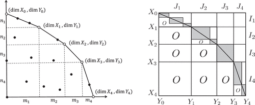
For $(X,Y),(X^{\prime },Y^{\prime })\in {\mathcal{E}}_A$, if $\dim \hspace{0.17em}X\le \dim \hspace{0.17em}{X}^{\prime }$ and $\dim \hspace{0.17em}Y\ge \dim \hspace{0.17em}{Y}^{\prime }$, then $X\subseteq X^{\prime }$ and $Y\supseteq Y^{\prime }$. In particular, ${\mathcal{E}}_A$ is a finite set, and $\varphi$ is injective on ${\mathcal{E}}_A$.

Proof.

We may suppose that $\varphi (X,Y)$ and $\varphi (X^{\prime },Y^{\prime })$ are equal or on an adjacent pair of extreme points. Observe $(X\cap X^{\prime },Y+Y^{\prime }),(X+X^{\prime },Y\cap Y^{\prime })\in {\mathcal{S}}_A$. By the dimension identity of vector spaces, it holds that

$$\varphi (X\cap X^{\prime },Y+Y^{\prime })+\varphi (X+X^{\prime },Y\cap Y^{\prime })=\varphi (X,Y)+\varphi (X^{\prime },Y^{\prime }).$$(4.24)

We claim that $X^{\prime }=X+X^{\prime }$ and $Y^{\prime }=Y\cap Y^{\prime }$, which implies the statement. Otherwise, by (4.24), $\varphi (X\cap X^{\prime },Y+Y^{\prime })$ or $\varphi (X+X^{\prime },Y\cap Y^{\prime })$ goes beyond $\text{Conv}\varphi ({\mathcal{S}}_A)$, which contradicts $(X\cap X^{\prime },Y+Y^{\prime }),(X+X^{\prime },Y\cap Y^{\prime })\in {\mathcal{S}}_A$. □

Therefore, ${\mathcal{E}}_A={\{(X_{\alpha },Y_{\alpha })\}}_{\alpha =0}^{\theta }$ can be arranged as

where ${\mathbb{C}}^n\ne X_1$ and $Y_{\theta -1}\ne {\mathbb{C}}^m$ follow from the assumption that the common left and right kernels of A are trivial. For each $\alpha \in [\theta ]$, let ${\mathcal{L}}_A^{\alpha }$ denote the subset consisting of $(X,Y)\in {\mathcal{S}}_A$ such that $\varphi (X,Y)$ belongs to the edge between $\varphi (X_{\alpha -1},Y_{\alpha -1})$ and $\varphi (X_{\alpha },Y_{\alpha })$. As in the proof of Lemma 4.22, we have:

Lemma 4.23.

If $(X,Y),(X^{\prime },Y^{\prime })\in {\mathcal{L}}_A^{\alpha }$, then $(X+X^{\prime },Y\cap Y^{\prime }),(X\cap X^{\prime },Y+Y^{\prime })\in {\mathcal{L}}_A^{\alpha }$. In particular, ${\mathcal{L}}_A^{\alpha }$ is a modular lattice with respect to the partial order $(X,Y)⪯(X^{\prime },Y^{\prime })\iff X\supseteq X^{\prime },Y\subseteq Y^{\prime }$, where the minimum and maximum elements are given by $(X_{\alpha -1},Y_{\alpha -1})$ and $(X_{\alpha },Y_{\alpha })$, respectively.

For each $\alpha \in [\theta ]$, consider a maximal chain (flag) of ${\mathcal{L}}_A^{\alpha }$:

where the length ${\theta }_{\alpha }$ of the chain is uniquely determined by the Jordan-Dedekind chain condition. The union ${\cup }_{\alpha =1}^{\theta }{\cup }_{\beta =0}^{{\theta }_{\alpha }}\{(X_{\alpha ,\beta },Y_{\alpha ,\beta })\}$ is a maximal chain of the whole lattice ${\mathcal{L}}_A≔{\cup }_{\alpha =1}^{\theta }{\mathcal{L}}_A^{\alpha }$, and is called a DM-flag. Its subset ${\mathcal{E}}_A$ is called the coarse DM-flag, which is uniquely determined by A. From a DM-flag, we obtain a simultaneous block-upper-triangular form of A as follows. Consider $g\in G{L}_n$ including, as row vectors, a basis of $X_{\alpha ,\beta }$ for each $\alpha ,\beta$. Similarly, consider $h\in G{L}_m$ including, as row vectors, a basis of $Y_{\alpha ,\beta }$ for each $\alpha ,\beta$. Suppose that they are positioned in the last rows for g and first rows for h. Then, the matrices $B_{\mathcal{\ell }}=g{A}_{\mathcal{\ell }}{h}^{†}$ are simultaneously block-triangularized, as in the right of Figure 1. We call $B=(B_{\mathcal{\ell }})$ a DM-decomposition⁶ of A. When g (resp. h) is restricted to span only $X_{\alpha }$ (resp. $Y_{\alpha }$), it is called a coarse DM-decomposition of A.

For abuse of notation, $X_{\alpha }$, $X_{\alpha ,\beta }$, $Y_{\alpha }$, and $Y_{\alpha ,\beta }$ also denote the index sets of the corresponding rows and columns of B. Define ordered partitions $(I_{\alpha })$ of [n], $(J_{\alpha })$ of [m], and their refinements $(I_{\alpha ,\beta })$, $(J_{\alpha ,\beta })$ by

Let $\widehat{B}=({\widehat{B}}_{\mathcal{\ell }})$ denote the matrix tuple of block-diagonal matrices obtained from $B_{\mathcal{\ell }}$ by replacing each (upper) off-diagonal block $B_k[I_{\alpha ,\beta },J_{{\alpha }^{\prime },{\beta }^{\prime }}]$ $((\alpha ,\beta )\ne ({\alpha }^{\prime },{\beta }^{\prime }))$ with the zero matrix. We call $\widehat{B}$ a diagonalized DM-decomposition of A. A diagonalized version of a coarse DM-decomposition is defined analogously.

Let $n_{\alpha }≔|I_{\alpha }|$ and $m_{\alpha }≔|J_{\alpha }|$. By convexity of $\text{Conv}\varphi ({\mathcal{S}}_A)$, it holds that

Define $(p^{*},q^{*})\in {\mathbb{R}}^n\times {\mathbb{R}}^m$ by

where the constant $C_A$ is defined bywhere the inequality is seen from the concavity of the harmonic mean $(x,y)\mapsto 2{(1/x+1/y)}^{-1}$. We see from (4.28)–(4.30) that $(p^{*},q^{*})$ belongs to the positive Weyl chamber:

Recalling $P_n^1≔P_n\cap S{L}_n$, define $(G^{*},H^{*})\in {\mathfrak{p}}_n^1\times {\mathfrak{p}}_m^1=T_{I,I}(P_n^1\times P_m^1)$ by

where ${\sigma }^{*}$ is a unitary matrix having a basis of $X_{\alpha }$ in the last $n_{\alpha }$ rows and ${\tau }^{*}$ is a unitary matrix having a basis of $Y_{\alpha }$ in the first $m_{\alpha }$ rows. By using these notions, we give a solution to Problem 4.21 parts (A) and (B):

Theorem 4.24.

• (1) $(p^{*},q^{*})$ is the minimum-norm point of ${\mathit{\Delta }}_A$, and

• (2) $(G^{*},H^{*})/\Vert (G^{*},H^{*})\Vert$ is the unique minimizer of $f_A^{\infty }$ over $S_{I,I}(P_n^1\times P_m^1)$, where it holds that

  $$\Vert (p^{*},q^{*}){\Vert }^2=-f_A^{\infty }(G^{*},H^{*})=\frac{1}{C_A}-\frac{1}{n}-\frac{1}{m}.$$(4.33)

Corollary 4.25.

Let $(g_k,h_k)$ and $(x_k,y_k)$ be the sequences in (4.23) and (4.22), respectively.

• (1) $\text{spec}\mu (g_{k}A{h}_k^{†})$ converges to $(p^{*},q^{*})$ for $k\to \infty$.

• (2) $(x_k,y_k)$ converges, in cone topology, to $(G^{*},H^{*})/\Vert (G^{*},H^{*})\Vert$. More precisely, the sequence $(G_k,H_k)$ defined by $(x_k,y_k)=(e^{t{G}_k/L},e^{t{H}_k/L})$ converges to $(G^{*},H^{*})$ for $k\to \infty$.

Proof of Theorem 4.24.

We first show (4.33). From the definitions of $(p^{*},q^{*})$ and $C_A$, we have

$$\Vert (p^{*},q^{*})+(\mathbf{1}/n,\mathbf{1}/m){\Vert }^2=\frac{1}{C_A^2}{\displaystyle \sum _{\alpha =1}^{\theta }\frac{n_{\alpha }{m}_{\alpha }^2}{{(n_{\alpha }+m_{\alpha })}^2}}+\frac{m_{\alpha }{n}_{\alpha }^2}{{(n_{\alpha }+m_{\alpha })}^2}=\frac{1}{C_A^2}{\displaystyle \sum _{\alpha =1}^{\theta }\frac{n_{\alpha }{m}_{\alpha }}{n_{\alpha }+m_{\alpha }}}=\frac{1}{C_A}.$$

By the last equation in (4.31), we have

$$\Vert (p^{*},q^{*}){\Vert }^2=\Vert (p^{*},q^{*})+(\mathbf{1}/n,\mathbf{1}/m){\Vert }^2-\Vert (\mathbf{1}/n,\mathbf{1}/m){\Vert }^2=1/C_A-1/n-1/m\hspace{0.17em}(>0).$$

On the other hand, $B={\sigma }^{*}A{({\tau }^{*})}^{†}$ is a coarse DM-decomposition, that is, ${({\sigma }^{*}{A}_{\mathcal{\ell }}{({\tau }^{*})}^{†})}_{ij}=0$ for each $(i,j)\in I_{\alpha }\times J_{{\alpha }^{\prime }}$ with $\alpha >{\alpha }^{\prime }$. By (4.21) in the proof of Theorem 4.20, the value of the recession function $f_A^{\infty }(G^{*},H^{*})$ is given by

$$f_A^{\infty }(G^{*},H^{*})=\max \{-p_i^{*}-q_j^{*}\mid \exists \mathcal{\ell },(i,j)\in I_{\alpha }\times J_{{\alpha }^{\prime }}:\alpha \le {\alpha }^{\prime },{({\sigma }^{*}{A}_{\mathcal{\ell }}{({\tau }^{*})}^{†})}_{ij}\ne 0\}.$$(4.34)

Observe from (4.28)–(4.30) that

$$-p_i^{*}-q_j^{*}\{\begin{array}{ll}=1/n+1/m-1/C_A\hfill & \text{if}\hspace{0.17em}(i,j)\in I_{\alpha }\times J_{\alpha },\hfill \\ <1/n+1/m-1/C_A\hfill & \text{if}\hspace{0.17em}(i,j)\in I_{\alpha }\times J_{{\alpha }^{\prime }}:\alpha <{\alpha }^{\prime },\hfill \\ >1/n+1/m-1/C_A\hfill & \text{if}\hspace{0.17em}(i,j)\in I_{\alpha }\times J_{{\alpha }^{\prime }}:\alpha >{\alpha }^{\prime }.\hfill \end{array}$$(4.35)

Hence, the maximum in (4.34) is attained by the index of any nonzero element of any diagonal block of ${\sigma }^{*}{A}_{\mathcal{\ell }}{({\tau }^{*})}^{†}$, which implies $f_A^{\infty }(G^{*},H^{*})=1/n+1/m-1/C_A$, and (4.33).

To complete the proof, it suffices to show $(p^{*},q^{*})\in {\mathit{\Delta }}_A$ because $(p^{*},q^{*})$ and $(G^{*},H^{*})/\Vert (G^{*},H^{*})\Vert$ would attain ${\inf }_{(p,q)\in {\mathit{\Delta }}_A}\Vert (p,q)\Vert ={\sup }_{(G,H)\in B_{I,I}}-f_A^{\infty }(G,H)$. This is done in the next proposition. □

Proposition 4.26.

Let $\widehat{B}$ be a diagonalized DM-decomposition of A.

• (1) $\widehat{B}$ is exactly $(p^{*}+1/n,q^{*}+1/m)$ -scalable.

• (2) $[\widehat{B}]\in \overline{[S{L}_n·A·S{L}_m]}$.

In particular, it holds that $(p^{*},q^{*})\in {\mathit{\Delta }}_A$.

Proof.

Part (1). We first show:

Claim. $B[I_{\alpha ,\beta },J_{\alpha ,\beta }]$ is exactly $(1/|I_{\alpha ,\beta }|,1/|J_{\alpha ,\beta }|)$-scalable.

Proof of Claim.

We can assume that A is already equal to a DM-decomposition B, where all $X_{\alpha ,\beta }$, $Y_{\alpha ,\beta }$ are coordinate subspaces. Suppose indirectly that $B[I_{\alpha ,\beta },J_{\alpha ,\beta }]$ is not exactly $(1/|I_{\alpha ,\beta }|,1/|J_{\alpha ,\beta }|)$-scalable. Then, by Theorem 4.18, there is nontrivial $(Z,W)\in {\mathcal{S}}_{B[I_{\alpha ,\beta },J_{\alpha ,\beta }]}$ such that $(1/|I_{\alpha ,\beta }|)\dim \hspace{0.17em}Z+(1/|J_{\alpha ,\beta }|)\dim \hspace{0.17em}W\ge 1$. Then $(X_{\alpha ,\beta }+Z,Y_{\alpha ,\beta -1}+W)$ belongs to ${\mathcal{S}}_A$. However, $\varphi (X_{\alpha ,\beta }+Z,Y_{\alpha ,\beta -1}+W)$ goes beyond $\text{Conv}\varphi ({\mathcal{S}}_A)$ or lies on the interior of the segment between $\varphi (X_{\alpha ,\beta -1},Y_{\alpha ,\beta -1})$ and $\varphi (X_{\alpha ,\beta },Y_{\alpha ,\beta })$. The former case is obviously impossible. The latter case is also impossible because of the maximality of the chain $\{(X_{\alpha ,\beta },Y_{\alpha ,\beta })\}$ in ${\mathcal{L}}_A$. □

We observe from $n_{\alpha }/m_{\alpha }=|I_{\alpha ,\beta }|/|J_{\alpha ,\beta }|$ that $(m_{\alpha },n_{\alpha })$ is a constant multiple of $(1/|I_{\alpha ,\beta }|,1/|J_{\alpha ,\beta }|)$. By the claim, for each $\alpha ,\beta$, we can choose scaling matrices $g_{\alpha ,\beta },h_{\alpha ,\beta }$ to make $B[I_{\alpha ,\beta },J_{\alpha ,\beta }]$ an exact $(1/\{C_A(n_{\alpha }+m_{\alpha })\})(m_{\alpha }1,n_{\alpha }1)$-scaling. Then, for $g≔{{\displaystyle \oplus }}_{\alpha ,\beta }{g}_{\alpha ,\beta }$, $h≔{{\displaystyle \oplus }}_{\alpha ,\beta }{h}_{\alpha ,\beta }$, the scaling $g\widehat{B}{h}^{†}$ is a desired $(p^{*}+1/n,q^{*}+1/m)$-scaling.

Part (2). Let B be a DM-decomposition of A, where $B\in S{L}_n·A·S{L}_m$. For each $\alpha ,\beta$ and $t>0$, by $B[X_{\alpha ,\beta },Y_{\alpha ,\beta }]=O$, it holds that

Let $R≔{\sum }_{\alpha ,\beta }|X_{\alpha ,\beta }|/n$ and $S≔{\sum }_{\alpha ,\beta }(|Y_{\alpha ,\beta }|-m)/m$. For $t>0$, define $a_t\in S{L}_n$ and $b_t\in S{L}_m$ by

By (4.36), the scaling $a_{t}B{b}_t$ is written as

for the diagonalized DM-decomposition $\widehat{B}$ of B and matrix $E_t$ converging to zero for $t\to \infty$. This implies that ${\lim }_{t\to \infty }[a_{t}B{b}_t]={\lim }_{t\to \infty }[\widehat{B}+E_t]=[\widehat{B}]\in \overline{[S{L}_n·A·S{L}_m]}$. Because $\widehat{B}$ admits an exact $(p^{*}+\mathbf{1}/n,q^{*}+\mathbf{1}/m)$-scaling, $B^{*}=g\widehat{B}{h}^{†}$, by Lemma 4.16 and ${\mathbf{1}}^{\top }{p}^{*}={\mathbf{1}}^{\top }{q}^{*}=0$, we conclude that $(p^{*},q^{*})\in {\mathit{\Delta }}_A$. □

Now the sequence of the scaled matrices along the gradient-descent trajectory accumulates to the $S{U}_n\times S{U}_m$-orbit of a diagonalized DM-decomposition $\widehat{B}$, providing a (partial) solution of Problem 4.21 part (C):

Theorem 4.27.

Let $\widehat{B}$ be a diagonalized DM-decomposition of A, and let $B^{*}$ be a $(p^{*}+\mathbf{1}/n,q^{*}+\mathbf{1}/m)$-scaling of $\widehat{B}$. Then $[g_{k}A{h}_k^{†}]$ accumulates to points in $[S{U}_n·B^{*}·S{U}_m]$ for $k\to \infty$.

Proof.

It holds that $\mu (B^{*})=(\text{diag}\hspace{0.17em}{p}^{*},\text{diag}\hspace{0.17em}{q}^{*})$. Thus, $B^{*}$ attains the infimum of $\Vert \mu (B)\Vert$ over $[B]\in \overline{[S{L}_n·A·S{L}_m]}$, which is also the limit of $\Vert \mu (g_{k}A{h}_k^{†})\Vert$. By the second Ness uniqueness theorem (Theorem 4.15), we have the claim. □

For the gradient flow $(g(t),h(t))$ of the Kempf-Ness function $F_A$ on the group $S{L}_n\times S{L}_m$, because of the convergence theorem (Theorem 4.8), $[g(t)Ah{(t)}^{†}]$ converges to a point $\sigma B^{*}{\tau }^{†}$ for some $\sigma \in S{U}_n$, $s\tau \in S{U}_m$.

Although $B^{*}$ is also a diagonalized DM-decomposition of A, it is not clear how to remove the unitary indeterminacy from $[g_{k}A{h}_k^{†}]$ and to extract the DM-structure of $B^{*}$. This is possible for the coarse DM-structure as follows:

Theorem 4.28.

Let $(G_k,H_k)$ be the sequence defined by $(x_k,y_k)=(e^{k{G}_k/L},e^{k{H}_k/L})$. Suppose that $G_k={\sigma }_k^{†}\text{diag}\hspace{0.17em}{a}^k{\sigma }_k$ and $H_k={\tau }_k^{†}\text{diag}\hspace{0.17em}{b}^k{\tau }_k$ for unitary matrices ${\sigma }_k$, ${\tau }_k$ and nondecreasing and nonincreasing vectors $a^k$ and $b^k$, respectively. Then ${\sigma }_{k}A{\tau }_k^{†}$ accumulates to coarse DM-decompositions. The convergence is linear in the following sense: there are $c>0$, $M>0$ such that for all $k\ge M$, $\mathcal{\ell }\in [N]$ it holds that

$$|{({\sigma }_k{A}_{\mathcal{\ell }}{\tau }_k^{†})}_{ij}|\le e^{-ck}\hspace{1em}((i,j)\in I_{\alpha }\times J_{{\alpha }^{\prime }}:\alpha >{\alpha }^{\prime }).$$

Proof.

By Theorems 3.7 and 4.24 and Lemma 3.9 part (1), it holds that

$$\begin{array}{l}-\frac{1}{L}\left(\frac{1}{C_A}-\frac{1}{n}-\frac{1}{m}\right)=\underset{k\to \infty }{\lim }-\frac{\Vert \nabla f_A(x_k,y_k){\Vert }^2}{L}\hfill \\ =\underset{k\to \infty }{\lim }{f}_A(x_{k+1},y_{k+1})-f_A(x_k,y_k)=\underset{k\to \infty }{\lim }\frac{f_A(x_k,y_k)}{k},\hfill \end{array}$$(4.37)

where the final equality follows from (2.1) for $a_k≔f_A(x_{k+1},y_{k+1})-f_A(x_k,y_k)$.

Because $e^{f_A(x_k,y_k)}=\text{tr}{\sum }_{\mathcal{\ell }}{x}_k{A}_{\mathcal{\ell }}{y}_k{A}_{\mathcal{\ell }}^{†}={\sum }_{\mathcal{\ell },i,j}|{({\sigma }_k{A}_{\mathcal{\ell }}{\tau }_k^{†})}_{ij}{|}^2{e}^{(a_i^k+b_j^k)k/L},$ we have

$${\displaystyle \sum _{\mathcal{\ell },i,j}|}{({\sigma }_k{A}_{\mathcal{\ell }}{\tau }_k^{†})}_{ij}{|}^2{e}^{(a_i^k+b_j^k)k/L-f_A(x_k,y_k)}=1.$$

Suppose that the index $(i,j)$ is in a lower triangular block. By $(a^k,b^k){\to }_{k\to \infty }-(p^{*},q^{*})$ (Corollary 4.25 part (2)) and (4.37), it holds that

$$\frac{(a_i^k+b_j^k)k/L-f_A(x_k,y_k)}{k}\hspace{1em}\underset{k\to \infty }{\to }\hspace{1em}\frac{1}{L}\left(-p_i^{*}-q_j^{*}-\frac{1}{n}-\frac{1}{m}+\frac{1}{C_A}\right)>0,$$

where the inequality follows from (4.35). Therefore, for some $c^{\prime }>0$ and $M^{\prime }>0$, it holds that $(a_i^k+b_j^k)k/L-f_A(x_k,y_k)\ge c^{\prime }k$ for all $k>M^{\prime }$. Then $|{({\sigma }_k{A}_{\mathcal{\ell }}{\tau }_k^{†})}_{ij}{|}^2{e}^{c^{\prime }k}\le 1$ for all $k\ge M^{\prime }$. □

Remark 4.29.

Suppose that $\mu (x_k^{1/2}A{y}_k^{1/2})$ converges, or more strongly, the convergence of Question 3.12 is true. Then it holds that ${\lim }_{k\to \infty }\Vert \mu (x_k^{1/2}A{y}_k^{1/2})+(G_k,H_k)\Vert =0.$ This implies

$$\underset{k\to \infty }{\lim }\Vert \mu (e^{\text{diag}\hspace{0.17em}{a}^k/2}{\sigma }_{k}A{\tau }_k^{†}{e}^{\text{diag}\hspace{0.17em}{b}^k/2})+(\text{diag}\hspace{0.17em}{a}^k,\text{diag}\hspace{0.17em}{b}^k)\Vert =0.$$(4.38)

Because $(a^k,b^k)\to -(p^{*},q^{*})$, the scaling sequence $A^{(k)}≔(e^{\text{diag}\hspace{0.17em}{a}^k/2}{\sigma }_{k}A{\tau }_k^{†}{e}^{\text{diag}\hspace{0.17em}{b}^k/2})/\Vert g_{k}A{h}_k\Vert$ accumulates to $(p^{*}+\mathbf{1}/n,q^{*}+\mathbf{1}/m)$-scalings. From the coarse DM-structure of ${\sigma }_{k}A{\tau }_k^{†}$ in the limit, one can see that $A^{(k)}$ accumulates to diagonalized coarse DM-decompositions. Although our numerical experiment supports such convergence, our results imply only ${\text{lim\hspace{0.17em}inf}}_{k\to \infty }=0$ in (4.38).

We end this subsection with some implications of these results.

4.2.1. On Finding a Destabilizing 1-PSG.

Suppose that A is not $(\mathbf{1}/n,\mathbf{1}/m)$-scalable. Consider $(X^{*},Y^{*})\in {\mathcal{E}}_A$ mapped to the extreme point $(r^{*},s^{*})$ of $\text{Conv}\varphi ({\mathcal{S}}_A)$ with the property that it maximizes r among all extreme points $(r,s)$ maximizing $r+s$. The subspace pair $(X^{*},Y^{*})$ violates (iii) in Theorem 4.17 and is a special certificate of unscalability, called dominant in Franks et al. [19]. By Theorem 4.28, after a large number k of iterations, the last $r^{*}$ rows of ${\sigma }_k$ and the first $s^{*}$ rows of ${\tau }_k$ become bases of an $ϵ$ -approximate dominant pair $(X_{ϵ}^{*},Y_{ϵ}^{*})$ in the sense that $|u^{\top }{A}_{\mathcal{\ell }}\overline{v}|\le ϵ$ for all $\mathcal{\ell }$ and all unit vectors $u\in X_{ϵ}^{*},v\in Y_{ϵ}^{*}$. Franks et al. [19] devised a procedure to round such an $e^{-p(n,m,N,b)}$-approximate dominant pair into the exact dominant pair $(X^{*},Y^{*})$, where p is a polynomial and b is the bit complexity of A. Hence, if we would establish global linear convergence in Theorem 4.28, a polynomial number of iterations of Gradient Descent (4.22) would suffice to recover the dominant pair and a destabilizing 1-PSG.

4.2.2. Matrix Scaling Case.

An $n\times m$ matrix $M=(a_{ij})$ is viewed as a matrix tuple $A={(a_{ij}{e}_i{e}_j^{\top })}_{ij:a_{ij}\ne 0}$. Consider the left-right action on A, in which the group is restricted to the subgroup $S{T}_n\times S{T}_m\subseteq S{L}_n\times S{L}_m$ consisting of diagonal matrices. The corresponding scaling problem is nothing but the matrix scaling problem of the nonnegative matrix $(|a_{ij}{|}^2)$; see Section 3.3. The above results are also applicable to this setting. Indeed, the gradient $\nabla f_A$ is a pair of diagonal matrices. Then, the gradient flow/descent belongs to the diagonal subspace in $P_n^1\times P_m^1$, and is viewed as the gradient flow/descent for the geometric programming objective (3.36) in matrix scaling. Here, all subspaces $X_{\alpha },Y_{\alpha },X_{\alpha ,\beta },Y_{\alpha ,\beta }$ are coordinate subspaces. Hence, a DM-decomposition B is obtained by row and column permutations, and is equivalent to the original (extended) DM-decomposition of M. In Remark 4.29, the unitary matrices ${\sigma }_k$ and ${\tau }_k$ are permutation matrices, and all lower triangular blocks of $A^{(k)}$ become zero matrices after finitely many iterations. Also, all upper triangular blocks of $A^{(k)}$ converge to zero matrices. In particular, the expected convergence to the diagonalized DM-decomposition $\widehat{B}$ is true. This convergence property is almost the same as the one for the Sinkhorn algorithm. Indeed, Hayashi et al. [29] showed that this limit (Sinkhorn limit) oscillates between the $(\mathbf{1},{\sum }_{\alpha }(n_{\alpha }/m_{\alpha }){\mathbf{1}}_{J_{\alpha }})$-scaling $B_{\text{r}}^{*}$ and $({\sum }_{\alpha }(m_{\alpha }/n_{\alpha }){\mathbf{1}}_{I_{\alpha }},\mathbf{1})$-scaling $B_{\text{c}}^{*}$ of $\widehat{B}$.

4.2.3. On the Limit of the Operator Sinkhorn Algorithm.

This suggests an expectation of the limiting behavior of the operator Sinkhorn algorithm (Gurvits’ algorithm), the standard algorithm for the operator scaling problem. The operator Sinkhorn algorithm is viewed as alternating minimization of $f_A(x,y)$, where each step scales $A\to gA$ with $\mu (A)=(O,\ast )$ and $A\to A{h}^{†}$ with $\mu (A)=(\ast ,O)$ alternatively. When it is applied to the $(p^{*}+\mathbf{1}/n,q^{*}+\mathbf{1}/m)$-scaling $B^{*}$ of a diagonalized DM-decomposition $\widehat{B}$, the resulting scaling sequence oscillates between the $(\mathbf{1},{\sum }_{\alpha }(n_{\alpha }/m_{\alpha }){\mathbf{1}}_{J_{\alpha }})$-scaling and $({\sum }_{\alpha }(m_{\alpha }/n_{\alpha }){\mathbf{1}}_{I_{\alpha }},\mathbf{1})$-scaling of $B^{*}$. With the view of Theorem 4.27 and the matrix scaling case above, it is reasonable to conjecture that it oscillates between orbits $U_n·B_{\text{r}}^{*}·U_m$ and $U_n·B_{\text{c}}^{*}·U_m$, where $B_r^{*}$ (resp. $B_c^{*}$) is a $(\mathbf{1},{\sum }_{\alpha }(n_{\alpha }/m_{\alpha }){\mathbf{1}}_{J_{\alpha }})$-scaling (resp. $({\sum }_{\alpha }(m_{\alpha }/n_{\alpha }){\mathbf{1}}_{I_{\alpha }},\mathbf{1})$-scaling) of $\widehat{B}$.

4.3. Kronecker Form of a Matrix Pencil

Finally, we discuss the special case of $N=2$, that is, $A=(A_1,A_2)$. In this case, A is naturally identified with a matrix pencil $s{A}_1+A_2\in \mathbb{C}{(s)}^{n\times m}$, where s is an indeterminate. Here we reveal a connection to the Kronecker canonical form of $s{A}_1+A_2$, and suggest a new numerical method for finding the Kronecker structure based on gradient descent.

A pencil $s{A}_1+A_2$ is called regular if $n=m$ and $\det (s{A}_1+A_2)\ne 0$ for some $s\in \mathbb{C}$. Otherwise, $s{A}_1+A_2$ is called singular. For simplicity, we assume (again) that $\ker \hspace{0.17em}{A}_1\cap \ker \hspace{0.17em}{A}_2=\{0\}$ and $\ker \hspace{0.17em}{A}_1^{†}\cap \ker \hspace{0.17em}{A}_2^{†}=\{0\}$. The Kronecker form is a canonical form of a (singular) pencil under transformation $(s{A}_1+A_2)\to g(s{A}_1+A_2)h^{†}$ by $g\in G{L}_n$, $h\in G{L}_m$. The standard reference of the Kronecker form is Gantmacher [20, chapter XII]; see also Murota [48, section 5.1.3] for its importance in systems analysis. For a positive integer $ϵ$, define $ϵ\times (ϵ+1)$ matrix $L_{ϵ}$ by

Theorem 4.30

(Kronecker Form; Gantmacher [20, Chapter XII]). There are $g\in G{L}_n,h\in G{L}_m$ such that

$$g(s{A}_1+A_2)h^{†}=L_{{ϵ}_1}\oplus L_{{ϵ}_2}\oplus \cdots \oplus L_{{ϵ}_c}\oplus (sC+D)\oplus L_{{\eta }_d}^{†}\oplus L_{{\eta }_{d-1}}^{†}\oplus \cdots \oplus L_{{\eta }_1}^{†},$$(4.39)

where $sC+D$ is a regular pencil, and ${ϵ}_1,{ϵ}_2,\dots ,{ϵ}_c$, ${\eta }_1,{\eta }_2,\dots ,{\eta }_d$ are positive integers determined as follows:

• ${ϵ}_j$ is the minimum degree of a polynomial vector $x_j(s)$ in $\ker \hspace{0.17em}s{A}_1+A_2$ that is linearly independent from $x_1(s),x_2(s),\dots ,x_{j-1}(s)$ over $\mathbb{C}(s)$.

• ${\eta }_j$ is the minimum degree of a polynomial vector $y_j(s)$ in $\ker {(s{A}_1+A_2)}^{†}$ that is linearly independent from $y_1(s),y_2(s),\dots ,y_{j-1}(s)$ over $\mathbb{C}(s)$.

The indices ${ϵ}_1\le \cdots \le {ϵ}_c,{\eta }_1\le \cdots \le {\eta }_d$, called the minimal indices, are uniquely determined. If $n=m$ and $s{A}_1+A_2$ is singular, then the Kronecker form has a zero block with the sum of row and column numbers greater than n. Therefore, by Theorem 4.17, we have:

Corollary 4.31.

A pencil $s{A}_1+A_2$ is regular if and only if $n=m$ and $(A_1,A_2)$ is $(\mathbf{1}/n,\mathbf{1}/n)$-scalable.

We point out a further connection that the Kronecker form (4.39) is viewed as almost a DM-decomposition. Let b denote the number of diagonal blocks of $gA{h}^{†}$ in (4.39). For $\gamma \in [b]$, let $I_{\gamma }$ and $J_{\gamma }$ denote the row and column index sets, respectively, of the $\gamma$-th diagonal block of $gA{h}^{†}$. Define $X_{\gamma }$ by the vector subspace spanned by the rows of g of indices in $I_{\gamma +1}\cup I_{\gamma +2}\cup \cdots \cup I_b$. Similarly, define $Y_{\gamma }$ by the vector subspace spanned by the rows of h having indices in $J_1\cup \cdots \cup J_{\gamma }$. We let $(X_0,Y_0)≔({\mathbb{C}}^n,\{0\})$ (and $(X_b,Y_b)=(\{0\},{\mathbb{C}}^m))$. Suppose that $sC+D(=g(s{A}_1+A_2)h^{†}[I_{c+1},J_{c+1}])$ exists and is an $n_0\times n_0$ upper triangular matrix. Let $Z_{\beta }$ denote the vector space spanned by the rows of g having the last $n_0-\beta$ indices in $I_{c+1}$, and let $W_{\beta }$ denote the vector space spanned by the rows of h having the first $\beta$ indices in $J_{c+1}$. Let $X_{c,\beta }≔X_{c+1}+Z_{\beta }$ and $Y_{c,\beta }≔Y_c+W_{\beta }$, where + is the direct sum. Consider all indices $\gamma$ with $(|I_{\gamma }|,|J_{\gamma }|)\ne (|I_{\gamma +1}|,|J_{\gamma +1}|)$, and suppose that they are ordered as $0≕{\gamma }_0<{\gamma }_1<\cdots <{\gamma }_{\theta }≔b$.

Proposition 4.32.

• (1) ${\{(X_{{\gamma }_{\alpha }},Y_{{\gamma }_{\alpha }})\}}_{\alpha =0}^{\theta }$ is the coarse DM-flag of $(A_1,A_2)$.

• (2) Suppose that $sC+D$ is an $n_0\times n_0$ upper triangular pencil. Then the union of ${\{(X_{\gamma },Y_{\gamma })\}}_{\gamma =0}^b$ and ${\{(X_{c,\beta },Y_{c,\beta })\}}_{\beta =1}^{n_0-1}$ is a DM-flag of $(A_1,A_2)$.

Proof.

Part (1). Suppose that ${\mathcal{E}}_A$ consists of $(X_{\alpha }^{\prime },Y_{\alpha }^{\prime })$ for $\alpha =0,1,2\dots ,{\theta }^{\prime }$, arranged as in (4.25). We show $(X_{\alpha }^{\prime },Y_{\alpha }^{\prime })=(X_{{\gamma }_{\alpha }},Y_{{\gamma }_{\alpha }})$ for $\alpha =0,1,2\dots ,{\theta }^{\prime }=\theta$. Consider the convex hull $K_A$ of $(0,0)$ and $\varphi (X_{\gamma },Y_{\gamma })$ for all $\gamma$. Then $K_A$ belongs to $\text{Conv}\varphi ({\mathcal{S}}_A)$, and the maximal faces of $K_A$ are composed of the line segments connecting points $\varphi (X_{\gamma },Y_{\gamma })$ from $\gamma =0$ to b with bending points $\varphi (X_{{\gamma }_{\alpha }},Y_{{\gamma }_{\alpha }})$.

We show $K_A=\text{Conv}\varphi ({\mathcal{S}}_A)$ by induction on the number b of diagonal blocks. Consider the base case $b=1$ where the Kronecker form consists of a single block. It suffices to show that ${\mathcal{E}}_A=\{({\mathbb{C}}^n,0),(0,{\mathbb{C}}^m)\}$. Suppose that $s{A}_1+A_2$ is an $n_0\times n_0$ regular pencil $sC+D$. By regularity, there is no $(X,Y)\in {\mathcal{S}}_A$ with $\dim \hspace{0.17em}X+\dim \hspace{0.17em}Y>n_0$ (otherwise $s{A}_1+A_2$ is singular over $\mathbb{C}(s)$). This means no point in $\varphi ({\mathcal{S}}_A)$ beyond the line segment between $(n_0,0)$ and $(0,n_0)$. Therefore, we have ${\mathcal{E}}_A=\{({\mathbb{C}}^n,0),(0,{\mathbb{C}}^m)\}$. Suppose that $s{A}_1+A_2=L_n$. Suppose to the contrary that there is $(X,Y)\in {\mathcal{S}}_A$ with $\dim \hspace{0.17em}X/n+\dim \hspace{0.17em}Y/(n+1)>1$. By basis change, we may assume that

$$s{A}_1+A_2=\left(\begin{array}{cc}B& C\\ O& D\end{array}\right),$$

where O is the $r\times s$ zero matrix for $(r,s)≔(\dim \hspace{0.17em}X,\dim \hspace{0.17em}Y)$. By $r\ge 1$ and $r+s\ge n+1$, B is a pencil of $n-r$ rows and s columns with $s>n-r$. Then $\ker \hspace{0.17em}B$ contains a polynomial vector with degree at most $n-r<n$; use Cramer’s formula to see this. Necessarily, $\ker \hspace{0.17em}s{A}_1+A_2$ also has such a polynomial vector. This is a contradiction to Theorem 4.30 (${ϵ}_1={ϵ}_c=n$). The case $s{A}_1+A_2=L_n^{†}$ is similar.

Consider a general case of $b\ge 2$. We can choose ${\gamma }^{*},{\alpha }^{*}$ such that $0<{\gamma }^{*}<b$, $0<{\alpha }^{*}<{\theta }^{\prime }$, and the line segment between $\varphi (X_{{\gamma }^{*}},Y_{{\gamma }^{*}})$ and $\varphi (X_{{\alpha }^{*}}^{\prime },Y_{{\alpha }^{*}}^{\prime })$ meets with $K_A$ only at $\varphi (X_{{\gamma }^{*}},Y_{{\gamma }^{*}})$. Consider $(U,V)≔(X_{{\gamma }^{*}}+X_{{\alpha }^{*}}^{\prime },Y_{{\gamma }^{*}}\cap Y_{{\alpha }^{*}}^{\prime })$ and $(U^{\prime },V^{\prime })≔(X_{{\gamma }^{*}}\cap X_{{\alpha }^{*}}^{\prime },Y_{{\gamma }^{*}}+Y_{{\alpha }^{*}}^{\prime })$. By the construction and (4.24), one of $\varphi (U,V)$ and $\varphi (U^{\prime },V^{\prime })$ is outside of $K_A$. Suppose that $\varphi (U,V)\notin K_A$. Consider the submatrix $A^{\prime }≔(s{A}_1+A_2)[{\cup }_{\gamma =1}^{{\gamma }^{*}}{I}_{\gamma },{\cup }_{\gamma =1}^{{\gamma }^{*}}{J}_{\gamma }]$, which is also a Kronecker form with a smaller number of blocks. From $U\supseteq X_{{\gamma }^{*}}$, $V\subseteq Y_{{\gamma }^{*}}$, and $\varphi (U,V)\notin K_A$, it necessarily holds that $K_{A^{\prime }}\ne \text{Conv}\varphi ({\mathcal{S}}_{A^{\prime }})$. However, this is a contradiction to the inductive assumption. The case $\varphi (U^{\prime },V^{\prime })\notin K_A$ is similar; consider the sub-Kronecker form $(s{A}_1+A_2)[{\cup }_{\gamma ={\gamma }^{*}+1}^b{I}_{\gamma },{\cup }_{\gamma ={\gamma }^{*}+1}^b{J}_{\gamma }]$.

Part (2). Observe that all integer points in the maximal faces of $\text{Conv}\varphi ({\mathcal{S}}_A)$ are obtained by the images of $(X_{\gamma },Y_{\gamma })$ and $(X_{c,\beta },Y_{c,\beta })$. This implies that ${\{(X_{\gamma },Y_{\gamma })\}}_{\gamma }\cup {\{(X_{c,\beta },Y_{c,\beta })\}}_{\beta }$ is a maximal chain of ${\mathcal{L}}_A$. □

The matrix pencil $g(s{A}_1+A_2)h^{†}$ corresponding to a coarse DM-decomposition $g(A_1,A_2)h^{†}$, which we call a coarse Kronecker triangular form, is a refinement of a quasi-Kronecker triangular form in Berger and Trenn [7] and generalized Schur form in Demmel and Kåragström [16] and Van Dooren [59] if g, h are unitary matrices and $sC+D$ is triangular.

Then, the convergence (Theorem 4.28) of Gradient Descent (4.22) can be applied as follows:

Theorem 4.33

(Convergence to a Coarse Kronecker Triangular Form). Let $(x_k,y_k)$ be a solution of (4.22). Decompose $x_k={\sigma }_k^{†}{e}^{\text{diag}\hspace{0.17em}{a}^k}{\sigma }_k$ and $y_k={\tau }_k^{†}{e}^{\text{diag}\hspace{0.17em}{b}^k}{\tau }_k$, where ${\sigma }_k$ and ${\tau }_k$ are unitary matrices, and $a^k$ and $b^k$ are nondecreasing and nonincreasing vectors, respectively. Then, ${\sigma }_k(s{A}_1+A_2){\tau }_k^{†}$ accumulates to coarse Kronecker triangular forms, where the convergence is linear in the same sense as in Theorem 4.28.

A coarse Kronecker triangular form is enough for determining the structure of the Kronecker form. Indeed, each (nonsquare) rectangular diagonal block is a $k\nu \times k(\nu +1)$ or $k(\nu +1)\times k\nu$ matrix for some integers $k,\nu$, from which all minimal indices ${ϵ}_1,{ϵ}_2,\dots ,{ϵ}_c$, ${\eta }_1,{\eta }_2,\dots ,{\eta }_d$ can be identified.

The above theorem suggests an iterative method for determining the minimal indices of a singular pencil, which is based on simple gradient descent and is conceptually different from the existing algorithms, for example, Demmel and Kåragström [16] and Van Dooren [59]. It is an interesting future direction to develop a numerically stable algorithm based on this approach.

References

- [1] (2018) Operator scaling via geodesically convex optimization, invariant theory and polynomial identity testing. Diakonikolas I, Kempe D, eds. Proc. 50th Annual ACM SIGACT Sympos. Theory Comput. STOC 2018 (Association for Computing Machinery, New York), 172–181.Google Scholar
- [2] (2004) Hessian Riemannian gradient flows in convex programming. SIAM J. Control Optim. 43(2):477–501.Crossref, Google Scholar
- [3] (2008) Gradient Flows: In Metric Spaces and in the Space of Probability Measures, 2nd ed. (Birkhäuser, Basel, Switzerland).Google Scholar
- [4] (1997) How to deal with the unbounded in optimization: Theory and algorithms. Math. Programming 79(1–3):3–18.Crossref, Google Scholar
- [5] (2014) Convex Analysis and Optimization in Hadamard Spaces (De Gruyter, Berlin).Crossref, Google Scholar
- [6] (2017) First-Order Methods in Optimization (Society for Industrial and Applied Mathematics, Philadelphia).Crossref, Google Scholar
- [7] (2012) The quasi-Kronecker form for matrix pencils. SIAM J. Matrix Anal. Appl. 33(2):336–368.Crossref, Google Scholar
- [8] (2023) An Introduction to Optimization on Smooth Manifolds (Cambridge University Press, Cambridge, UK).Crossref, Google Scholar
- [9] (1999) Metric Spaces of Non-Positive Curvature (Springer-Verlag, Berlin).Crossref, Google Scholar
- [10] (2015) Convex optimization: Algorithms and complexity. Foundations Trends Machine Learn. 8(3–4):231–357.Crossref, Google Scholar
- [11] (2020) Interior-point methods for unconstrained geometric programming and scaling problems. Preprint, submitted August 27, https://arxiv.org/abs/2008.12110.Google Scholar
- [12] (2018) Efficient algorithms for tensor scaling, quantum marginals, and moment polytopes. Thorup M, ed. Proc. 59th IEEE Annual Sympos. Foundations Comput. Sci. FOCS 2018 (IEEE, New York), 883–897.Google Scholar
- [13] (2019) Towards a theory of non-commutative optimization: Geodesic 1st and 2nd order methods for moment maps and polytopes. Proc. 60th IEEE Annual Sympos. Foundations Comput. Sci. FOCS 2019 (IEEE, New York), 845–861.Google Scholar
- [14] (2010) At infinity of finite-dimensional CAT(0) spaces. Math. Ann. 346(1):1–21.Crossref, Google Scholar
- [15] (2014) Calabi flow, geodesic rays, and uniqueness of constant scalar curvature Kähler metrics. Ann. Math. 180(2):407–454.Crossref, Google Scholar
- [16] (1993) The generalized Schur decomposition of an arbitrary pencil —Robust software with error bounds and applications. I. Theory and algorithms. ACM Trans. Math. Software 19(2):160–174.Crossref, Google Scholar
- [17] (1958) Coverings of bipartite graphs. Canadian J. Math. 10:517–534.Crossref, Google Scholar
- [18] (2018) Operator scaling with specified marginals. Diakonikolas I, Kempe D, eds. Proc. 50th Annual ACM SIGACT Sympos. Theory Comput. (STOC 2018) (Association for Computing Machinery, New York). 190–203.Google Scholar
- [19] (2023) Shrunk subspaces via operator Sinkhorn iteration. Bansal N, Nagarajan V, eds. Proc. 2023 Annual ACM-SIAM Sympos. Discrete Algorithms (SODA) (SIAM, Philadelphia), 1655–1668.Google Scholar
- [20] (1959) The Theory of Matrices, vol. 1–2 (Chelsea Publishing Co., New York).Google Scholar
- [21] (2018) Recent progress on scaling algorithms and applications. Bull. Eur. Assoc. Theoret. Comput. Sci. (125):14–49.Google Scholar
- [22] (2018) Algorithmic and optimization aspects of Brascamp-Lieb inequalities, via operator scaling. Geometric Funct. Anal. 28(1):100–145.Crossref, Google Scholar
- [23] (2020) Operator scaling: Theory and applications. Foundations Comput. Math. 20(2):223–290.Crossref, Google Scholar
- [24] (2021) The Moment-Weight Inequality and the Hilbert-Mumford Criterion—GIT from the Differential Geometric Viewpoint, Lecture Notes in Mathematics, vol. 2297 (Springer, Cham, Switzerland).Google Scholar
- [25] (1982) Convexity properties of the moment mapping. Inventiones Math. 67(3):491–513.Crossref, Google Scholar
- [26] (1984) Convexity properties of the moment mapping. II. Inventiones Math. 77(3):533–546.Crossref, Google Scholar
- [27] (2004) Classical complexity and quantum entanglement. J. Comput. System Sci. 69(3):448–484.Crossref, Google Scholar
- [28] (2021) Computing the nc-rank via discrete convex optimization on CAT(0) spaces. SIAM J. Appl. Algebra Geometry 5(3):455–478.Crossref, Google Scholar
- [29] (2023) Finding Hall blockers by matrix scaling. Math. Oper. Res. 49(4):2166–2179.Link, Google Scholar
- [30] (2024) Convex analysis on Hadamard spaces and scaling problems. Foundations Comput. Math. 24(6):1979–2016.Crossref, Google Scholar
- [31] (2025) Generalized gradient flows in Hadamard manifolds and convex optimization on entanglement polytopes. Preprint, submitted November 15, https://arxiv.org/abs/2511.12064v1.Google Scholar
- [32] (2026) A scaling characterization of nc-rank via unbounded gradient flow. Linear Algebra Appl. 730:525–545.Crossref, Google Scholar