Frontiers in Operations: You, Me, or We? Coproductive Principal-Agent Dynamics
Abstract
Problem definition: Projects are often initiated by a single person—a principal—who then decides whether to form a team by sharing project value with an agent. We ask the following: When does a principal form a team, and which operating mode emerges in equilibrium—single execution by the principal, delegated execution to the agent, or joint execution? Methodology/results: We consider a coproductive principal-agent model with endogenous team formation. In the second best, joint execution is less frequent than optimal, whereas both single and delegated execution are chosen too much. With a linear contract, common with nonfinancial output (credits, coauthorship) or in entrepreneurial ventures, there is too much single execution; that is, the principal does not form a team often enough, and there is either too little joint execution when one of the workers has low productivity or too little delegation otherwise. Overall, the inefficiency in project execution (due to moral hazard) appears less severe than the inefficiency in the principal’s team formation decision (due to project hoarding). Managerial implications: Managerial under-delegation fundamentally stems from project hoarding; that is, principals do not partner enough. When principals choose to form a team, they then might delegate too much; paradoxically, this happens when agents have low productivity. Although the existing literature focuses on eliciting agent effort for a given operating mode, our analysis suggests the decision to form a team (or not) is a more critical issue.
History: This paper has been accepted in the Manufacturing & Service Operations Management Frontiers in Operations Initiative.
Supplemental Material: The online appendix is available at https://doi.org/10.1287/msom.2025.0016.
1. Introduction
Many projects, be they research or innovation projects, entrepreneurial ventures, or service provisions, are often initiated by a single person—a principal—who then decides whether to form a team by partnering with someone else—an agent—and if so, how to share the project value. Then, depending on the principal’s and the agent’s respective incentives, efforts are exerted simultaneously and noncooperatively, leading to the emergence of one of the following three operating modes: single execution by the principal (SE), delegated execution to the agent (DE), or joint execution (JE). Which operating mode emerges in these coproductive dynamics?
Such coproductive dynamics arise in a variety of settings in operations management (OM). For instance, entrepreneurs often need to decide whether to pursue growing their venture alone or to partner with someone else (Kamm and Nurick 1993, de Bettignies 2008, Yoo et al. 2016), such as venture capitalists (Bergemann and Hege 1998, Casamatta 2003). Innovation projects can be conducted by sole inventors or teams (Wuchty et al. 2007, Kavadias and Sommer 2009, Singh and Fleming 2010, Chan et al. 2021). Services can be executed as self-services, completely outsourced, or coproduced by a service provider and a client (Vargo and Lusch 2004; Roels 2014; Bellos and Kavadias 2019, 2021). Supply chain management involves outsourcing and subcontracting (Van Mieghem 1999, Baiman et al. 2000) and collaborations (Corbett and DeCroix 2001, Corbett et al. 2005, Bhaskaran and Krishnan 2009, Kim and Netessine 2013). Collaboration is also ubiquitous within organizations (Alchian and Demsetz 1972, Bonatti and Hörner 2011) and often arises organically, for example, in self-managed teams (Lee and Edmondson 2017). Coproductive organizational settings are going to be even more salient with the development of agentic artificial intelligence (AI) (Bastani and Cachon 2025, Fügener et al. 2026) with “billions of agents inside of every company, and across every imaginable field.”1 At numerous touchpoints in cross-functional processes, human workers may need to decide how to collaborate with agents equipped with commercial objectives, self-driven marketing, self-fundraising, and self-governance capabilities.2
1.1. Model Setup
We extend in two ways the canonical principal-agent (PA) model with moral hazard, that is, unobservable efforts. First, we allow the principal to contribute to the execution of the project, either with the agent (JE) or alone (SE). Second, we study the genesis of teams by endogenizing the principal’s team formation decision. We refer to the sequential decisions of team formation and effort execution as “coproductive dynamics.”
Our stylized model is characterized by two sources of inefficiency: (i) the single or double moral hazard associated with effort execution within an operating mode, which has been the focus of the PA literature (Holmström 1979) under DE and the team production (TP) literature (Holmström 1982) under JE; and (ii) the lack of control over the principal’s decision to form a team—another form of moral hazard—resulting in a potentially inefficient operating mode.
We characterize the coproductive dynamics in three settings: (i) in the first best (FB), when the objective is to maximize the total value net of the effort costs; (ii) in the second best (SB), when the principal offers a two-part tariff, requiring the agent to pay the principal for the agent’s equity share, as often happens in franchises (Bhattacharyya and Lafontaine 1995), joint ventures (Sampson 2007), and venture capital (Bergemann and Hege 1998, Casamatta 2003); and (iii) when the principal offers a linear (i.e., proportional) output-sharing contract to the agent (e.g., coauthorship, credit on a common project, patent ownership) without receiving a fixed payment in return, with weight assigned depending on prominence or recognition (e.g., first versus second author), as often happens when financial transfers are uncommon or impossible.
1.2. Research Questions
We investigate the following research questions:
How do the coproductive dynamics with a linear contract differ from the FB and SB?
Does the possibility of coproduction always benefit the principal?
What is the most severe source of inefficiency: the moral hazard associated with effort execution or the principal’s endogenous decision to form a team?
1.3. Results
We obtain the following results. First, we compare the equilibrium coproductive dynamics with a linear contract to the FB and SB benchmarks. In the FB, JE is optimal when the degree of effort substitutability is low and the workers have similar productivities. Otherwise, the optimal choice between DE and SE fully relies on allocating work to the most productive party. The SB coproductive dynamics are similar to the FB, with too much SE and DE and too little JE, because only JE is subject to moral hazard. With a linear (i.e., proportional) output-sharing rule, there is too much SE compared with the FB because the principal can create and capture the full value whenever SE is the FB operating mode. There might be too little JE, like in the SB, but this time only when one of the workers has low productivity. Otherwise, there may be too little DE. Also, greater effort substitutability no longer implies less JE, unlike the FB and SB.
Second, we find that the coproductive nature of the task, despite being beneficial in the FB by offering flexibility to shift work to the most productive party, may hurt the principal. In particular, the principal may benefit from having a higher cost of effort, to commit not to engage in JE, thus having more freedom in setting the agent’s incentives under DE. This is reminiscent of the value of commitment in industrial organization (Fudenberg and Tirole 1984) and project selection (Aghion and Tirole 1997).
Finally, we find that the loss associated with the principal’s endogenous team formation—resulting in an inefficient operating mode—can be much more severe than the loss associated with the decentralized effort execution. Specifically, the total value under a linear output-sharing agreement may sharply decline as the degree of effort substitutability increases, unlike the FB and SB total values, which are increasing in it. This drop arises when the principal engages in project hoarding (SE) even if a team is (FB or SB) optimal. Hence, although the PA and TP literatures have focused on incentives in effort execution, the team formation decision appears to be more critical.
In Section EC.2 of the Online Appendix, we consider a setting where the principal can freely commit to an effort level before the agent chooses theirs. The coproductive dynamics turn out to be very similar to the case where efforts are chosen simultaneously, with slightly less project hoarding by the principal. However, the principal benefits in this case from the coproductive nature of the task because they can control whether to engage in JE by committing to their effort before the agent.
1.4. Implications
The problem of managerial under-delegation should really be framed as stemming from project hoarding, that is, principals partnering too little. When they do, they may in fact delegate too much; this arises, paradoxically, when agents exhibit low productivity. Conversely, they may engage too much in joint execution rather than delegating the execution entirely to the agent, when—again counterintuitively—the agent is highly productive. Our model calls for more research on devising mechanisms to entice principals to refrain from hoarding and instead form teams. Our stylized model should serve as a cautionary tale for the development of agentic AI, predicting that human workers may under-use AI agents to retain all the project value for themselves, either financial (e.g., crypto-currency allocated to AI agents) or nonfinancial (recognition). Also, if human workers use AI agents, human-AI collaboration is far from guaranteed, despite the ubiquity of this operating mode in the managerial and management research literatures.
2. Literature Review
We contribute to three interconnected streams of literature: the literature on PA models, the literature on TP, and the literature on task allocation. We conclude this section with an overview of affine and linear contractual arrangements.
2.1. Principal-Agent Models
The PA literature typically assumes that an agent has been hired by a principal to execute a task (Holmström 1979); that is, it implicitly assumes that DE is adopted. PA models have been enhanced in numerous ways, including risk aversion, multiple tasks (Holmström and Milgrom 1991), information asymmetry, and sequential decision making (Winter 2004). PA models have been applied to various OM settings, for example, for supply chain contracting (Cachon 2003). Sticking to a one-task, full-information, risk-neutral case, we take a step back from these models and investigate team genesis in a coproductive setting, allowing the principal to contribute either alone (SE) or jointly with the agent (JE).
2.2. Team Production
TP involves peers contributing to a common output and sharing some equity, resulting in double moral hazard in the absence of a third party who can collect the project’s net surplus without contributing to it, called a “budget breaker” (Holmström 1982, Kim and Wang 1998). In most cases, TP models implicitly assume that JE is adopted. Given the increased prevalence of teamwork in organizations, this stream has recently expanded, studying collaborative dynamics (Siemsen et al. 2007, Bonatti and Hörner 2011, Georgiadis 2014, Georgiadis et al. 2014, Rahmani et al. 2017, Crama et al. 2019) and innovation (Wuchty et al. 2007, Jones 2021, Candoğan et al. 2025) within an organizational context. In addition, research on collaboration or coproduction across organizations has recently thrived, not only in service management (Vargo and Lusch 2004), but also in franchising (Bhattacharyya and Lafontaine 1995), joint ventures (Sampson 2007), entrepreneurship (Bergemann and Hege 1998, Casamatta 2003), supply chains (Corbett and DeCroix 2001, Kim and Netessine 2013), quality management (Baiman et al. 2000), and new product development (Bhaskaran and Krishnan 2009).
We make two contributions to this literature. First, we adopt a generic perspective on value coproduction, demonstrating the robustness of many insights obtained in the literature with more specific value functions, such as additive (Karmarkar and Pitbladdo 1995, Bhaskaran and Krishnan 2009, Yoo et al. 2016, Bellos and Kavadias 2019), multiplicative or Cobb-Douglas (Wang and Zhou 2004, Roels et al. 2010, Kim and Netessine 2013, Crama et al. 2017, Andritsos and Tang 2018), constant elasticity of substitution (CES) (Bhattacharyya and Lafontaine 1995, Roels 2014, Rahmani et al. 2018, Candoğan et al. 2025), and convex combination of minimum and maximum functions (Dong et al. 2025). In our characterization of the equilibrium coproductive dynamics, we consider a more specialized coproductive value function, imported from decision analysis (Keeney and Raiffa 1976), but still generalizing the additive and multiplicative cases among others. Second, and more importantly, we endogenize the team formation decision, which must precede the development of any coproductive relationship.
2.3. Task Allocation
In contrast to the PA and TP models, which focus on effort exertion within an operating mode, other models consider the choice across operating modes, although it is often restricted to a dichotomous selection between SE and DE. In particular, the literature on property rights (Grossman and Hart 1986) studies who, between a principal and an agent, should own a key productive asset. Similarly, the literature on delegation analyzes who should make a critical decision about a project (Aghion and Tirole 1997, Prendergast 2002). In particular, Prendergast (1995) shows analytically that managers tend to delegate too few tasks and spend too much effort on their tasks, whereas agents spend too little effort on theirs. Such task allocation models have been widely studied in OM applications, including outsourcing or subcontracting (Van Mieghem 1999, Bhaskaran and Krishnan 2009), service provision (Bellos and Kavadias 2019, 2021), task delegation by an entrepreneur (Yoo et al. 2016), effort provision in new ventures (de Bettignies 2008), and research and development (R&D) licensing (Xiao and Xu 2012). In multitask extensions of these models, Itoh (2001), Hagiu and Wright (2019), and Bellos and Kavadias (2019, 2021) investigate how to allocate a subset of tasks between a principal and an agent. We differ from the task allocation literature in two ways. First, this literature considers some form of ex ante allocation of property or decision rights, whereas we assume here that workers are free to exert effort or not. Thus, operating modes cannot be enforced, but instead must emerge in equilibrium; in particular, DE may not be achievable if the principal wants to contribute. Second, this literature generally ignores the possibility of JE, limiting the task allocation between DE and SE.
2.4. Affine and Linear Contracts
Both the PA and TP streams of literature consider affine and linear contracts due to their prevalence in practice. In the PA literature, Holmström and Milgrom (1987) show that affine contracts are asymptotically optimal, and Carroll (2015) shows they are robust. Bhattacharyya and Lafontaine (1995) and Kim and Wang (1998) show they are also optimal in a coproductive PA relationship, and Nandeibam (2002) establishes that they naturally emerge in TP. Such affine contracts are indeed common in profit-sharing firms and partnerships as described by Alchian and Demsetz (1972) in their typology of firms.
When fixed-fee transfers are not allowed, linear (i.e., proportional) output-sharing contracts are in general not optimal. However, they are convenient and widely adopted in practice. For instance, Gaynor and Gertler (1995) report their wide adoption in medical group practices. Cachon and Lariviere (2005) study the performance of such “revenue-sharing” contracts in vertical supply chains, whereas Chi (1996) and Marinucci (2009) study the effort dynamics associated with such “equity” contracts in horizontal joint ventures. Linear contracts are common in settings where financial transfers are not allowed (e.g., patent ownership, coauthorship, movie credits), as is common within organizations, similar to Bonatti and Hörner (2011), Georgiadis (2014), and Georgiadis et al. (2014).
3. Model
We first present the game formulation (Section 3.1), then discuss the different roles played by the principal and the agent (Section 3.2), and explain our modeling assumptions (Section 3.3). Finally, Section 3.4 outlines how we model the degree of effort substitutability.
3.1. Game Formulation
The game consists of two stages, depicted in Figure 1. In a team formation stage, the principal chooses whether to partner with an agent, and if so, how to share the project value with them. Then, in an execution stage, efforts are exerted, simultaneously and noncooperatively.
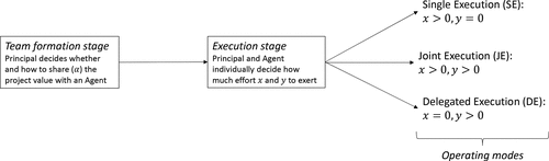
Let x and y denote the principal’s and the agent’s percentage of time commitment to the execution of the project, or effort, lying in [0, 1], and assumed to be unobservable. We have SE if and , DE if and , and JE if and .
Let denote the expected project output, or value, by default fully captured by the principal. Assuming linear costs of effort (without loss of generality, as discussed in Section 3.3.3), let and denote, respectively, the principal’s and the agent’s unit costs of effort.
As a benchmark, consider the problem of maximizing the total net value, which we refer to as the FB solution:
Consider now the decentralized game, restricting our attention to contracts that are either affine (Section 6) or linear (Section 7) in . Let be the principal’s residual share of output. The principal forms a team if and only if . In case of nonfinancial output share, captures the prominence or recognition (e.g., first versus second author); for simplicity, we assume it to be continuous, as is the case for patents (Kaptay 2020) and venture equity. Let f be the fixed transfer payment, positive when it is from the agent to the principal and negative otherwise. Under a linear contract, .
In the team formation stage, the principal chooses the contract that maximizes their payoff, anticipating the equilibrium efforts chosen in the execution stage and subject to the agent’s participation constraint, assuming a null reservation utility:
Because the fixed fee f does not affect the equilibrium efforts, it is omitted in the equilibrium formulation of the execution stage in (3) and (4). In the case of multiple equilibria, the principal is assumed to select the one that they prefer.
The characterization of equilibrium efforts for a given output share will follow a similar characterization as the FB solution, because the FB efforts from (1) with inflated costs and solve (3) and (4). In both cases, we generically refer to SE and DE as “solo” modes and JE as “duo” mode. Accordingly, we will denote by the principal’s solo effort (under SE), by the agent’s solo effort (under DE), and by their respective duo efforts (under JE).
3.2. Roles
What distinguishes the principal from the agent? The principal is the project initiator; for instance, the principal can be at the origin of the idea of the venture, have secured its initial financing, or own a proprietary technology or legal rights. Accordingly, they have a residual claim on its value. As formalized by the property rights literature (Grossman and Hart 1986, Holmström and Milgrom 1994) and the TP literature (Alchian and Demsetz 1972), authority is conferred by the ownership of an asset (e.g., the project idea), which gives the owner the right to make decisions concerning the use of this asset (the right to partner or not and apportion rewards). Accordingly, the principal is responsible for team formation.
Who executes the project emerges as an equilibrium outcome in (3) and (4), which follows from the incentives set in the team formation stage (2). This is in contrast to the PA literature, which implicitly assumes DE under any sharing rule; the TP literature, which assumes JE under any sharing rule; and the task allocation literature, which assumes that principals can choose how to allocate tasks (i.e., between DE and SE) under any sharing rule. This departure from the literature stems from the combination of two factors: the coproductive nature of the value function and the inability, for any party, to commit to any particular effort.3
Under SE, there is role concentration given that the principal is in charge of both the project initiation and its execution. Under DE, there is role specialization given that the principal is in charge of the project initiation and team formation, whereas the agent is in charge of the project execution. Under JE, there is role sharing at the level of the project execution.
3.3. Assumptions
We next introduce some restrictions on the value function and justify some modeling assumptions made in the game formulation presented in Section 3.1.
3.3.1. Value.
The expected value of the project is assumed to be continuously twice differentiable, strictly increasing, and strictly concave in x and y, although not necessarily jointly, for any with either or , which we write as . The value function may not necessarily be symmetric. Let denote the project’s potential value.
To avoid trivial cases, we assume that efforts are strategic substitutes, that is, for all . Indeed, if they were strategic complements, that is, for all , JE would be the only FB operating mode. (The proof is omitted.)
Our characterization of the coproductive dynamics in the FB (Section 4) and SB (Section 6) holds for any generic functional form of that satisfies the above conditions. This includes the following functional form of the value function:
In this functional family, the joint effort is bilinear, which is a functional form commonly used in the decision analysis literature (Keeney and Raiffa 1976, section 5.4.1). It specializes to xy when , when , and when .
Another possible functional form is the CES function (Bhattacharyya and Lafontaine 1995):
In these two examples, the joint effort functions, or , are such that efforts become more substitutable when k increases—a characteristic we will formalize in Section 3.4. Although these two functional families are symmetric, could be asymmetric.
Our characterization of the coproductive dynamics under a linear contract (Section 7) assumes that is given by (6) for tractability. The proofs of the results that consider a generic value function appear in the appendix; the proofs of the results that rely on (6) appear in Section EC.1 of the Online Appendix.
3.3.2. Boundary Conditions.
We assume that and , as well as and , to ensure that the project is undertaken but that workers never find it beneficial to dedicate 100% of their time to it.
3.3.3. Costs of Effort.
With linear costs of effort, their marginal costs at zero are positive, for any . We make this assumption because, if they were zero (e.g., as if effort costs were and with ), JE would be the only FB operating mode (Corbett and DeCroix 2001, Corbett et al. 2005). Under the condition that marginal costs at zero are positive, the assumption of cost linearity is without loss of generality given our abstract representation of .
3.3.4. Uncertainty.
We assume that uncertainty affects the coproductive dynamics only through the project’s expected value . Uncertainty may impact outcomes by affecting the probability of success of a binary outcome (Bonatti and Hörner 2011), for example, for some increasing function with and , or additively, for example, , where is a random noise and is an increasing concave function (Bhattacharyya and Lafontaine 1995, Bhaskaran and Krishnan 2009, Bellos and Kavadias 2021). In the context of supply chain collaboration, may represent the expected sales given inputs x and y and a random demand . In particular, if x and y are perfect substitutes, as it happens with partial subcontracting (Van Mieghem 1999), and if they are perfect complements, as it happens in assembly systems (Gerchak and Wang 2004).
Given the single-period nature of our model, like most seminal PA models (Holmström 1979, 1982; Holmström and Milgrom 1987), we do not capture the effect of uncertainty resolution on belief updates that would be characteristic of a dynamic setting. There is also no private information besides the unobservable efforts and private costs; that is, we focus on moral hazard and leave out the question of adverse selection.
3.3.5. Participation Constraint.
Although we explicitly model the agent’s participation constraint (5), we ignore it in our analysis of the coproductive dynamics under a linear contract (7), which is without loss of optimality when is sufficiently large. For instance, when is given by (6), requiring that
3.4. Degree of Effort Substitutability
We will depict the coproductive dynamics as a function of the value function’s degree of effort substitutability, parameterized with k. For instance, a project may be more structured or less complex, making division of labor more appealing. To formalize this definition, we expand the argument set of to formally express its dependence on k as . (The semicolon separates the decision variables from the parameters.) Similarly, we formalize the potential dependence of the solo efforts and (defined at the end of Section 3.1) on k as and . With this notation, and assuming differentiability, we define parameter k as reducing the marginal return of a worker who does: not exert effort, whereas the other does:
The parameter k in the symmetric functional forms of the joint effort functions (bilinear, CES) presented in Section 3.3.1 satisfies this definition.
4. First-Best Solution
Our first benchmark is the FB solution (1). Because its objective function is continuous and the feasible set is bounded, Weierstrass’s theorem guarantees the existence of an optimal solution, which we denote by .
4.1. Efforts in Each Operating Mode
We consider the following three candidates for local maxima of (1) and specify the conditions under which they satisfy the Karush-Kuhn-Tucker conditions, that is, are critical points:
SE:, in which solves ; it is a critical point if ;
DE:, in which solves ; it is a critical point if ;
JE:, which solves and ; it is a critical point if , and .
The values , , , and are uniquely defined given that is coordinate-wise strictly concave and has a negative cross derivative.4 When is given by (6), (A.1) provides the closed-form expressions of these candidates for local maxima. The boundary conditions in Section 3.3.2 ensure that ; also, (i) if , then , and (ii) if , then . Although the second-order optimality conditions are automatically satisfied at and , if they are critical, they may not be so at , which may just be a saddle point (Lemma B.1) given that is not necessarily jointly concave.
4.2. Which Operating Modes Emerge
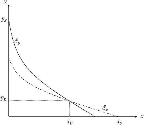
The next proposition characterizes which operating modes emerge in the FB solution in the space, keeping constant, and is illustrated in Figure 2 (right) with a specific example. The characterization relies on the definition of three curves, sketched in Figure 2 (left).
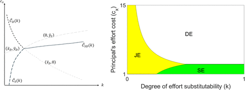
Notes. Sketch of boundaries defined in Proposition 1 (left) and example (right). (Left) Portions of the curves that do not separate operating modes are depicted in light gray; the region with corresponds to JE, to DE, and to SE. (Right) is given by (6), with and .
For any , there exist functions , , and , such that , , and , delineating the FB operating modes as follows:
SE with if and ;
DE with if and ;
JE with if .
When for all , .
As depicted in Figure 2 (left), the FB operating modes can be characterized by three curves: an increasing curve , a decreasing curve , and a curve that lies between the former two; all three curves intersect at the same point. The FB operating mode is SE for any point that lies below both and , DE for any point that lies above both and , and JE otherwise. Given that is increasing and is decreasing, JE tends to dominate when the degree of effort substitutability k is low and when the workers have similar productivity. If JE does not occur, the choice between DE and SE depends on whether lies above or below . In particular, when is symmetric, DE dominates SE if and only if .
The characterization is intuitive: At high levels of degree of effort substitutability k, only the solo operating modes emerge: SE if is low and DE if it is large. This is the situation typically assumed in the PA and task allocation literatures. As k decreases, JE starts to appear, especially when the costs of effort are similar. In fact, one could imagine lowering k so much that efforts would become strategic complements, in which case JE would be the only operating mode, as discussed earlier. This latter situation is typically assumed in the TP literature. This intuitive characterization is consistent with Roels (2014), who considered the particular case of CES functions; Proposition 1 shows that it holds for a much larger class of value functions.
Moreover, the regions in which each operating mode is optimal are coordinate-wise convex. That is, if a particular operating mode is optimal at and at , then so is it at , for any . Also, if it is optimal at and at , then so is it at , for any . As we will see in Section 7, this property breaks down when efforts are chosen in a decentralized way.
5. Equilibrium Operating Modes for a Given Output Share
We next characterize the equilibrium efforts, solving (3) and (4), for any output share . Because the workers’ payoffs are concave and their action sets are convex and bounded, there always exists a pure-strategy Nash equilibrium by the Debreu-Glicksberg-Fan theorem (Fudenberg and Tirole 1991, section 1.3.3). If there exists more than one, the principal selects DE (Lemma B.5).
5.1. Efforts in Each Operating Mode
Similar to the three candidates for local maxima in the FB case (Section 4.1), define the following three candidates for equilibria and specify the conditions under which they are equilibria:
SE:, in which solves ; it is an equilibrium if ;
DE:, in which solves ; it is an equilibrium if ;
JE:, which solves and ; it is an equilibrium if and .
As with the local maxima candidates in the FB case, these potential equilibrium points are uniquely defined and feasible. Moreover, if , ; and if , . Although the second-order optimality conditions do not always hold at the FB local maxima candidates, they always do at these candidate equilibria given that joint concavity of is irrelevant.
5.2. Which Operating Modes Emerge
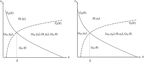
We next characterize which operating modes emerge, for a given . As noted in Section 3.1, the FB efforts solving (1) with inflated costs and also solve (3) and (4). Therefore, the characterization of the equilibrium operating modes for a given follows from the FB solution. This characterization can be done in terms of , as in Proposition 1, or in terms of given that the inflated cost is monotone in . We present the latter version. It is sketched in the left panel of Figure 3 and illustrated numerically in its right panel. Given that is decreasing in , Figure 3 appears almost as a reflection of Figure 2 across the horizontal axis, with a subtle difference when k is large and takes on intermediate values, which corresponds to a situation where , ), and are all equilibria. In this case, the selected equilibrium (preferred by the principal) is DE.
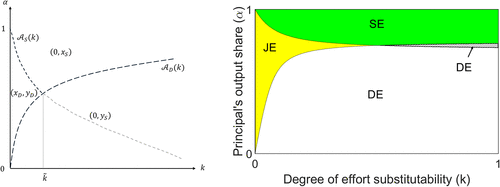
Notes. Sketch of boundaries defined in Lemma 1 (left) and example (right). (Left) Portion of the curve is depicted in light gray whenever it does not distinguish an operating mode. The curves and intersect at . (Right) is given by (6), with , , and . In the striped region in the right panel, all three operating modes are equilibria, out of which the principal selects DE.
For any and , there exist functions and , such that and , delineating the selected equilibrium operating modes as follows:
SE with if and ;
DE with if ;
JE with if .
When increases, both and increase.
As illustrated in Figure 3 (left), the equilibrium operating modes can be mapped in the -space by defining two curves: a decreasing curve and an increasing curve . The equilibrium operating mode is SE for any point that lies above both and , DE for any point that lies below , and JE otherwise. Given that is decreasing and is increasing, JE tends to dominate when the degree of effort substitutability k is low and when is neither too low nor too high. If JE does not occur, the choice between DE and SE depends on whether is above or below .
Denote by the unique solution to . Accordingly, JE may arise in equilibrium if and only if . In particular, when , the equilibrium is DE if , JE if , and SE if . Hence, by varying the agent’s share, the principal can induce different operating modes. Naturally, DE emerges when the agent’s inflated cost is low and the principal’s inflated cost is large, SE emerges when the opposite happens, and JE emerges when the inflated costs take on intermediate values. Notably, DE can only emerge when , in contrast to most PA models, which assume that DE emerges for any .
6. Second-Best Solution
Our second benchmark is the SB solution. We denote by the SB contract that solves (2) subject to (3)–(5). The presence of the fixed fee f effectively decouples the processes of value creation and value capture. Specifically, it is optimal for the principal to set to extract the entire surplus while meeting the agent’s participation constraint. Accordingly, the principal chooses to maximize .
Naturally, if induces either SE or DE in equilibrium, then full efficiency can be achieved in the execution by setting or , respectively, maximizing the principal’s payoff. In the former case, the principal does not form a team; in the latter case, the principal transfers the entire ownership of the project to the agent and captures the entire surplus through the fixed fee. Because the equilibrium efforts are identical to the FB ones under SE and DE, the principal can create and capture all FB value under SE and DE, unlike JE, which is fraught with double moral hazard. As a result, JE emerges (weakly) less often in equilibrium than in the FB.
In the SB, there is too little JE in equilibrium, and too much SE and DE.
With this SB benchmark in mind, we next investigate whether a linear contract also leads to less JE and too much SE and DE, relative to the FB.
7. Linear Contract
We now turn to the equilibrium characterization under a linear contract in the space, keeping constant. Linear contracts are common in intraorganizational settings where financial payments are not allowed. We characterize in Section 7.1 the contract that maximizes (2) subject to (3) and (4) and , denoted as , and compare in Section 7.2 the resulting coproductive dynamics to the FB. Because , we denote the principal’s payoff in (2) as . Throughout our analysis, we ignore the agent’s participation constraint, which, as noted in Section 3.3.5, is not relevant if is sufficiently large.
7.1. Principal’s Optimal Contract
Recall that the FB solution is such that SE does not emerge if and DE does not emerge if (Proposition 1). The next proposition shows that a similar result holds in equilibrium. As discussed at the end of Section 5, is defined as the solution to .
For any , there exists a function such that the equilibrium at is
When , SE if and DE if ;
When , either SE or JE if and either DE or JE if .
Very much like the FB solution, when the degree of effort substitutability is high (), SE emerges as an equilibrium, instead of DE, when the principal’s cost is low. However, is in general not constant, unlike the FB and SB solutions where it sufficed to compare with when is symmetric (Propositions 1 and 2).
Next, consider the case where . In this case, the equilibrium operating mode is DE when , JE when , and SE otherwise (Lemma 1). As noted in Section 3.2, in contrast to the canonical PA model, DE emerges here only when . Otherwise, the principal would have such a large share of output that they could not prevent themselves from contributing to the project execution. Hence, a solution predicated by a canonical PA model may not be achievable when the task has a coproductive nature and the principal cannot commit not to contribute.
This reveals a potential flip side to coproduction: Although it is beneficial to have access to more operating modes from a total surplus (i.e., FB) perspective, it may also constrain the principal’s ability to capture value. In particular, the principal may aspire to capture more value under DE, but to avoid having to contribute to the execution, may find themselves setting . To highlight when this happens, we distinguish two cases under the DE operating mode, depending on whether the principal’s optimization is unconstrained, that is, , which we denote as DEU, or constrained, that is, , which we denote as DEC.
Consequently, the principal may benefit from having a higher cost of effort, so as not to be tempted to contribute. The same behavior may also arise under JE because a less efficient principal will put in less effort, making them rely more on the agent.5 Hence, a higher cost of effort for the principal gives them a higher payoff because it helps them commit not to contribute (Fudenberg and Tirole 1984, Aghion and Tirole 1997).
Considering now the special case where is given by (6), for which , the next proposition shows that, when , the transitions in equilibrium operating modes at as changes are similar to the FB solution in the sense that JE emerges when costs are similar, whereas SE (respectively, DE) dominates when is small (respectively, large). The proposition requires that be sufficiently large that the agent’s participation constraint is nonbinding (Section 3.3.5).
Let be defined as (6) and suppose that (7) holds. For any and k, , the equilibrium at never transitions away from DE as increases and away from SE as decreases.
In contrast, nonmonotone behaviors might emerge in the equilibrium transitions as k changes between the SE and JE operating modes, even in the special case where is given by (6). Specifically, unlike the FB solution, the JE region may not be coordinate-wise convex. That is, if JE is the equilibrium operating mode at for and , it may not be so at , for some . In other words, although JE naturally arises as efforts become less substitutable, JE may also emerge instead of SE as efforts become more substitutable, at least temporarily (Figure 4 (left)).
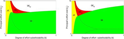
Notes. Here, is given by (6), with and (left) and and (right). The black dashed line represents the boundaries of the FB operating modes (Figure 2). (Left) DE is never FB optimal because . Condition (7) holds when (left) and when (right).
However, this nonmonotone behavior disappears if is sufficiently large, as shown in the next proposition and illustrated in the right panel of Figure 4. The proposition requires that , for some threshold , in addition to requiring that be large enough to ensure the agent’s participation. Note, assuming a sufficiently large , this condition implies that is sufficient for the proposition to hold.
Let be defined as (6) and suppose that (7) holds. For any , there exists a threshold , , such that , the equilibrium at never transitions away from JE as k decreases.
Hence, when the agent’s cost of effort is sufficiently large (and is sufficiently large), JE tends to emerge as the degree of effort substitutability decreases, very much like in FB and SB.
7.2. Comparison with First Best
Unlike the FB/SB comparative statics with respect to and k when the agent’s cost is large (Propositions 1 and 2), here we show that even though there is too much SE in equilibrium, there may not be too much DE or too little JE.
Because there is no agency issue under SE (because ), SE arises in equilibrium whenever it is the FB operating mode. The principal has indeed no incentive to operate differently given that the total value is maximized and the principal can capture all of it. As a result, SE is more prevalent in equilibrium than in the FB.
There is too much SE in equilibrium.
Figure 4 illustrates Proposition 6 and confirms that the region where SE arises in equilibrium (green) is larger than the one in the FB solution (as depicted by the dashed line). We conclude that principals tend to hoard too much so as to retain the full ownership of their project.
Does this hoarding translate into under-delegation? Not necessarily, as demonstrated in the following proposition. Specifically, although there is too little JE when one of the workers has low productivity, there is too little DE otherwise.
Let be defined as (6) and suppose that (7) holds. There exist two thresholds and , such that
When or , there is too little JE in equilibrium;
When and , there is too little DE in equilibrium.
On one hand, there may be too little JE in equilibrium at , like in the SB, and this happens when one of the workers has low productivity (i.e., when either or ). See the right panel of Figure 4 for an illustration.6 This is expected, given that JE is subject to double moral hazard, which is a priori more inefficient than the single moral hazard affecting DE. In this case, principals, whenever they form a team (which happens too infrequently), tend to delegate too much and contribute too little. Paradoxically, over-delegation happens when the agent has low productivity.
On the other hand, there may also be too little DE; this happens when, under the complementary conditions, both workers’ productivities are high (i.e., when and ). See the left panel of Figure 4 for an illustration. In this case, the principal, whenever they form a team (which happens too infrequently), tends to contribute more than they should; that is, there are cases where JE arises in equilibrium, whereas DE would be the FB operating mode. This is motivated by the principal’s desire to capture value as JE provides an opportunity for them to offer a lower share to the agent (i.e., than under DE. This is another form of hoarding, although not as extreme as not forming a team sufficiently often.
How severe is the principal’s project hoarding behavior? To assess this, Figure 5 compares the FB total payoff (top figure), that is, to the equilibrium total payoff (bottom figure), that is, , both depicted with a red solid line. In this numerical study, we used (6) as a functional form for . This comparison is made for two different sets of parameters, corresponding to the left and right panels of the panels. The parameters match those chosen to construct Figure 4.

Note. Here, is given by (6) with , , (left) and , , (right).
For this value function (6), for any ; that is, more value is generated at higher degrees of effort substitutability. Accordingly, both the FB total payoff, depicted in the top panels (red continuous line), and the equilibrium principal’s payoff, depicted in the bottom panels (blue dotted line), are increasing in k as the potential for value creation increases with k.
In addition, Figure 5 reports the corresponding (FB or equilibrium at ) operating modes. As k increases, the equilibrium transitions from JE to SE, to DE, and then back to SE, as shown in the bottom left panel (see also the left panel of Figure 4 when ), or from JE to DE back to SE, as in the bottom right panel (see also the right panel of Figure 4 when ). These transitions are consistent with the equilibrium characterization made in Propositions 3–5. The FB operating mode transitions from JE to DE as k increases (top panels), consistent with Figure 2 and Proposition 1 given that, in both cases (left and right top panels), , so SE is never optimal. Consistent with Propositions 6 and 7, there is too much SE in equilibrium and either too little DE in equilibrium (left panels) or too little JE in equilibrium (right panels).
Unlike the FB total payoff, which continuously increases in k, the equilibrium total payoff exhibits, as k increases, downward jumps whenever the equilibrium operating mode switches to SE and upward jumps whenever it switches away from SE. What explains these jumps is that the agent’s payoff, depicted with a black dashed-dotted line in the bottom panels of Figure 5, discontinuously drops to zero whenever the principal abandons the idea of forming a team and decides instead to work alone (SE), and, conversely, jumps away from zero whenever the principal forms a team and offers incentives to the agent to work on their idea. In contrast, the principal’s payoff, depicted with a blue dotted line in the bottom panels of Figure 5, evolves continuously across the transitions between the different operating modes, irrespective of whether they involve a team. (This discontinuity in the total payoff only arises when the equilibrium operating mode transitions to or from SE because the principal’s optimal share is continuous in k when the equilibrium operating mode switches between DE and JE, resulting in a continuous evolution (as k changes) of both the principal’s and the agent’s payoffs at these transitions.)
Moreover, the loss in total payoff from not forming a team while it would be FB optimal to do so (i.e., when the FB operating modes are either DE or JE, but the equilibrium operating mode is SE) is much more severe than when a team is formed, irrespective of the discrepancy in operating modes (DE or JE) between the equilibrium and the FB and despite the lower execution efforts due to moral hazard. Indeed, a comparison of the top and bottom panels in the figure reveals that, whenever SE is chosen in equilibrium, instead of DE or JE in the FB, the optimality loss is significant. In these regimes, the principal is effectively destroying value through their decision to not form a team.
This highlights a fundamental difference between the moral hazard that affects the effort choice under DE or JE and the lack of control over the principal’s team formation decision. Although the former leads to a loss of value (as shown in the gap between the two red solid curves), the equilibrium total payoff is increasing in k within each operating mode. In contrast, the principal destroys value by switching to SE when k increases, instead of teaming up with the agent. In sum, our analysis suggests that, although most of the PA literature has focused on controlling the agents, it can be even more important to find ways to control principals and curtail their project hoarding behavior.
8. Conclusions
In this paper, we study the genesis of teams in a coproductive PA setting, which arises in numerous OM applications, such as research and innovation, entrepreneurship, service provision, team leadership, franchising, and joint ventures. We consider whether a project initiator—a principal—should share the project value with someone else—an agent—and if so, how. Depending on their respective incentives, one of the following three operating modes may emerge: SE by the principal; DE to the agent, as in the canonical PA model; or JE, as in TP models. Because team production is an “essential,” if not “necessary,” condition for the firm (Alchian and Demsetz 1972, p. 785), explaining when team production (JE) emerges instead of specialization (SE, DE) lies at the core of the theory of the firm. In particular, the development of agentic AI leads to three operating modes: AI only (DE), human only (SE), and human-AI collaboration (JE) (Bastani and Cachon 2025, Fügener et al. 2026).
In a very general setting, we show that JE should arise more when the degree of effort substitutability is lower and the workers’ costs are more similar. Otherwise, the choice between DE and SE is resolved by only considering the respective productivities when the value function is symmetric (Proposition 1). The same coproductive dynamics arise in the second best, attained with an affine contract. However, there is too much SE, too much DE, and too little JE (Proposition 2).
With linear contracts, without financial transfers, under-delegation may also arise, but now due to project hoarding. Specifically, principals partner with agents too little (Proposition 6). Although the coproductive dynamics may exhibit nonmonotonicities that were not present in the FB, JE tends to remain the equilibrium when the degree of effort substitutability is low (Proposition 5). Similarly, SE tends to remain the equilibrium when the principal’s cost is low, as does DE when it is high (Propositions 3 and 4). Although there is too little JE in equilibrium when one of the workers has low productivity, there is too little DE otherwise (Proposition 7). Hence, although project hoarding always takes place, under-delegation occurs when principals are more involved than they should. Relative to the well-documented issue of moral hazard in the PA and TP literatures, hoarding appears to have a more severe impact on value, potentially destroying it despite improvements in the potential value that can be created as a result of a reduction in the degree of effort substitutability (Figure 5).
Our work raises a cautionary tale regarding the value of coproduction. Although coproduction is often perceived to be beneficial because it expands the set of operating modes by potentially involving the principal in production, offering more flexibility to achieve greater efficiency (Proposition 1), it may not benefit principals who may find themselves too constrained in setting incentives for agents under DE. Hence, principals may actually be better off moving away from coproduction and instead exaggerating their costs. Consequently, despite all its praise (Vargo and Lusch 2004), coproduction may not be a panacea in practice.
The proposed approach can be extended in numerous ways. First, we ignored the role of uncertainty, which could potentially lead to information asymmetry and adverse selection (Radner 1993, Aghion and Tirole 1997) and recourse action in a dynamic setting. Second, we considered a single agent, but the model could easily be extended to account for multiple identical agents. Future research could investigate the effect of agent heterogeneity on a project’s operating mode and performance. Third, we only considered one task, but one could generalize the approach to a multitask setting, perhaps with different degrees of effort substitutability, some of which are potentially preassigned to the principal and/or the agent, as in Itoh (2001), Hagiu and Wright (2019), or Bellos and Kavadias (2021). Relatedly, one could extend the model to span over multiple periods and adopt a process perspective, perhaps making the distinction between different phases of execution and characterizing the operating dynamics as the team makes progress or time goes by, in the same vein as Bonatti and Hörner (2011) or Bellos and Kavadias (2021). Fourth, one could investigate the performance of ex post output share allocations, such as bargaining (Bhaskaran and Krishnan 2009) or making shares proportional to effort contributions (Moyer 2016).
Our analysis draws attention to project hoarding in the team formation phase of coproductive dynamics, which may be associated with a more severe loss of efficiency than the moral hazard in the project execution phase (which is the focus of the PA and TP literature). Although our approach is generic in highlighting the salience of this issue across contexts, the identification of mechanisms to prevent principals from engaging in project hoarding would need to rely on more specific models tailored to the particular application context.
Appendix A. Closed-Form Expressions When Is Given by (6) with
A.1. First-Best Solution
When is given by (6), , , and if ,
If and , for any and such that . If and , is not defined. When , is only a saddle point because the determinant of the Hessian matrix (which has negative diagonal elements) is then negative.
A.2. Equilibrium Solution
When is given by (6),
If and , for any and such that . If and , is not defined.
The boundaries delineating the regions where the different operating modes emerge (Lemma 1) are
Because if and only if (iff) , it follows that .
Note. lying above (respectively, below) , (respectively, ). lying above (respectively, below) , (respectively, ).

Note. Π(α) is depicted in red, ΠDE(α) = αV (0, yS(α)) is depicted with short dashes, ΠJE(α) = αV (xD(α), yD(α)) − cxxD(α) is depicted with long dashes, and ΠSE(α) = αV (xS(α), 0) − cxxS(α) is depicted with long dashes-dots.
Appendix B. Proofs of Statements with a Generic Value Function
B.1. First-Best Solution
The proof of Proposition 1 builds on two geometric arguments. The first relies on Figure B.1 to show that (1) has either two local maxima (namely, and ) or a unique one among the three candidates (Lemma B.1).
The second argument, which relies on Figure B.2 (left), leads to the construction of the functions: () below (above) which () is a critical point (Lemma B.2). Accordingly, holding constant, the space can be partitioned into four regions depending on whether the local maxima are only ; only ; only ; or both and (Lemma B.3; Figure B.2 (left)). In the latter case, the maximum of (1) can be identified by comparing the total payoffs obtained at each of these points; the behavior of the delineating boundary can be characterized with the implicit function theorem (IFT).
Among the potential local maxima of (1), namely, , , and , either only one is critical or they all are; in the latter case, is a saddle point.
Let and . By the univalence theorem (Gale and Nikaidô 1965, theorem 7(ii)), and intersect at most once in the positive orthant. Because and efforts are strategic substitutes, is downward-sloping (Figure B.1): lying above ; and lying below . The case of is similar. Finally, is guaranteed to cross the x axis on [0, 1] at because by assumption in Section 3.3.2; crosses the y axis when at .
Consider the conditions that ensure that , , and are critical points. First, is a feasible critical point iff and intersect in the positive orthant. Second, is a critical point iff lies above when it crosses the x axis. Third, is a critical point iff lies above when it crosses the y axis. No two conditions can hold without the third. Moreover, , iff ; hence, is a saddle point. □
If is a local maximum of (1) for some and , it remains so and . Similarly, if is a local maximum for some and , it remains so and .
When is a critical point, at : . The left-hand side is decreasing in k, by Equation (8), and increasing in , as we show next. Applying IFT to shows that is decreasing in . The total derivative of at with respect to , , is thus nonnegative as efforts are strategic substitutes. The proof for is similar. □
For any , functions and , so that and , delineating local maxima of (1): iff ; iff ; and iff .
When is a local maximum, the set of parameter values for which this holds is coordinate-wise convex and expands as k increases and decreases (Lemma B.2). Let denote the increasing region boundary, such that , if is never a local maximum ; and if is always a local maximum . That is, , is a local maximum iff .
Similarly, the parameter set where is a local maximum is coordinate-wise convex and expands as either k or increases. Let denote the boundary of that region, which is decreasing, and using the same extensions to zero and as for . Hence, , is a local maximum iff .
When , neither nor are local maxima. By Weierstrass’s theorem, must be the sole local maximum when .
By Lemma B.1, the number of critical points for maxima is either one or three. Accordingly, cannot be critical when either and , or and . Also, must be critical when and ; however, in that case, is only a saddle point (Lemma B.1). □
Fix . Lemma B.3 characterizes a unique maximum in the following cases: when and ; when and ; and when (Figure B.2). In the remaining case——both and are local maxima, so the global maximizer is iff and otherwise. Applying IFT to (valid as the derivative of the left-hand side with respect to equals ), there exists a function such that iff . Hence, if , (respectively, ) is the global maximum if (respectively, ). Given that the global maximum is when and when , .
When is symmetric, . Hence, iff , that is, iff . Hence, . □
We close this section on the FB by deriving a result that will be useful in our analysis of the linear contract. The result builds on the geometric constructs and introduced in Lemma B.3. Let be the unique solution of . If , namely, the solution to and , can have negative elements, then, when , if and if . Because efforts are strategic substitutes, this implies that if and if . If (respectively, ) can only be nonnegative, then (respectively, ).
Fix . When , is such that if and such that if .
Fix . For any , and maximizes (1) by Proposition 1. Using the geometric constructs of Lemma B.1 (Figure B.1), there exist two downward-sloping curves and in the -space crossing in the positive orthant (at ), and crosses from above. Because shifts downward as increases, whereas is independent of , the crossing point between and shifts to the orthant where and when increases and to the orthant where and when decreases. □
B.2. Equilibrium Operating Modes for a Given Output Share
The proof of Lemma 1 operates in two steps. First, we characterize the equilibrium operating modes of (3) and (4) in the -space, similar to the FB characterization made in Proposition 1 (Lemma B.6; Figure B.2 (right)). The characterizations are similar given that the candidates for equilibrium efforts , , and solve the same first-order conditions as the candidates for local maxima in (1) with inflated costs and . Recall that the FB characterization involves a region with multiple critical points, including (Figure B.2 (right)). Similarly, there is a region with multiple equilibria, including . In this case, is the selected equilibrium (Lemma B.5). Second, we characterize the equilibrium operating modes in the -space because the principal’s cost can be increased by either increasing or decreasing , so a one-to-one mapping exists.
When (3) and (4) have multiple equilibria, the principal always selects DE if it is an equilibrium.
Suppose and are equilibria. Because efforts are strategic substitutes, . As is increasing, . Hence, , that is, .
Suppose and are equilibria. As and is increasing, . Hence, , that is, . □
For any and an increasing function and a decreasing function that delineate the selected equilibrium operating modes: SE with if and ; DE with if ; and JE with if . As increases, both and increase.
The equilibrium conditions for , , and identify the critical points to maximize subject to , which is the FB objective function with inflated costs. The increasing and decreasing functions and define the critical points and unique equilibria (Lemma B.3): when and ; when and ; and when . When , is selected amongst multiple equilibria (Lemma B.5).
We next show the comparative statics with respect to . Suppose for any given , is an equilibrium. Then, at . From ’s equilibrium condition, increases in (IFT). Consider the total derivative of the left-hand side of the inequality with respect to : . It is negative because efforts are strategic substitutes and increases in ; the inequality is thus easier to satisfy for larger . Because is an equilibrium iff , increases in . A symmetric argument holds when is an equilibrium, noting that is an equilibrium iff ; hence, increases in . □
Functions and are monotone in and k, so can be inverted (Lemma B.6). □
We close this section by deriving a result that will be useful in our analysis of the linear contract (Lemmas B.10 and B.11). The result builds on the geometric constructs and introduced in Lemma B.6. Let be the unique solution of . If is such that , namely, the solution to and , can have negative coordinates, then, when , if and if (Lemma B.7). Because of the one-to-one mapping between and , the same result can be expressed in terms of : when , if and if (Lemma B.8). Because efforts are strategic substitutes, this implies that if and if . If is such that (respectively, ) can only be nonnegative, then (respectively, ).
Fix . When , when and when .
The proof is identical to the proof of Lemma B.4. □
Fix . When , (and thus, ) when and (and thus, ) when .
The result follows from Lemma B.7 because and are monotone in and k, so can be inverted. □
B.3. Second-Best Solution
Proposition 2 follows from the fact that the total net value when either SE or DE is the FB operating mode can be achieved in equilibrium.
If : ; if : ; if : . □
B.4. Linear Contract
To characterize the equilibrium operating mode with the optimal contract, rewrite the principal’s payoff in (2), leveraging Lemma 1, as follows:
We define , , and . As we show next, is convex, implying that the maximum is attained at one of the endpoints; hence, . Moreover, if the principal earns strictly positive profit under SE, then .
If such that , then .
The function is convex since by the envelope theorem, is increasing in x, and is increasing in . Therefore, . Because , if for some , then , that is, . □
We next characterize . Let be the solution to . Suppose first that . Then, (Figure 3(b) (right)). DE is the selected equilibrium when , and SE is the selected equilibrium when . In fact, DE is the only equilibrium when , and SE is the only equilibrium when (see Lemma 1 and Figure 3 (right)). In particular, is not positive (and therefore JE is not an equilibrium) when or when , which is why the curve is depicted in light gray in these disconnected regions. When , all three candidate points, namely, , , and , turn out to be equilibria (Figure 3 (right)), but dominates and (Lemma B.5), so DE is the selected equilibrium. is discontinuous (but upper semicontinuous) at . The optimal could lie in (DE) or at one (SE).
Suppose next that . Then, (Figure 3(b) (left)). DE is the only equilibrium when , JE is the only equilibrium when , and SE is the only equilibrium when (see Lemma 1 and Figure 3 (right)). Whenever is not positive (and therefore JE is not an equilibrium), the curve is depicted in light gray. In particular, when and when (Lemma B.7). When , lies above , and it crosses it from above at (Lemma B.10). lies above if and only if ; it thus crosses it from above (Lemma B.11). The optimal could lie in (DEU), at (DEC), in (JE), or at 1 (SE). Even if may lie above when , the principal cannot induce DE because is not an equilibrium when . Specifically, the principal cannot refrain from increasing their effort. Anticipating this, the agent lowers their effort, making the only possible equilibrium.
We first establish that the principal prefers DE over SE iff . By Lemma B.9, . Because , the principal prefers DE over SE iff .
Consider this profit difference: . Recall that is independent of by definition. Applying the envelope theorem, the total derivative of the profit difference between DE and SE can be expressed as . Either or and ; in the latter case, recall that is increasing in by Lemma 1. Hence, the right-hand side is greater than or equal to and the profit gap grows with . Accordingly, larger values of make it easier for DE to dominate SE; that is, there exists a function such that the principal prefers DE over SE iff . □
When , lies above when and crosses from above at (Lemma B.10), and is below iff and thus crosses it from below at (Lemma B.11).
When , and . Hence, at .
When , by Lemma B.8. Therefore, , in which the last inequality holds because is strictly increasing in y. Conversely, when , by Lemma 1. Therefore, . Taking the limit on both sides when , we obtain that at . □
When , iff . Hence, at .
When , by Lemma B.8. Therefore, , in which the first inequality holds because is strictly increasing in x. Conversely, when , by Lemma 1. Therefore, . □
The proofs of Propositions 4 and 5 rely on the requirement that be given by (6) and appear in the Online Appendix.
To compare the equilibrium operating modes with the FB ones, define, similar to (B.2)–(B.4): , , and when and otherwise. (Recall from Section 4.1 that and are always guaranteed to be positive, whereas , defined as the solution to the first-order optimality condition, may not be so.) Accordingly, the FB optimization problem (1) can be reformulated as follows: .
On the one hand, . On the other hand, and . Hence, if , then . □
The proof of Proposition 7 appears in the Online Appendix.
1 Matt Garman, AWS CEO, December 2025, https://stratechery.com/2025/aws-reinvent-agents-for-aws-nova-forge/, accessed in February 18, 2026.
2 See https://ai.ac/, accessed in January 2026.
3 To test the robustness of our findings with respect to this assumption of no commitment, we consider, in Section EC.2 in the Online Appendix, the polar case where the principal can freely commit to an effort level before the agent chooses theirs; the characterization of equilibrium operating modes turns out to be very similar to the case with simultaneous efforts, even though it now becomes possible for the principal to induce DE by committing to exerting zero effort.
4 The univalence theorem (Gale and Nikaidô 1965, theorem 7(ii)) guarantees, when , that there is at most one solution to the following system of equations: and , when . It applies here because the second partial derivatives do not change sign (given that is coordinate-wise concave and efforts are strategic substitutes).
5 For instance, when is given by (6), with , and , the principal’s payoff is increasing in over [8.35, 11.7], when the equilibrium operating mode at happens to be DEC or JE. In contrast, the principal’s payoff is decreasing in when SE is the equilibrium and constant with respect to when DEU is the equilibrium. This behavior disappears when the principal commits to an effort level before the agent because the principal fully internalizes the agent’s response. Applying the envelope theorem to the principal’s payoff shows that the principal’s payoff decreases in under JE in the sequential case.
6 In the left panel, and , so this meets the conditions of the second case in Proposition 7; in the right panel, , so this meets the conditions of the first case in Proposition 7; is defined in the proof of Lemma EC.11 as the smallest value of for which (EC.6) does not have a solution for any k.
References
- (1997) Formal and real authority in organizations. J. Political Econom. 105(1):1–29.Crossref, Google Scholar
- (1972) Production, information costs, and economic organization. Amer. Econom. Rev. 62(5):777–795.Google Scholar
- (2018) Incentive programs for reducing readmissions when patient care is co-produced. Production Oper. Management 27(6):999–1020.Crossref, Google Scholar
- (2000) Information, contracting, and quality costs. Management Sci. 46(6):776–789.Link, Google Scholar
- (2025) The human-AI contracting paradox. Preprint, submitted December 29, http://dx.doi.org/10.2139/ssrn.5962739.Google Scholar
- (2019) When should customers control service delivery? Implications for service design. Production Oper. Management 28(4):890–907.Crossref, Google Scholar
- (2021) Service design for a holistic customer experience: A process framework. Management Sci. 67(3):1718–1736.Link, Google Scholar
- (1998) Venture capital financing, moral hazard, and learning. J. Bank. Finance 22(6–8):703–735.Crossref, Google Scholar
- (2009) Effort, revenue, and cost sharing mechanisms for collaborative new product development. Management Sci. 55(7):1152–1169.Link, Google Scholar
- (1995) Double-sided moral hazard and the nature of share contracts. RAND J. Econom. 26(4):761–781.Crossref, Google Scholar
- (2011) Collaborating. Amer. Econom. Rev. 101(2):632–663.Crossref, Google Scholar
- (2003)
Supply chain coordination with contracts . Graves SC, de Kok AG, eds. Handbooks in Operations Research and Management Science: Supply Chain Management, vol. 11 (Elsevier B.V., North Holland), 227–339.Google Scholar - (2005) Supply chain coordination with revenue-sharing contracts: Strengths and limitations. Management Sci. 51(1):30–44.Link, Google Scholar
- (2025) Implications of team submissions in open innovation contests. IMA J. Management Math. 36(1):1–19.Google Scholar
- (2015) Robustness and linear contracts. Amer. Econom. Rev. 105(2):536–563.Crossref, Google Scholar
- (2003) Financing and advising: Optimal financial contracts with venture capitalists. J. Finance 58(5):2059–2085.Crossref, Google Scholar
- (2021) Revisiting the role of collaboration in creating breakthrough inventions. Manufacturing Service Oper. Management 23(5):1005–1024.Link, Google Scholar
- (1996) Performance verifiability and output sharing in collaborative ventures. Management Sci. 42(1):93–109.Link, Google Scholar
- (2001) Shared-savings contracts for indirect materials in supply chains: Channel profits and environmental impacts. Management Sci. 47(7):881–893.Link, Google Scholar
- (2005) Optimal shared-savings contracts in supply chains: Linear contracts and double moral hazard. Eur. J. Oper. Res. 163(3):653–667.Crossref, Google Scholar
- (2017) Licensing contracts: Control rights, options, and timing. Management Sci. 63(4):1131–1149.Link, Google Scholar
- (2019) Encouraging help across projects. Management Sci. 65(3):1408–1429.Link, Google Scholar
- (2008) Financing the entrepreneurial venture. Management Sci. 54(1):151–166.Link, Google Scholar
- (2025) Optimal skill diversity in teams. Econom. Theory (November 22), https://doi.org/10.1007/s00199-025-01690-0.Crossref, Google Scholar
- (1984) The fat-cat effect, the puppy-dog ploy, and the lean and hungry look. Amer. Econom. Rev. 74(2):361–366.Google Scholar
- (1991) Game Theory (MIT Press, Cambridge, MA).Google Scholar
- (2026) Roles of artificial intelligence in collaboration with humans: Automation, augmentation, and the future of work. Management Sci. 72(1):538–557.Link, Google Scholar
- (1965) The Jacobian matrix and global univalence of mappings. Math. Ann. 159(2):81–93.Crossref, Google Scholar
- (1995) Moral hazard and risk spreading in partnerships. RAND J. Econom. 26(5):591–613.Crossref, Google Scholar
- (2014) Projects and team dynamics. Rev. Econom. Stud. 82(1):187–218.Crossref, Google Scholar
- (2014) Project design with limited commitment and teams. RAND J. Econom. 45(3):598–623.Crossref, Google Scholar
- (2004) Revenue-sharing vs. wholesale-price contracts in assembly systems with random demand. Production Oper. Management 13(1):23–33.Crossref, Google Scholar
- (1986) The costs and benefits of ownership: A theory of vertical and lateral integration. J. Political Econom. 94(4):691–719.Crossref, Google Scholar
- (2019) Controlling vs. enabling. Management Sci. 65(2):577–595.Link, Google Scholar
- (1979) Moral hazard and observability. Bell J. Econom. 10(1):74–91.Crossref, Google Scholar
- (1982) Moral hazard in teams. Bell J. Econom. 13(2):324–340.Crossref, Google Scholar
- (1987) Aggregation and linearity in the provision of intertemporal incentives. Econometrica 55(2):303–328.Crossref, Google Scholar
- (1991) Multitask principal–agent analyses: Incentive contracts, asset ownership, and job design. J. Law Econom. Organ. 7(special issue):24–52.Crossref, Google Scholar
- (1994) The firm as an incentive system. Amer. Econom. Rev. 84(4):972–991.Google Scholar
- (2001) Job design and incentives in hierarchies with team production. Hitotsubashi J. Commerce Management 36(1):1–17.Google Scholar
- (2021) The rise of research teams: Benefits and costs in economics. J. Econom. Perspective 35(2):191–216.Crossref, Google Scholar
- (1993) The stages of team venture formation: A decision-making model. Entrepreneurship Theory Practice 17(2):17–27.Crossref, Google Scholar
- (2020) The k-index is introduced to replace the h-index to evaluate better the scientific excellence of individuals. Heliyon 6(7):e04415.Crossref, Google Scholar
- (1995) Service markets and competition. J. Oper. Management 12(3–4):397–411.Crossref, Google Scholar
- (2009) The effects of problem structure and team diversity on brainstorming effectiveness. Management Sci. 55(12):1899–1913.Link, Google Scholar
- (1976) Decisions with Multiple Objectives: Preferences and Value Tradeoffs (Wiley, New York).Google Scholar
- (2013) Collaborative cost reduction and component procurement under information asymmetry. Management Sci. 59(1):189–206.Link, Google Scholar
- (1998) Linear contracts and the double moral-hazard. J. Econom. Theory 82(2):342–378.Crossref, Google Scholar
- (2017) Self-managing organizations: Exploring the limits of less-hierarchical organizing. Res. Organ. Behav. 37:35–58.Crossref, Google Scholar
- (2009) Optimal ownership in joint ventures with contributions of asymmetric partners. J. Econom. 97:141–163.Google Scholar
- (2016) Slicing Pie Handbook: Perfect Equity Splits for Startups (Lake Shark Ventures, Lake Forest, IL).Google Scholar
- (2002) Sharing rules in teams. J. Econom. Theory 107(2):407–420.Crossref, Google Scholar
- (1995) A theory of responsibility in organizations. J. Labor Econom. 13(3):387–400.Crossref, Google Scholar
- (2002) The tenuous trade-off between risk and incentives. J. Political Econom. 110(5):1071–1102.Crossref, Google Scholar
- (1993) The organization of decentralized information processing. Econometrica 61(5):1109–1146.Crossref, Google Scholar
- (2017) Collaborative work dynamics in projects with co‐production. Production Oper. Management 26(4):686–703.Crossref, Google Scholar
- (2018) Team leadership and performance: Combining the roles of direction and contribution. Management Sci. 64(11):5234–5249.Link, Google Scholar
- (2014) Optimal design of coproductive services: Interaction and work allocation. Manufacturing Service Oper. Management 16(4):578–594.Link, Google Scholar
- (2010) Contracting for collaborative services. Management Sci. 56(5):849–863.Link, Google Scholar
- (2007) R&D alliances and firm performance: The impact of technological diversity and alliance organization on innovation. Acad. Management J. 50(2):364–386.Crossref, Google Scholar
- (2007) Incentives that induce task-related effort, helping, and knowledge sharing in workgroups. Management Sci. 53(10):1533–1550.Link, Google Scholar
- (2010) Lone inventors as sources of breakthroughs: Myth or reality? Management Sci. 56(1):41–56.Link, Google Scholar
- (1999) Coordinating investment, production, and subcontracting. Management Sci. 45(7):954–971.Link, Google Scholar
- (2004) Evolving to a new dominant logic for marketing. J. Marketing 68(1):1–17.Crossref, Google Scholar
- (2004) Staged financing in venture capital: Moral hazard and risks. J. Corporate Finance 10(1):131–155.Crossref, Google Scholar
- (2004) Incentives and discrimination. Amer. Econom. Rev. 94(3):764–773.Crossref, Google Scholar
- (2007) The increasing dominance of teams in production of knowledge. Science (1979) 316(5827):1036–1039.Google Scholar
- (2012) The impact of royalty contract revision in a multistage strategic R&D alliance. Management Sci. 58(12):2251–2271.Link, Google Scholar
- (2016) The time–Money trade-off for entrepreneurs: When to hire the first employee? Manufacturing Service Oper. Management 18(4):559–569.Link, Google Scholar