
Information Retrieval Under Network Uncertainty: Robust Internet Ranking
Abstract
Internet ranking algorithms play a crucial role in information technologies and numerical analysis due to their efficiency in high dimensions and wide range of possible applications, including scientometrics and systemic risk in finance (SinkRank, DebtRank, etc.). The traditional approach to internet ranking goes back to the seminal work of Sergey Brin and Larry Page, who developed the initial method PageRank (PR) in order to rank websites in search engine results. Recent works have studied robust reformulations of the PageRank model for the case when links in the network structure may vary; that is, some links may appear or disappear influencing the transportation matrix defined by the network structure. We make a further step forward, allowing the network to vary not only in links, but also in the number of nodes. We focus on growing network structures and propose a new robust formulation of the PageRank problem for uncertain networks with fixed growth rate. Defining the robust PageRank in terms of a nonconvex optimization problem, we bound our formulation from above by a convex but nonsmooth optimization problem. Driven by the approximation quality, we analyze the resulting optimality gap theoretically and demonstrate cases for its reduction. In the numerical part of the article, we propose some techniques which allow us to obtain the solution efficiently for middle-size networks avoiding all nonsmooth points. Furthermore, we propose a coordinate-wise descent method with near-optimal step size and address high-dimensional cases using multinomial transition probabilities. We analyze the impact of the network growth on ranking and numerically assess the approximation quality using real-world data sets on movie repositories and on journals on computational complexity.
Funding: This work was supported by the Austrian Science Fund [Grant J3674-N26].
Supplemental Material: The online appendices are available at https://doi.org/10.1287/opre.2022.2298.
1. Introduction and Literature Review
PageRank (PR) is an automated information retrieval algorithm that was designed by Sergey Brin and Larry Page (Brin and Page 1998, Page et al. 1998) during the rise of the World Wide Web in order to improve the quality of search engines existing at that time. The algorithm relies not only on keyword matching but also on the additional structure present in the hypertext, resulting, therefore, in a higher-quality ranking.
Nowadays, different adaptations of the PageRank algorithm are successfully applied in a huge variety of areas (Agarwal and Venkatesh 2002, Aladwani and Palvia 2002, Pant and Sheng 2015, Lappas et al. 2016), starting with straightforward applications such as scientometrics (Liao et al. 2019, Xu et al. 2011), where ranking algorithms are used for measuring the importance of scientific literature, and social media, to seemingly unrelated fields such as financial risk management, where ranking is employed for the measurement of systemic risk in the banking sector (Sadoghi 2015, Chen et al. 2016, Capponi et al. 2020). In our article, we present the results in the context of web ranking; however, our findings can be easily applied in a wide variety of other areas.
The initial idea of the PageRank algorithm (Brin and Page 1998, Page et al. 1998) is based on the interchange of ranks between web pages in line with probability theory rules: a web page gives a part of its rank (or score) only to those web pages that it cites, that is, to which it refers with direct links. The amount of the transferred score is proportional to the probability for a random user to click on the link. In the initial PageRank formulation (Page et al. 1998, Bryan and Leise 2006, Langville and Meyer 2006, Franceschet 2011), this probability is assumed to be an inverse of the total number of links outgoing from a page. This implies equally probable transitions for a random user from some page to the pages cited on it. Similarly, transitions to referred pages are assumed to be uniform for huge-dimensional web ranking in practice. In general, though, this might not be true, as the user is more likely to move to the page with a higher rank than to the page with a lower rank. Therefore, for a better ranking quality, the transition probabilities should be assumed to be rank-dependent. One step forward is made in scientometrics, where the transition probabilities between journals are not uniform but are proportional to the number of cited articles belonging to the same journal (Timonina 2009, Xu et al. 2011). In our article, we make a further step forward, constructing a robust reformulation of the PageRank problem allowing transition probabilities to vary in a given ambiguity set.
The PageRank problem can be formulated as the problem of finding the principal eigenvector of a nonnegative transition matrix, where each column consists of transition probabilities from the corresponding page to all other pages. The principal eigenvector is not necessarily unique for nonnegative stochastic matrices (Horn and Johnson 1990). To impose uniqueness, the original PageRank problem is replaced with finding the principal eigenvector of a modified matrix with only positive components in the works (Brin and Page 1998, Page et al. 1998, Franceschet 2011). This matrix, known as the Google matrix, is used in practice and assumes a possibility of random transitions between pages. In the pioneering paper of Brin and Page (1998, section 2.1.2), the following intuitive justification is given to the matrix: “We assume there is a ‘random surfer’ who is given a web page at random and keeps clicking on links, never ‘hitting back’ but eventually gets bored and starts on another random page. The probability that the random surfer visits a page is its PageRank. And, the damping factor is the probability at each page the ‘random surfer’ will get bored and request another random page.” In the work of Polyak and Timonina (2011), it is shown that the principal eigenvector may be significantly influenced by this difference in matrices, and, importantly, for specific network structures, it may happen that the eigenvector of the Google matrix stops distinguishing between high-ranked pages that build the core of search engine results: if a large amount of high-ranked pages obtains the same score, then the ranking becomes ineffective, making the difference between “high-ranked” and “low-ranked” pages to be almost binary. In our article, we show that the Google matrix provides an approximate solution for the robust case with uniform probabilities. However, it accounts for neither rank-dependent transition probabilities nor a rapid network growth.
Generally, the approach with the modified matrix works well in the presence of a small number of high-ranked pages, which was true when the initial algorithm (Brin and Page 1998) was developed but which currently needs reconsideration as the amount of information on the web continues to grow and the number of experienced users in web research is increasing. In the work of Polyak and Timonina (2011), the authors propose an l1-regularization method that avoids low-ranked pages. This optimization problem can be solved simply via the coordinate-wise descent method analogous to the Gauss-Seidel algorithm for solving linear equations (Polyak 1987, Tibshirani 1996, Bryan and Leise 2006, Langville and Meyer 2006, Polyak and Timonina 2011), enhancing efficiency of numerical ranking and improving accuracy by differentiating between high-importance pages. However, this optimization problem has a drawback: it is not robust to variations in the internet structure, while the World Wide Web is, clearly, changing over time; the amount of information on the web is growing, new pages appear, and some websites (old or spam sites) disappear (Zhu et al. 2014, Lappas et al. 2016, De los Santos and Koulayev 2017, Negahban et al. 2017). This is particularly important due to the fact that PageRank computation takes such a significant amount of time (Google reevaluation of PageRank takes weeks; Nazin and Polyak 2009) and around 1%–3% of new web pages open during this time with new links influencing the transportation matrix.
In the work of Juditsky and Polyak (2012), the robust PageRank model is proposed for networks, whose links may vary, influencing the transition matrix of a fixed dimension. Thus, by solving this problem, one obtains robust ranking for the case when the connections change. As for the internet, (i) the number of pages grows, and (ii) one does not explicitly know how the structure changes. In this article, we study networks which vary not only in links but also in the number of nodes, and we therefore consider growing structures. This is one of the main contributions of our work: allowing for the network growth.
Considering the growth rate to be fixed for the network, we formulate the robust PageRank in terms of a nonconvex optimization problem and bound this formulation from above by a strictly convex but nonsmooth optimization problem. Given some conditions on the parameters suggesting high uncertainty in new pages, the resulting problem appears to be independent of the growth rate and, thus, is also robust to its variations. In middle- to large-dimensional cases, convex nonsmooth optimization problems can be solved numerically using available optimization techniques, including interior-point methods, mirror-descent algorithms (Nemirovski and Yudin 1983, Lan et al. 2012) and randomized techniques (Nazin and Polyak 2009, Ishii and Tempo 2010, Ishii et al. 2005). In huge-dimensional cases, one can employ randomized subgradient algorithms, which are specifically designed for sparse matrices by Nesterov (2014), or first-order extragradient methods, such as Mirror-Prox and dual interpolation algorithms (Nemirovski 2004, Nesterov 2007, Juditsky and Nemirovski 2012). Moreover, one can use less accurate but extremely fast numerical methods proposed by Juditsky and Polyak (2012), Lei (2014), and Polyak and Timonina (2011). In our article, we propose some techniques that allow us to smoothen the optimization problem. We propose a projected subgradient algorithm, avoiding all nonsmooth points, and, furthermore, we develop a coordinate-wise descent method with a near-optimal step size. We also address high-dimensional algorithms in our article.
In Section 2, we propose an l2-norm robust reformulation of the PageRank model with a growing network. Further, we state a separability lemma that plays a crucial role for the robustness: one can conclude under which conditions on the uncertainty the estimated ranking is robust to the network growth. In Section 3, we assess the approximation quality and demonstrate cases for the optimality gap reduction, including the case with zero optimality gap. In Section 4, we propose a coordinate-wise descent method with near-optimal step size. In Sections 5–7, we analyze the convergence and assess the impact of the network growth on ranking using real-world data sets on online movie repositories and on journals on computational complexity.
2. Mathematical Model
Let N be the total number of pages in the internet. The rank of some page , denoted by xi, is the probability for a random user to be on this page. Let be the set of all web pages that refer to page i. The probability that a random user sitting on a page clicks on the link to page i is equal to Pij. The interchange of ranks between pages is formulated in line with probability theory rules as , where the probability Pij is assumed to be an inverse of the total number of links outgoing from page j denoted by nj; that is, .
Next, consider a column-stochastic nonnegative transportation (or transition) matrix , which satisfies , and by definition. The well-known Perron-Frobenius theorem (Horn and Johnson 1990) states that there exists a dominant (or principal) eigenvector , where is the standard simplex on . In general, matrix P is huge-dimensional and very sparse, as the number of links outgoing from every node is much smaller than the total number of nodes in the network: the average number of links outgoing from a web page in the internet is equal to 20 for the whole web (Juditsky and Polyak 2012), while the total number of pages in the internet is approximately 109. The dominant vector describes the stationary distribution on the network structure: each element of the vector denotes the rank of the corresponding node. Components of can also be interpreted as proportions of time that an average user spends on a particular website.
The dominant vector is not robust and may be highly vulnerable to small changes in matrix P, which happen both due to the changes in links and in the number of nodes in the World Wide Web. According to the Web Server Survey (https://news.netcraft.com/archives/category/web-server-survey/), the number of domains being registered per minute corresponds to the 1%– 3% average growth rate of the internet per month. That is why in this article we consider the following changes of matrix P:
We say that matrices P and Q are nonnegative if ξ, ζ, ψ, and χ satisfy the following properties:
In addition, the following properties must hold for column-stochastic matrices Q and P, with a right dominant eigenvector corresponding to the eigenvalue 1:
Similar to the work of Juditsky and Polyak (2012), the function , where is some norm, can be seen as a measure of “goodness” of a vector x as a common dominant eigenvector of the family Ξ, where Ξ stands for the set of perturbed stochastic matrices of the form (1) under Conditions (2) and (3).
Further, let us denote by a feasible point that is a candidate for the common dominant eigenvector of the family Ξ. Let be of the size , and let be of the size . Hence, x is of the size . Note that the vector x must belong to the standard simplex , which means , and (i.e., ).
We say that the vector is a robust solution of the eigenvector problem on Ξ if
The reasonable choice of the uncertainty set Ξ would impose some bounds on the column-wise norms of matrices ξ, ζ, ψ, and χ, meaning that the perturbation in links of the current and future states of the network would be bounded; that is, , and , where denotes the jth column of a matrix. Moreover, the total uncertainty budget for matrices ξ, ζ, ψ, and χ could be fixed (Juditsky and Polyak 2012): this would imply constraints on the overall possible perturbations of the transportation matrix P.
By solving the optimization Problem (4), one would make the rank vector robust to link or node perturbations influencing the transportation matrix P. Currently, the Google scores vector is being updated periodically without accounting for the 1%–3% average monthly growth rate (e.g., Nazin and Polyak 2009 and Internet Live Stats since 2014). By solving the optimization problem of the type (4), one could decrease the number of updates of the score vector and, therefore, reduce the underlying personnel and machinery costs. Furthermore, the resulting ranking would be useful for cutting-edge applications in operations research, operations management, and marketing (Palmer 2002, Dhar et al. 2014, Pant and Sheng 2015, Lappas et al. 2016, De los Santos and Koulayev 2017, Negahban et al. 2017) by providing robust evaluation of the page quality.
We say that the vector is the l2-robust solution of the eigenvector problem on the set of perturbed matrices if
The optimization Problem (5) accounts for uncertainties in links between current and future pages: these uncertainties are incorporated via matrices ξ, ψ, ζ, and χ, whose worst-case realizations lead to the robust PageRank. The optimization problem differs from the robust formulation proposed by Juditsky and Polyak (2012), who studied uncertainties implied by the matrix , describing variations in links of existing pages only. This formulation implies a lower bound on our model.
(Lower Bound). Given , the fixed-size network model imposes a lower bound on the optimization Problem (5) in the following sense:
See Online Appendix A.1 for the proof. Note that we do not require ψ = 0, and, thus, we allow columns of to sum up to values less than or equal to 1 in the left-hand side of the inequality.
Importantly, the network described by Juditsky and Polyak (2012) imposes column-wise conditions but not the nonnegativity constraints . In line with Online Appendix A.1, we can relax these constraints in both sides of Inequality (6). Now, denoting by s the total importance of current N pages, that is, with , we obtain
As the optimization Problem (5) is not convex-concave, the function cannot be computed efficiently. For the computable robust dominant eigenvector of the family of perturbed matrices , we formulate the following theorem, denoting and .
(Upper Bound). The following upper bound holds:
See Online Appendix A.2 for the complete proof. As a consequence, the optimal value of the nonconvex optimization Problem (5) can be bounded from above as
The parameter describes the total uncertainty in links of current N pages, while the parameter describes the uncertainty in links of new M pages. Importantly, both parameters can be chosen independently from the growth M, which makes the resulting vector robust to variations in the number of new nodes. We refer to the vector as the (computable) robust dominant eigenvector of the corresponding family of perturbed matrices if .
In general, this problem is not strictly convex, as the objective function reduces to a constant plus a term proportional to the l1-norm for a fixed x and λ. Nevertheless, functions and are equal to strictly convex l2-norms for large-enough uncertainty parameters and , respectively. When not equal, the objective function can be bounded from above by , which is strictly convex as the sum of a strictly convex and a convex function and, thus, has a unique minimum.
Note that the formulation in (8) coincides with the upper bound proposed by Juditsky and Polyak (2012) if M = 0 (i.e., if there is no growth in the network). In general, for M > 0, the robust reformulation in (8) differs from the l2-bound imposed by the fixed-size network. The exception is the trivial case with ψ = 0 and M > 0, that is, the transition matrix with no links from old to new web pages. This case implies that Q is reducible, meaning that a random user who starts from some new page (among ) and keeps clicking on links eventually results on one of pages as and is not able to return to the starting page by clicking on links as ψ = 0. In this setup, the difference between the fixed-size and the growing network models is fully imposed by the links from new pages, and the ranks are a priori lower than . Furthermore, as one cannot say which of pages have higher ranks and which have lower ones before the internet structure is updated, the ranks could be assumed to be zero without loss of generality, and the problem could be solved numerically using algorithms proposed by Juditsky and Polyak (2012).
In this article, we focus on parameters , and we test the robust setup with in Section 8, where we analyze the influence of the uncertainty budget on ranking of current pages. Clearly, positive uncertainty budgets provide a necessary but not sufficient condition for Q to be irreducible, and, thus, the uncertainty set still includes reducible, as well as periodic transition matrices, for which the eigenvector corresponding to the maximal eigenvalue is not unique. Importantly, as we conclude from Theorem 2, the worst-case realization of Q leads to a formulation that can be bounded from above by a convex optimization problem regardless of possible reducibility or periodicity of Q. Furthermore, it can be bounded by a strictly convex function that has a unique minimum.
Lastly, recall that and due to column-stochasticity of matrix Q. This leads to the requirement , as the optimization Problem (5) would be infeasible otherwise. Also, matrix needs to be nonnegative with none of its columns summing up to values larger than 1. At maximum, and , which happens when matrix ξ nullifies all elements of P redistributing the values among other rows. At minimum, , because P is column-stochastic by itself.
2.1. Robustness and Ambiguity Set
The optimal solution of the optimization Problem (8) is robust to variations in links and to the network growth. Excluding the point from the feasible region in Problem (8), one would logically imply that the uncertainty about current pages is not larger than the uncertainty about future (not yet existent) pages. Instead of cutting this point directly out of the feasible region, we find the exact cases when it may become the optimal solution.
Let and be solutions of the optimization Problems (9) and (10):
See Online Appendix A.3 for the complete proof and note that , as the solution of the minimization Problem (10) is being searched for on the simplex ΣM. Nevertheless, is optimal in Problem (8) under point 1 of Lemma 1. From this follows that the robust setup assigns zero ranks to new nodes before they appear (if is unknown) and ranks currently existing pages only.
According to Lemma 1, the optimization Problem (8) is separable in and : Problem (9) is a convex nonsmooth optimization problem, which we can only solve numerically, whereas Problem (10) is solvable theoretically. Due to this property, we are able to state conditions on , and implying the robustness of an estimated vector of ranks and guaranteeing that the point is never optimal, thus bounding the ambiguity set. To avoid the optimal solution , one needs to make point 2 of Lemma 1 infeasible. In Statement 1, we explicitly solve Problem (10), and we state conditions on parameters , and , which imply the feasibility of points 1 and 3 of Lemma 1.
Let s be the total importance ofcurrent N pages; that is, . Consider the reformulation (8) and change the variables as . In this case, and the following holds:
See Online Appendix A.4 for the proof.
Thus, points 1 or 3 of Lemma 1 are satisfied if
For any , the minimal value of Problem (9) is smaller than ϵ1. This is due to the simplex constraints on and the Perron-Frobenius theorem, which implies that there is such that . Due to the same reasons, the minimal value of the objective function in (9) is smaller than .
Now, if , then the minimal value of Problem (9) is clearly smaller than 1. In this case, the Conditions (12) are sufficiently satisfied for . This implies that, as the number M of new pages increases, the uncertainty about future pages should grow faster than to guarantee that the solution of Problem (9) is robust to variations in links and to the growth in the number of nodes. For M = 1, this is always satisfied. For higher dimensions (i.e., M > 1), we test this condition by computing Google vectors and the corresponding objective values in (9) using subnetworks of a real-world Movies data set with 4,754 nodes (see Section 5).
Next, for a given network of the size N, we denote the objective value of (9) evaluated at the Google vector xG by : note that the Google vector is not necessarily the minimizer of (9); that is, and . In line with the first inequality in (12), the following must hold true for the vector xG robust to variations in network size and structure:
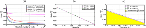
To check the robustness of the Google vector xG for different M, we model the growth of the Movies network. For this, we take a random sequence of increasing submatrices of its adjacency matrix. We start with low values of N and proceed to the actual size of the network (i.e., n = 4,754). We set a 3% growth rate (i.e., nodes) in Figure 1(a) and a 15% growth rate (i.e., nodes) in Figure 1(b). By computing the Google vector for each of the resulting networks, we verify (13) by plotting the function with respect to the number of new pages M, where the value of depends on the network size N. By this, the green area in Figure 1 identifies the values of the uncertainty parameter satisfying (13).
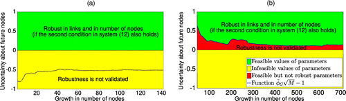
Note. (a) 3% growth rate; (b) 15% growth rate.
If the function takes only negative values as in Figure 1(a), then the robustness criterion in (13) is validated for all feasible values of the uncertainty parameter, that is, for . Conversely, the robustness is not validated for the area below the line (red area for feasible parameters in Figure 1(b)). Overall, the considered sequence of Google vectors satisfies the robustness criterion in (13) at the 3% growth rate of the Movies data set, being, however, not robust at the 15% growth rate for some feasible uncertainty parameters.
Further, note that the applicable growth rate obviously depends on the context of the application. In the web ranking context, if robustness is not validated at higher growth rates but is validated at lower rates, as in Figure 1, then search engines can aim to perform more frequent updates of their rankings using the Google approach in order to match the vector with the growth rate (e.g., five times more frequent updates for the case as in Figure 1). Nevertheless, this is not always possible due to the limitations in computing power, as well as high growth rates, and, more importantly, due to the influence of the chosen method on the position of currently existing pages. In particular, the Google vector may imply a very weak bound on the optimal value of Problem (9) and stop distinguishing between ranks of high-importance pages, as shown by Polyak and Timonina (2011). Further benefits of our approach are demonstrated numerically in Sections 6 and 7 after we describe the solution method in Section 4.
Before we proceed with numerical insights, we theoretically analyze the optimality gap between the optimization Problem (5) and its upper bound implied by Theorem 2 in Section 3.
3. Approximation Quality
Several corollaries of Theorems 1 and 2 provide information on the quality of approximation of the non-convex-concave Problem (5). The quality can be measured both via the distance between optimal values and, importantly, via the difference in optimal solutions, that is, in ranking vectors.
Denoting by Δ the optimality gap between Problem (5) and its approximation (8), we, first of all, state a straightforward bound directly implied by the optimal value of Problem (8) due to the nonnegativity of objective functions. Note that the optimal value is, in turn, bounded from above by and . This is due to simplex constraints on the ranking vector. Furthermore, it is bounded from above by the value , where is the dominant eigenvector of the matrix P. Additionally, . In general, all of these gaps allow us to measure the approximation quality roughly without solving any additional optimization problems.
Next, the optimality gap can be bounded tighter for problems with larger uncertainty about new pages in case the fraction of ranks devoted to old pages is known. This fraction is denoted by and can be estimated from data similar to the parameter M: as soon as we know how many pages appear on average during the month, we can estimate the fraction of ranks that they achieve on average. Also, this fraction can be evaluated using the approach described in Section 4.2. Given s, the optimality gap can be represented as the difference in two optimization problems (see Corollary 1).
Let and . The optimality gap between the initial Problem (5) under constraint and its convex approximation (8) under the same constraint can be bounded by as , where is
See Online Appendix A.5 for the proof. Importantly, the same bound v(s) holds for the optimality gap Δ between Problems (5) and (8) if s underestimates the true importance of current pages optimal in Problem (5); that is, . Also, the bound in (A18) in Online Appendix A.5 holds .
Note that the proposed bound v(s) can be interpreted as the difference between two ranking approaches. In the first one, corresponding to the upper bound , we address both structural and dimensionality changes of the network under the condition that the value of s is known. Conversely, the lower bound taken with c = 1 generalizes the problem described by Juditsky and Polyak (2012) to the case with . Therefore, it describes the network with changes in its structure and with a known fraction of ranks corresponding to new appearing pages. Given this, the optimality gap is equal to if s = 1 and measures the difference between robustness with and without changes in the network size. Also, if we relax the constraint on s in the lower bound , then its value will be equal to zero given the feasible solution . If we further relax the constraint on s in the upper bound, then the optimality gap will reduce to given point 1 in Lemma 1, that is, to the trivial optimality gap between Problems (5) and (8). Additionally, selecting ψ = 0 and given the feasible matrix ξ, we obtain due to the fact that the dominant eigenvector exists for any column-stochastic matrix . Thus, the optimality gap decomposes to the trivial bound for s = 1, ψ = 0, and a given . Further, the optimality gap can be written as
We test the performance of the bound in (15) numerically in Section 8. For this, given samples for matrices ξ and ψ, one could try to solve the nonsmooth convex optimization Problem (14) via subgradient methods. Nevertheless, as the solution would be an approximation providing an upper bound on Problem (14), this would likely result in an underestimation of the gap. As a solution to this numerical issue, we state Propositions 1 and 2, which have closed-form solutions.
Let c = 1. The optimal value of Problem (14) satisfies , where the lower bound has a closed-form solution such that and is invertible. The solution is with .
By setting c = 1 but keeping in the bound in (14), we derive the statement of Proposition 1, where we relax the constraint . The optimal solution is a special case of the well-known least-squares problem under linear constraints (e.g., chapter 16.2 in Boyd and Vandenberghe 2018). Note that the optimal value is not necessarily zero, as is not column-stochastic on , having columns that sum up to values less than or equal to 1 due to nonnegativity of ψ.
Let . The optimal value of Problem (14) satisfies , where the lower bound has a closed-form solution such that and is invertible. The solution has the closed form .
This statement follows from the nonnegativity of the objective function in (14) as . We also relax the constraint and use the optimal solution of the constrained least-squares problem (chapter 16.2 in Boyd and Vandenberghe 2018) representing the objective function as .
In both propositions, we require invertibility of the matrix . Note that the matrix is not invertible, as it is rank-deficient, having columns summing up to zeros. Nevertheless, as invertible matrices are dense in a set of N × N matrices for any norm, one can always find an invertible for nonzero uncertainty parameters and . For this, one requires . Otherwise, the matrix would be column-stochastic by itself, thus, implying the rank deficiency of .
Next, given the invertibility of , the matrix is invertible. This is due to the fact that , where . Matrix A has rank N, as is invertible. This implies that matrix ATA is symmetric and positive definite.
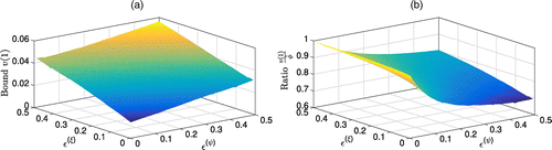
Using Propositions 1 and 2 to compute the lower bounds, we compare the value of v(s) imposed by Corollary 1 with the trivial bound . Thus, we derive the conditions on the total importance of old pages leading to the optimality gaps lower than . Figure 2 demonstrates these conditions for different growth rates. For the analysis, we use the Computational Complexity data set with n = 789 nodes described in Section 5.1. We observe that Proposition 1 results in a broader range of the importance parameter s, providing optimality gaps lower than given large growth rates M. Nevertheless, a small number of new pages M with high uncertainty and lower values of s suggest using Proposition 2.
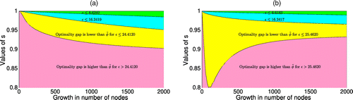
Note. (a) Proposition 1; (b) Proposition 2.
The improvement is achieved in approximately 10% of cases (i.e., s > 0.9) for large M and ϵ in Figure 2(a), whereas this percentage increases as we increase the uncertainty parameters. Similarly, the smallest value of s allowing the reduction of the gap in approximately 20% of cases (i.e., s > 0.8), is obtained at an approximately 12% growth rate in Figure 2(b).
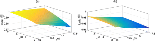
For s = 1, Figure 3 demonstrates the reduction in the ratio and, thus, the improvement of the bound v(1), which is dependent on the values of the uncertainty parameters and . In Figure 3, (a) and (b), we observe that the optimality gap bound implied by Proposition 1 (respectively, Proposition 2) decreases by approximately 2% (respectively, 4%) in case of a 15% network growth given low values of and high values of . Indeed, the objective value of Problem (20), which we employ for the numerical solution (see the upper bound in (19)), increases in and and is symmetrical for and . However, due to the nonlinear dependency of the lower bound on the values of ξ and ψ, the percent reduction of the optimality gap is asymmetrical in the perturbation parameters and . This result is analogous to the one presented in Figure 18 in Section 8.
Note. (a) Proposition 1 15% growth; (b) Proposition 2 15% growth.
Further, Corollary 2 provides an implicit bound for the solution vector of the initial Problem (5) given the optimal value and the solution of the upper bound in (8). Clearly, besides the statement of the Corollary 2, simplex constraints hold for the solution , implying that .
Given and , let be the optimal solution of the reformulation (8), and let be its optimal value. The following implicit inequality holds for the true solution vector :
See Online Appendix A.6 for the proof. One can also state inequalities and , which hold true for all ξ and χ in the uncertainty set. The first inequality follows directly from Theorems 1 and 2. The second one is shown in Online Appendix A.6. Additionally, if the uncertainty set is large enough (i.e., if ), then one can deduce the bound , which combines components corresponding to old and new pages in one statement.
As Inequality (16) depends solely on the uncertainty matrix ξ, it provides some possibilities for numerical tests demonstrated in Section 8. Conversely, the bounds involving ranks of new pages require a generation of random matrices χ and become more complex to validate as the number M of new pages grows. Note also that the worst-case perturbations in the left-hand side of the proposed inequalities cannot be computed explicitly because of the functional form and constraints of the problems.
Lastly, we demonstrate a degenerate case that implies zero optimality gap between a modified Problem (5) and its approximation. For this, we consider the set of constraints and the following optimization problem,
Given , the following bounds hold for the optimization Problem (17):
Furthermore, if and , then the optimality gap , where
See Online Appendix A.7 for the proof and a small-dimensional example.
In Section 8, we numerically analyze Corollaries 1 and 2 for real-world data sets, considering pessimistic and optimistic scenarios with a boost growth in the number of new pages M. This allows us to assess theoretical and empirical values of optimality gaps, as well as to observe possible true solution patterns.
In Section 4, we propose solution methods for middle- and high-dimensional problems. For this, recall that Problem (8) can be subdivided into two separate smaller-size optimization problems in line with Lemma 1¸whereas Problem (10) can be solved explicitly. Thus, we focus on the convex but nonsmooth optimization Problem (9) of the type described in the works of Ben-Tal and Nemirovski (1998), Boyd and Vandenberghe (2004), and Juditsky and Polyak (2012) with :
Similar to Juditsky and Polyak (2012), we develop numerical algorithms for the right-hand side in (19), as it bounds the initial Problem (5) and is strictly convex and provides zero optimality gap with (17) under the conditions of Corollary 3.
4. Solution Method
In middle- to large-dimensional cases (i.e., ), the convex nonsmooth optimization Problem (19) can be solved numerically using available optimization techniques, including interior-point methods, mirror-descent algorithms (Nemirovski and Yudin 1983, Lan et al. 2012) and randomized techniques (Ishii et al. 2005, Nazin and Polyak 2009, Ishii and Tempo 2010). In huge-dimensional cases (i.e., ), one can employ randomized subgradient algorithms, which are specifically designed for sparse matrices by Nesterov (2014), or first-order extragradient methods, such as mirror-prox and dual interpolation algorithms (Nemirovski 2004, Nesterov 2007, Juditsky and Nemirovski 2012). Moreover, one can use less accurate but extremely fast numerical methods proposed by Juditsky and Polyak (2012), Lei (2014), and Polyak and Timonina (2011). In this section, we propose techniques that allow us to smoothen the optimization Problem (19), and we develop numerical algorithms for the solution of Problem (19) for middle- to high-dimensional cases. Dependent on the application area, different algorithms may be of interest.
4.1. Middle-Size Networks
In middle-dimensional cases, we focus on the upper bound of the optimization Problem (19), which is also valid for the Frobenius-norm formulation and which implies a nonsmooth nonseparable problem:
The optimization Problem (20) is strictly convex given and, thus, has a unique minimum. We solve Problem (20) using the following steps (see Online Appendix A.8).
Step 1 (Normalization).
Apply a nonstandard normalization instead of simplex constraints . Assuming that one page (e.g., page N) has the highest rank (Polyak and Timonina 2011), one uses the constraints with the normalization xN = 1 instead of . For example, updating the ranking compared with the instance of the previous period (e.g., month), one can use the page with the highest score from this instance and leave it constant for several subsequent periods. In this case, updating the highest rank would be due to the power method employed once in several months, whereas other ranks would be due to our robust algorithm.
Step 2 (Smoothing).
Adjust Problem (20) so that avoiding nonsmooth points becomes possible. For this, we consider a perturbed Google matrix , where S is the doubly stochastic matrix with entries equal to and where α is the damping factor (Haveliwala and Kamvar 2003, Langville and Meyer 2006). This matrix was initially proposed by Brin and Page (1998) and is used by Google in the power method .
First, by using the Google matrix G instead of P in the subgradient of Problem (20), we reduce the number of nonsmooth points to one, as for the matrix G, one can guarantee the uniqueness of the maximal (in absolute value) eigenvalue () and, thus, of the eigenvector corresponding to it (Polyak and Timonina 2011).
Second, we set a rank of a spam page (e.g., x1) to zero. This goes in line with the practice of many search engines that manually check for obvious instances of spamdexing and remove suspect pages from their indexes in response to user complaints of false matches. Note that the numeration of pages is irrelevant, while the spam page x1, similarly to the high-ranked page xN, must correspond to the outline of the network and can be relabeled if necessary. Now, as the Perron-Frobenius theorem for positive matrices implies that the principal eigenvector of the matrix G has only positive entries, we guarantee that for each chosen x by setting the importance of some nodes to zero. By this, we enforce the uniqueness of the subgradient at each feasible point. Thus, we use the subgradient implied by the problem
Now, instead of using subgradient methods that yield δ-accuracy in iterations, one can employ accelerated gradient descent algorithms that result in δ-accuracy in , a significant improvement compared with the nonsmooth case (Nesterov 2005, Beck and Teboulle 2012, Beck 2017).
Step 3 (Solution).
We reduce the objective of Problem (20), moving along the subgradient .
For the solution of Problem (20), we propose a coordinate-wise descent algorithm (Algorithm 1) with a near-optimal step size, adjusted at each iteration. For this, we note that the optimal choice of would imply the following implicit equation for the step size arising by equating the first derivative of the objective function over the ith coordinate to zero:
Algorithm 1 does not consider any nonsmooth points of the optimized function and does not iterate over pages with zero ranks. Further, Algorithm 1 does not update coordinates, for which the condition is not satisfied, and, thus, we can break iterations if vector stops changing. Alternatively, it is possible to implement line search in Algorithm 1 to avoid stagnation: for this, one needs to decrease the step size if the stagnation occurs and continue iterations. For efficiency reasons, we do not use line search in our article.
(Coordinate-Wise Descent Algorithm with Near-Optimal Step Size)
Choose starting point with ; set the maximal number of iterations K, damping factor , and Google matrix . Let .
Set and .
for do
end for
Besides Algorithm 1, one can solve the optimization Problem (21) using the projected subgradient algorithm in (24). Both algorithms do not iterate over elements x1 and xN. The uniqueness of the subgradient at each iteration is implied by , similar to Algorithm 1. The chosen step size tk is constant for all vector coordinates and, thus, is different from the near-optimal coordinate-specific step size of Algorithm 1:
In general, subgradient methods are not necessarily descending in the objective function due to the difficulty in choosing the right step size. Therefore, one keeps track of the best function value at every iteration k; that is, . This, however, adds complexity and reduces efficiency: the subgradient methods achieve δ-accuracy in iterations.
In Section 6, we test the stopping rule instead of keeping track of the best function value. Also, we do not iterate over pages with zero ranks, which allows us to enhance the method’s efficiency. The advantage of Algorithm 1 compared with (24) is the near-optimal step size, which is updated iteratively following (23), and the rule , which allows us to reduce the objective value of Problem (20).
4.2. High-Dimensional Networks
Algorithm 1, as a first-order method, is adapted for middle-dimensional cases. However, more efficient but less accurate approaches, which avoid differentials, are necessary in high dimensions. As stated earlier in the text, the method employed in practice uses power iterations with the Google matrix of the size N × N (Brin and Page 1998). The parameter α describes the probability of following links provided on a website j, while is the probability of leaving to any random internet page, including staying on the site j. Matrix S is the doubly stochastic matrix with entries . The probability used by the Google algorithm implies that 15% of users do not follow the links provided on websites.
Nevertheless, a variety of modifications of the Google algorithm are possible in huge dimensionalities. Assuming random transitions to all websites except r pages, which are provided as links on the current website j, one would estimate the transition matrix as , where is a stochastic matrix with entry if there is no direct link from j to i and 0 otherwise (Algorithm 2). The transition matrices G and have only positive entries. Therefore, their eigenvectors, corresponding to the eigenvalue λ = 1 are unique, and power methods converge according to the Perron-Frobenius theorem for positive matrices. The convergence is linear with the rate , where λ2 is the second eigenvalue of the transition matrix G or . Compared with the Google method, Algorithm 2 distorts less transition probabilities and, thus, is more suitable for less sparse transportation matrices, for example, for applications in scientometrics.
(Power Method with Modified Matrix )
Choose a starting point from the standard simplex. Set maximal number of iterations K.
for do end for
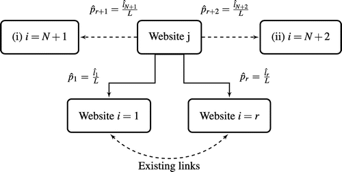
Another modification of the Google algorithm allows us to take network growth roughly into account. For this, let L be the number of users on the website j, and suppose that there are r direct links from this site to pages . The users follow the links independently of each other. Suppose further, that there are two additional possibilities for the users: (i) they can leave the known internet completely, or (ii) they can proceed to a site that is not yet ranked by the search engine (i.e., to a very recently appeared website). One can consider possibilities (i) and (ii) as dummy links N + 1 and N + 2 from the site (Figure 4). Note that the number of dummy nodes can be chosen arbitrarily and that the sample space is partitioned into a disjoint union of cells. An extended multinomial model accounting for nondisjoint cells is presented by Dong and Yin (2018).
The probability that exactly li users proceed from the site j to i is
By using Stirling’s approximation, for large L and in (25), we arrive at the equation . Combined with the probability addition rule and an assumption , it results in the expression for , which can be bounded from above by . Note that the overestimation takes the smallest value at the mean of the multinomial distribution (i.e., where is at maximum). Now we can construct the jth column of an extended transition matrix of the size ; that is, .
(Power Method with the Modified Matrix )
Construct matrix , assuming equally probable transitions from the nodes N + 1 and N + 2 to any node.
Choose a starting point from the standard simplex. Set maximal number of iterations K.
for do end for
After building the transportation matrix column by column with an assumption of equally probable transitions from the dummy nodes N + 1 and N + 2 to any node in the network, one computes the dominant eigenvector. Note that the constructed matrix is nonnegative and aperiodic. Furthermore, it is irreducible, as every state in the network is accessible from every other state. Therefore, power iterations described in Algorithm 3 converge. The resulting vector can be used as a starting point in middle-size cases for the estimation of the sum , which is an important factor for the optimality gap reduction, as shown in Section 3. Furthermore, it can help to account for the network growth in huge-dimensional cases, where the use of subgradient methods is prohibited and the efficiency is of the utmost importance. In this case, due to the necessity store, maintain, and generate large amounts of data about each website (e.g., number of users and user ratio following existing links), some simplifications of Algorithm 3 can be beneficial. For example, an assumption about equally possible transitions among existing links would replace probabilities by for each website. Further, imposing in (25) would result in . Additionally, if there would be M + 1 dummy nodes, then the transition probability from a website j to any of M new pages would be equal to . In Figure 5, we use Models 1 and 2, as well as the real-world data sets Computational Complexity and Movies (see Section 5) to observe the influence of the ratio of users following existing links on the total importance of N pages and on the uncertainty budget . For this, we distort matrix P, multiplying it by , and we add rows with probabilities .
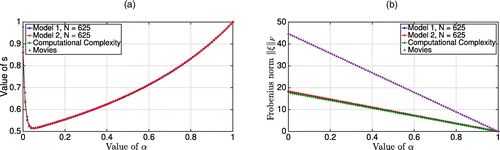
Note. (a) The total importance of N pages ; (b) the estimated uncertainty budget .
We observe that values of α close to 1 result in high values of the sum s (importance of existing pages) in Figure 5(a): α beyond 0.85 leads to s > 0.9 for all of the tested models. This is especially important, as high values of s result in lower optimality gaps, as shown in Section 8. Clearly, high values of the ratio α also imply low values of the uncertainty , which is higher for the Computational Complexity network due to its dimensionality (4,754 compared with 625 of Models 1 and 2 and 789 of the Movies data set; Figure 5(b)).
5. Data
We use both simulated and real-world data sets for the analysis of the ranking solution robust to variations in links and to the network growth. For simulated data, we use two network models introduced in the works of Timonina (2009), Polyak and Timonina (2011), and Juditsky and Polyak (2012). Using real-world data sets on link analysis ranking described in by Borodin et al. (2001), we test the proposed techniques and find implications of network growth for real-world information systems.
5.1. Simulated Data
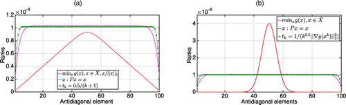
Figure 6 demonstrates two network models introduced in the works of Timonina (2009), Polyak and Timonina (2011), and Juditsky and Polyak (2012). The models are very convenient for high-dimensional analysis due to their simplified structure allowing realistic sparsity. For both models, nodes are shown as circles, while links are denoted by arrows. In Model 1, node (n, n) represents a dangling vertex, which makes the transition matrix P reducible, leading to nonuniqueness of the eigenvector corresponding to the eigenvalue λ = 1. We assume the ability of equally probable transitions from the node (n, n) to any node in Model 1 similarly to the approach used by search engines.
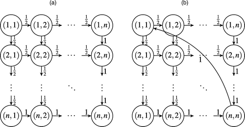
Note. (a) Model 1; (b) Model 2.
The transition matrix P corresponding to Model 1 with equally probable transitions from the vertex (n, n) becomes irreducible and aperiodic, which guarantees the uniqueness of the eigenvector corresponding to the eigenvalue λ = 1, as well as the convergence of the well-known power method (Timonina 2009, Polyak and Timonina 2011, Juditsky and Polyak 2012). The transition matrix P corresponding to Model 1 is clearly highly sparse.
Model 2 differs from Model 1, as it has only one link from the node (n, n). As the transition matrix corresponding to the Model 2 is periodic, the power method does not converge for it (Timonina 2009, Polyak and Timonina 2011).
Both models have closed-form solutions, and, therefore, the performance of numerical algorithms can be easily tested in comparison with the true ranks (Timonina 2009, Polyak and Timonina 2011). We use a standard normalization for both Model 1 and Model 2 (Figure 7). Note that the ranks correspond to the dominant eigenvector of the matrix P. However, they are not necessarily the optimal solution of the optimization Problem (20).
Note. (a) Model 1; (b) Model 2.
5.2. Real-World Data Sets
We use Computational Complexity (CompCom) and Movies (online film repositories) data sets, downloaded from http://www.cs.toronto.edu/t~sap/. CompCom data represent 789 journals on computational complexity with a total of 1,449 links, while Movies has 4,754 online film repositories and 17,198 links: transition matrices derived based on the data sets are both very sparse and suitable for our purposes. The optimal value of Problem (20) with the transition matrix implied by CompCom data and ϵ = 1 is equal to 0.0587, while the optimal value implied by the Movies data is 0.0288: these values and their corresponding solution vectors are used as benchmarks in Sections 6 and 7.
6. Convergence Results
We have performed extensive numerical analysis for the convergence of the proposed algorithms and their variations (Figures 8–12). For this, we have employed both simulated and real-world data sets. In this section, we provide the most representative convergence results.
Note. (a) Objective value; (b) number of zero ranks.
Note. (a) Google matrix G; (b) omitting the monotonicity condition.
Note. (a) Model 1; (b) Model 2.
Note. (a) Model 1; (b) Model 2.
Note. (a) Objective function; (b) distance to .
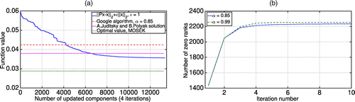
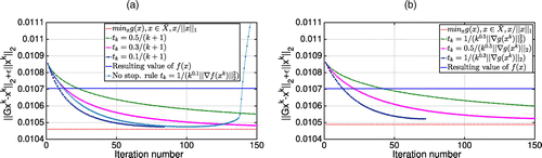
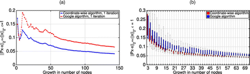
We compare a high-accuracy solution of Problem (20) computed using MOSEK optimization software with (i) the scores implied by Algorithm 1, (ii) ranks estimated by the algorithm of Juditsky and Polyak (2012), as well as with (iii) the approximation obtained by the PageRank algorithm. As expected, Algorithm 1 is monotonically decreasing in the function value of Problem (20) and provides high-quality optimal value approximation results. Figure 8 demonstrates iterations of the algorithm for the Movies data set: in Figure 8(a), one can see that the optimal value is lower than both that of the Google algorithm and of Juditsky and Polyak (2012) after four iterations; Figure 8(b) demonstrates the increasing number of zero components, making the algorithm more efficient from iteration to iteration.
As Algorithm 1 is descending with near-optimal step size, it aims for the approximation of the optimal solution of Problem (20) by reducing the objective value at each iteration. Furthermore, the value of the modified objective in (21) can be decreasing in parallel due to the choice of the subgradient (Figure 9(a)). This, however, does not imply that the monotonicity condition from Algorithm 1 can easily be omitted: neglecting this condition, one does not necessarily obtain the convergence (Figure 9(b)).
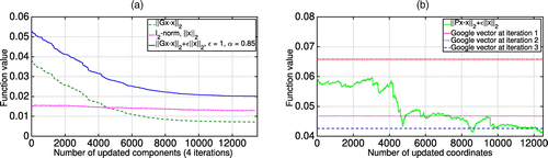
Further, we analyze the subgradient algorithm in (24) on Models 1 and 2 with N = 10,000. The subgradient method is not necessarily descending in the objective value, and we test different possible step sizes for its convergence. In Figures 10(a) and 11(a), we consider the square summable but not summable step sizes satisfying . In Figures 10(b) and 11(b), we analyze the Polyak step size of the type . We use the stopping rule in both Figures 10 and 11, and we demonstrate the performance of the algorithm without it in Figure 10(a) for the Polyak step size. Note that the stopping rule allows us to avoid keeping track of the best function value, which is less efficient.
As seen in Figure 11, the subgradient method in (24) does not distinguish between high-importance pages, similar to the Google algorithm (Polyak and Timonina 2011). Furthermore, it results in an objective value of (20) equal to approximately 0.0107, which is approximately 5% higher than the value provided by Algorithm 1, that is, 0.0102 in Figure 12(a).
Next, we test Algorithms 1–3 on Model 2 with N = 10,000 in Figure 12. As expected, Algorithm 1 results in the smallest objective value of (20). The vector minimizing (20) corresponds to the ranking that is robust to network perturbations in size and in structure. Importantly, comparing the solutions of Algorithms 1–3 with the dominant eigenvector of matrix P in Figure 12(b), we observe that the robust vector has the largest l2-distance to . Indeed, the larger the parameter ϵ, the further the two vectors are. Overall, Algorithm 1 is suggested for the computation of the robust vector in middle-dimensional cases due to its accuracy. In high dimensions, the robust vector can be approximated using Algorithms 2 and 3, as well as the Google algorithm. In this case, the robustness holds for small values of ϵ and regular matrices P (Juditsky and Polyak 2012): the conditions that guarantee the proximity of the true solution to .
In general, the problem of computing the dominant eigenvector of P is different from the problem of finding the robust ranking. In order to recover the dominant eigenvector of the unperturbed matrix P in high dimensions, one can implement fast iterative algorithms using a sequence of transition matrices converging to P. Such iterative regularization schemes are discussed in the works of Timonina (2009), Polyak and Timonina (2011), and Juditsky and Polyak (2012), and they remind methods for solving variational inequalities are discussed in the work of Bakushinskij and Polyak (1974).
7. Implications for Information Systems
Using the real-world data sets Movies and CompCom, we analyze the impact of the network growth on ranking. The network Movies contains 4,754 web repositories for films, while the data set CompCom contains 789 journals on computational complexity. As there is no historical data on when the nodes (i.e., movie repositories or journals) are created, we consider multiple growth paths by selecting random submatrices of increasing dimension from the transportation matrix. Afterward, we use both the Google algorithm and our Algorithm 1 to obtain ranking vectors for the networks. Figure 13 demonstrates that, already after the first iteration, Algorithm 1 provides a finer approximation for the robust vector as compared with the Google algorithm. This is true for all the growth values except very low ones, for which both methods perform similarly (Figure 13(a)). Furthermore, the objective value obtained via Algorithm 1 is lower for each surplus in the number of nodes, not only for a particular path in Figure 13(a), but also for the average among 100 random growth trajectories in Figure 13(b).
Note. (a) One possible path; (b) average among 100 paths.
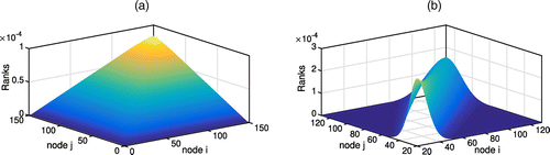
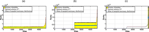
Next, comparing ranking vectors estimated via different methods with the true robust ranking obtained via MOSEK software, we see that both the Google algorithm and the algorithm of Juditsky and Polyak (2012) underestimate ranks of high-importance pages and neglect the clustering effect, which can be observed for the true ranks (Figure 14, (a), (b), and (d)). We also observe that the vector robust to the network growth does not coincide with dominant eigenvectors of G or P (Figure 14, (a) and (d)). Thus, the robust vector cannot be found simply by power iterations. Also, one cannot apply the highly efficient algorithms proposed in Polyak and Timonina (2011).
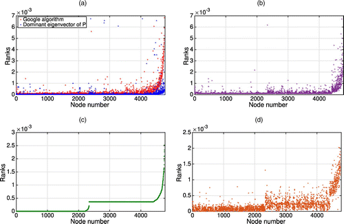
Note. (a) Dominant eigenvectors; (b) Juditsky and Polyak algorithm; (c) Algorithm 1; (d) MOSEK algorithm.
Figure 14(c) demonstrates the ranking obtained via Algorithm 1. The ranking vector clearly distinguishes between three groups of nodes: (i) high-importance nodes, (ii) nodes of medium importance, and (iii) unimportant nodes receiving zero ranks. This corresponds to the clustering observed for the true ranks in Figure 14(d). Similar effects can be observed for the CompCom data set.
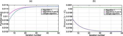
Using the Movies data set, the optimal value of Problem (20) is 0.0288. After four iterations, the approximate solution supplied by Juditsky and Polyak (2012) attains the value 0.0379; Algorithm 1 provides the vector with the function value 0.0356, while the Google algorithm results in 0.0424. Thus, Algorithm 1 results in a 6% improvement compared with the solution of Juditsky and Polyak (2012) and in 16% improvement compared with the Google algorithm. In the CompCom experiment, the optimal value of Problem (20) is 0.0587. The corresponding value for the solution supplied by Juditsky and Polyak (2012) (after three iterations) is 0.0756. Algorithm 1 provides the vector with the function value 0.0703, while the Google algorithm results in 0.0814. The percentage improvements are 7% and 14%, respectively.
Lemma 1 and Statement 1 play an important role here. They allow us to claim which of the estimated vectors are robust to the network growth via computing the values for the uncertainty parameters satisfying the robustness. Similar to Figure 1, Figure 15 demonstrates the areas where the estimated ranks are robust to variations in links and to the network growth and where the robustness is not validated. We observe that, for (i.e., for all feasible values of uncertainty), the vector obtained via Algorithm 1 satisfies the robustness criterion in (13) at a 15% growth rate (Figure 15(a)). However, the Google vector is not robust to variations in links and to the same growth in the number of nodes for a large portion of uncertainty parameters (Figure 15(b)). For example, the Google vector does not satisfy robustness criteria for the network with 260 nodes and uncertainty at 15% expected growth. Furthermore, the objective function value corresponding to the vector supplied by Algorithm 1 can be much lower than the value corresponding to the Google vector (see Figure 11). Thus, Algorithm 1 provides a finer approximation of the robust ranking vector than the Google algorithm.
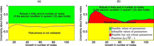
Note. (a) Algorithm 1; (b) Google algorithm.
8. Numerical Analysis of the Approximation Quality
In this section, we numerically assess the approximation quality of our methods. Invoking Corollary 1, we have a theoretical foundation to bound the optimality gap given the total importance of current pages . We denote this bound by v(s). Importantly, the optimality gap between Problems (5) and (8) can be bounded by v(s) if the value of s is underestimated with respect to the true importance of current pages ; that is, if (see Online Appendix A.5). Conversely, if the importance s is overestimated, that is, if , then the true optimality gap can be bounded by a value in some distance δv to v(s). The value of δv would converge to zero in the number of new pages M if the value of the uncertainty parameter would stay constant. This, however, is not the case due to the conditions of Corollary 1.
Overall, the optimality gap between Problems (5) and (8) can be bounded in line with Inequality in Online Appendix A.5, for which the condition of Lemma 1 (point 1) should hold. Its lowest value is suggested for high growth rates M.
Further, we consider pessimistic and optimistic scenarios, which we distinguish in terms of over- or underestimation of the optimality gap given the total importance of current pages s.
Pessimistic Scenario.
We use Propositions 1 and 2 and guarantee that and . Thus, the optimality gap is overestimated. We refer to this case as the pessimistic one.
Optimistic Scenario.
We relax the lower bounds in Propositions 1 and 2, allowing perturbation matrices ξ and ψ to take values outside of the feasibility region , keeping the column-stochasticity constraints only. As the optimality gap can be underestimated via this approach, we refer to this case as the optimistic one.
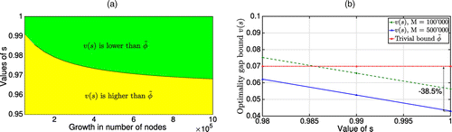
In both scenarios, we search for such values of s that lead to (Figure 16 for the optimistic case using Propositions 1). Otherwise, the trivial bound is stronger than the bound imposed by Corollary 1.
Notes. (a) Values of s. (b) Gap reduction.
Further, we consider the boost growth setup, in which we require (Figure 16(b)). We analyze the behavior of the optimality gap bounds for the case when ϵ2 depends on M, as required by Corollary 1. Specifically, we impose , and , which implies that new pages do not give a part of their possible rank to current pages. By this, we satisfy the conditions of Corollary 1, using minimal possible values for the analysis. We also take into account that only the sum plays a role for the value of the optimality gap in (A18) and in Problem (8). Additionally, stress-tests our ranking approach, as dangling vertices imply the reducibility of the transition matrix Q (Polyak and Timonina 2011).
Figures 2, 3, and 17 refer to the pessimistic scenario. In Figure 17(a), we consider the overestimated total importance of current pages s = 1 and observe the convergence of the ratio of two upper bounds for the optimality gap in the number of new pages M. The convergence is not to zero due to the dependency of the uncertainty parameter ϵ2 on M, as suggested in Online Appendix A.5.
Note. (a) Convergence, ; (b) bound v(s); (c) bound (A18).
We observe that Proposition 1 leads to an approximately 5% lower value for v(1) compared with the bound in the boost growth case. The bound increases in relative terms if the total importance of current pages s decreases (Figure 17(b)).
Moreover, overestimating by s = 1 in Figure 17(c), we bound the optimality gap in line with Inequality (A18) and demonstrate the area where it belongs with yellow. Importantly, the resulting bound appears to be stronger than the bound estimated via the use of Proposition 1. This depends on the chosen set of parameters and follows from the fact that , (Section 3 and Online Appendix A.5).
Further, Figure 18 demonstrates the dependency of the optimistic optimality gap on uncertainty parameters and in the boost growth setup. By solving the optimization Problem (20) for given and , we generate matrices ξ and ψ, so that Q stays column-stochastic, and compute the value in Proposition 1. We show the estimate in absolute and in relative terms in Figure 18, (a) and (b), respectively. In Figure 18(a), we see that larger uncertainty parameters clearly lead to higher gaps in absolute terms. Similar to Figure 3 for the pessimistic case, we observe an asymmetrical behavior suggesting the largest gap reduction for low values of the parameter and high values of (Figure 18(b)). Compared with the maximal reduction of approximately 30% in Figure 18(b), the maximal reduction achieved by Proposition 2 is approximately 15%.
Note. (a) Optimistic scenario; (b) approximation ratio.
Beyond the assessment of pessimistic and optimistic scenarios, we analyze the difference in optimal solutions between the initial Problem (5) and its approximation (19) for the Movies data set (Figure 19). Using Corollary 2, we generate 10,000 pairs and verify whether they satisfy Inequality (16). We can exclude all those that do not satisfy (16) at least for one generated ξ.
Note. (a) 100% variable ranks; (b) 10% variable ranks; (c) 1% variable ranks.
Figure 19 demonstrates that the ranks of current pages start equalizing on average as a result of an increase in uncertainty levels. For this, we suppose that 100%, 10%, or 1% of high ranks are overestimated. The score equalization would also be the result of an increase in the uncertainty parameter (Juditsky and Polyak 2012). Importantly, the only point that definitely satisfies (16) for all perturbation matrices ξ is our robust solution .
9. Conclusion
The World Wide Web is constantly changing: the amount of information on the web is growing, new pages appear, and some websites (old or spam ones) disappear. According to the Web Server Survey, the average speed of internet growth is around 1%–3% per month. The initial idea of the PageRank algorithm is based on the interchange of ranks between web pages in line with probability theory rules and results in a ranking that does not account for the rapid growth of the network and, furthermore, is not necessarily unique. In early works on the topic, the original problem is replaced with finding the principal eigenvector of a modified matrix with only positive components to impose uniqueness of the solution in the PageRank formulation. The modified matrix assumes direct transitions between pages, which do not have direct links between one another is known as the Google matrix and is broadly used in practice. However, the principal eigenvector may be significantly influenced by this difference in matrices, and, importantly, for specific network structures, the eigenvector of the Google matrix may stop distinguishing between high-ranked pages that build the core of search engine results. In this article, we account for the uncertainty in the transition matrix, and we formulate the internet ranking problem as an optimization problem robust to variations in links and to the network growth.
We propose an l2-norm robust reformulation of the PageRank problem for uncertain networks with fixed growth rates, and we bound this reformulation from above by a separable convex but nonsmooth optimization problem. The separability of the upper bound plays a crucial role for the robustness: one can conclude under which conditions on the uncertainty about future pages the estimated ranking is robust to variations in links and in the network structure and under which conditions it is not. We test the robustness of the Google vector, the ranking proposed by Juditsky and Polyak, and the ranking obtained via our algorithm.
We demonstrate that the formulation robust to network growth imposes an upper bound on the l2-norm formulation robust to perturbations solely in links. We consider smoothing techniques for the subgradient method, avoiding all nonsmooth points, in order to solve the formulated optimization problem in middle-dimensional cases via a coordinate-wise descent method with near-optimal step size. We also address high-dimensional cases and propose two variations of the Google algorithm. Their performance depends on the unperturbed network structure and, thus, on the context of application. This provides a variety of opportunities for future research. In this article, we use simulated data and the real-world data sets Movies and CompCom to analyze our algorithms and assess the impact of the network growth on ranking.
By assessing the approximation quality from both theoretical and numerical perspectives, we observe that the optimality gap takes its smallest value in case of a rapid growth in the number of pages, while the size of the optimality gap reduction depends on the total importance of current pages. Also, we demonstrate a case when the optimality gap takes zero value: this happens given a specific structure of the uncertainty matrix.
The PageRank problem has a wide range of possible applications (Agarwal and Venkatesh 2002; Pant and Srinivasan 2010, 2013; Xu et al. 2011; Sundararajan et al. 2013; Dhar et al. 2014; Zhu et al. 2014; Pant and Sheng 2015; Van Vlasselaer et al. 2017; Shah et al. 2020). From theoretical and numerical perspectives, future research can focus on different types of structural perturbations of transition matrices (Juditsky and Polyak 2012) and randomized techniques for the computation of the robust stationary distribution in high-dimensional cases (Polyak 2001, Polyak and Tempo 2001, Nazin and Polyak 2009, Bomze et al. 2021).
The authors thank the area editor, Prof. John Birge, the associate editor, and the anonymous reviewers for their thoughtful comments and efforts toward improving our manuscript. Last but not least, we are grateful to Prof. Daniel Kuhn at École Polytechnique Fédérale de Lausanne for his very valuable remarks about the approximation quality.
References
- (2002) Assessing a firm’s web presence: A heuristic evaluation procedure for the measurement of usability. Inform. Systems Res. 13(2):168–186.Link, Google Scholar
- (2002) Developing and validating an instrument for measuring user-perceived web quality. Inform. Management 39(6):467–476.Crossref, Google Scholar
- (1974) On the solution of variational inequalities. Soviet Math. Doklady 14:1705–1710.Google Scholar
- (2017) First-Order Methods in Optimization (SIAM, Philadelphia).Crossref, Google Scholar
- (2012) Smoothing and first-order methods: A unified framework. SIAM J. Optim. 22(2):557–580.Crossref, Google Scholar
- (1998) Robust convex optimization. Math. Oper. Res. 23(4):769–805.Link, Google Scholar
- (2021) Trust your data or not—StQP remains StQP: Community detection via robust standard quadratic optimization. Math. Oper. Res. 46(1):301–316.Link, Google Scholar
- (2004) Convex Optimization (Cambridge University Press, Cambridge, UK).Crossref, Google Scholar
- (2018) Introduction to Applied Linear Algebra: Vectors, Matrices, and Least Squares (Cambridge University Press, Cambridge, UK).Crossref, Google Scholar
- (2001) Finding authorities and hubs from link structures on the World Wide Web. Proc. 10th Internat. World Wide Web Conf. (ACM, New York).Google Scholar
- (1998) The anatomy of a large-scale hypertextual web search engine. Comput. Networks ISDN Systems 30(1–7), 107–117.Crossref, Google Scholar
- (2006) The $25,000,000,000 eigenvector: The linear algebra behind Google. SIAM Rev. 48(3):569–581.Crossref, Google Scholar
- (2020) A dynamic network model of interbank lending—systemic risk and liquidity provisioning. Math. Oper. Res. 45(3), 1127–1152.Link, Google Scholar
- (2016) An optimization view of financial systemic risk modeling: Network effect and market liquidity effect. Oper. Res. 64(5):1089–1108.Link, Google Scholar
- (2017) Optimizing click-through in online rankings with endogenous search refinement. Marketing Sci. 36(4):542–564.Link, Google Scholar
- (2014) Prediction in economic networks. Inform. Systems Res. 25(2):264–284.Link, Google Scholar
- (2018) Maximum likelihood estimation for incomplete multinomial data via the Weaver algorithm. Statistics Comput. 28:1095–1117.Crossref, Google Scholar
- (2011) PageRank: Standing on the shoulders of giants. Comm. ACM 54(6):92–101.Crossref, Google Scholar
- (2003) The second eigenvalue of the Google matrix. Technical report, Department of Computer Science, Stanford University.Google Scholar
- (1990) Matrix Analysis (Cambridge University Press, Cambridge, UK).Google Scholar
- (2010) Distributed randomized algorithms for the PageRank computation. IEEE Trans. Automatic Control 55(9):1987–2002.Crossref, Google Scholar
- (2005) Randomized algorithms for synthesis of switching rules for multimodal systems. IEEE Trans. Automatic Control 50(6):754–767.Crossref, Google Scholar
- (2012)
First order methods for nonsmooth convex large-scale optimization, II: Utilizing problems structure . Sra S, Nowozin S, Wright S, eds. Optimization for Machine Learning (MIT Press, Cambridge, MA), 121–184.Google Scholar - (2012) Robust eigenvector of a stochastic matrix with application to PageRank. Proc. 51st IEEE Conf. Decision Control (IEEE, Piscataway, NJ), 3171–3176.Google Scholar
- (2012) Validation analysis of mirror descent stochastic approximation method. Math. Programming 134(2):425–458.Crossref, Google Scholar
- (2006) Google’s PageRank and Beyond: The Science of Search Engine Rankings (Princeton University Press, Princeton, NJ),Crossref, Google Scholar
- (2019) Bibliometric analysis for highly cited papers in operations research and management science from 2008 to 2017 based on essential science indicators. Omega 88:223–236.Crossref, Google Scholar
- (2004) Deeper inside PageRank. Internet Math. 1(3):335–380.Crossref, Google Scholar
- (2016) The impact of fake reviews on online visibility: A vulnerability assessment of the hotel industry. Inform. Systems Res. 27(4):940–961.Link, Google Scholar
- (2014) Distributed randomized PageRank algorithm based on stochastic approximation. IEEE Trans. Automatic Control 60(6):1641–1646.Crossref, Google Scholar
- (2009) Adaptive randomized algorithm for finding eigenvector of stochastic matrix with application to PageRank. Proc. Joint 48th IEEE Conf. Decision Control 28th Chinese Control Conf. (IEEE, Piscataway, NJ), 127–132.Google Scholar
- (2017) Rank centrality: Ranking from pairwise comparisons. Oper. Res. 65(1):266–287.Link, Google Scholar
- (2004) Prox-method with rate of convergence O(1/t) for variational inequalities with Lipschitz continuous monotone operators and smooth convex-concave saddle point problems. SIAM J. Optim. 15(1):229–251.Crossref, Google Scholar
- (1983) Problem Complexity and Method Efficiency in Optimization (Wiley, New York).Google Scholar
- (2005) Smooth minimization of non-smooth functions. Math. Programming 103(1):127–152.Crossref, Google Scholar
- (2007) Dual extrapolation and its applications to solving variational inequalities and related problems. Math. Programming 109(2–3):319–344.Crossref, Google Scholar
- (2014) Subgradient methods for huge-scale optimization problems. Math. Programming 146(1–2):275–297.Crossref, Google Scholar
- (1998) The PageRank citation ranking: Bringing order to the web. Technical report, Stanford Digital Library Technologies Project, Stanford University.Google Scholar
- (2002) Website usability, design, and performance metrics. Inform. Systems Res. 13(2):151–167.Link, Google Scholar
- (2010) Predicting web page status. Inform. Systems Res. 21(2):345–364.Link, Google Scholar
- (2013) Status locality on the web: Implications for building focused collections. Inform. Systems Res. 24(3):802–821.Link, Google Scholar
- (2015) Web footprints of firms: Using online isomorphism for competitor identification. Inform. Systems Res. 26(1):188–209.Link, Google Scholar
- (1987) Introduction to Optimization (Optimization Software Publications, New York).Google Scholar
- (2001)
Random algorithms for solving convex inequalities . Butnariu D, Censor Y, Reich S, eds. Inherently Parallel Algorithms in Feasibility and Optimization and Their Applications (Elsevier, Amsterdam), 409–422.Crossref, Google Scholar - (2001) Probabilistic robust design with linear quadratic regulators. Systems Control Lett. 43(5):343–353.Crossref, Google Scholar
- (2011) PageRank: New regularizations and simulation models. IFAC Proc. Vol. 44(1):11202–11207.Google Scholar
- (2015) Measuring systemic risk: Robust ranking techniques approach. Preprint, submitted March 21, https://doi.org/10.48550/arXiv.1503.06317.Google Scholar
- (2020) Adaptive matching for expert systems with uncertain task types. Oper. Res. 68(5):1403–1424.Link, Google Scholar
- (2013) Research commentary-information in digital, economic, and social networks. Inform. Systems Res. 24(4):883–905.Link, Google Scholar
- (1996) Regression shrinkage and selection via the lasso. J. Royal Statist. Soc. B 58(1):267–288.Crossref, Google Scholar
- (2009) The rank-model and its investigations (in Russian). Stochastic Optim. Informatics 5:139–156.Google Scholar
- (2017) Gotcha! Network-based fraud detection for social security fraud. Management Sci. 63(9):3090–3110.Link, Google Scholar
- (2011) Evaluating OR/MS journals via PageRank. Interfaces 41(4):375–388.Link, Google Scholar
- (2020) Content growth and attention contagion in information networks: Addressing information poverty on Wikipedia. Inform. Systems Res. 31(2):491–509.Link, Google Scholar
- (2014) Scheduled service network design for freight rail transportation. Oper. Res. 62(2):383–400.Link, Google Scholar
Anna Timonina-Farkas is a scientific researcher at École Polytechnique Fédérale de Lausanne conducting fundamental and applied research in the field of operations research and operations management. Her focus is on theory and data-driven solution methods in multi-stage optimization under model and decision-dependent uncertainties. She has received several awards for the quality of her research, including the University of Vienna Publication Award (2017) and a Schrödinger Fellowship (2015).
Ralf W. Seifert is a professor of technology and operations management at École Polytechnique Fédérale de Lausanne. He also holds a professorship in operations management at the International Institute for Management Development. His primary research and teaching interests relate to operations management, supply chain strategy, and technology network management.

