


Dynamic Demand Management for Parcel Lockers
Abstract
In pursuit of a more environmentally sustainable and cost-efficient last mile, parcel lockers have gained a firm foothold in the parcel delivery landscape. To fully exploit their potential and ensure customer satisfaction, successful management of the locker’s limited capacity is crucial. This is challenging as future delivery requests and pickup times are stochastic from the provider’s perspective. In response, we propose to dynamically control whether the locker is presented as an available delivery option to each incoming customer with the goal of maximizing the number of served requests. We take compartment sizes into account, which entails a second type of decision as parcels scheduled for delivery must be allocated. As an extension, we balance rejected requests and failed deliveries through a careful use of overbooking. We formalize the problem as an infinite-horizon sequential decision problem and find that exact methods are intractable for realistic instances. In light of this, we develop a solution framework that orchestrates multiple algorithmic techniques from sequential decision analytics and reinforcement learning in an innovative way, namely cost function approximation and value function approximation (VFA). As a general methodological contribution, we enhance the training of our VFA with a modified version of experience replay. Our computational study shows that our method outperforms a myopic benchmark by 3.4% and an industry-inspired policy by 2.8%.
Supplemental Material: The online appendices are available at https://doi.org/10.1287/trsc.2024.0871.
1. Introduction
Parcel lockers have evolved into a viable alternative to traditional home delivery and are gaining increasing popularity worldwide. Recent surveys show, for example, that 54% of online shoppers in Poland prefer to receive their parcels via parcel lockers (DHL 2022), 57% in China (Statista 2022), and in Estonia, 70% favor parcel lockers over other delivery options, such as home delivery (Venipak 2023). Because these lockers offer a huge potential to consolidate deliveries and decrease failed delivery attempts (Savelsbergh and Van Woensel 2016), this is an encouraging development in the quest for a green and cost-efficient last mile.
In this context, parcel recipients play a pivotal role in two ways: On the one hand, their purchasing habits and location preferences shape the number of incoming delivery requests because recipients usually select a specific locker as the desired delivery address in practice. Generally, recipients tend to prefer lockers that are close to their home or that can be easily integrated into regular trips, for example, the commute to work. On the other hand, the speed at which recipients pick up their parcel directly affects the available capacity over time. As a result, recipients’ behavior creates two sources of uncertainty from a locker operator’s perspective.
Because of these stochastic influences, parcel lockers are susceptible to short-term mismatches between capacity and demand. Typically, a locker consists of individual compartments of different sizes. This introduces compatibility constraints as the compartment assigned to a parcel must be large enough. The total number of compartments per size and thus the locker’s capacity is fixed in the short term. By contrast, the availability of compartments over time is stochastic because it depends on how fast recipients collect their parcels.
In reality, it may regularly occur that parcels cannot be delivered to the locker chosen by the recipient because all compatible compartments are already occupied. As a widespread strategy, companies redirect parcels to another locker in such cases. However, this may leave the recipient very dissatisfied, especially if picking up their parcel from the alternative locker requires a large detour. Furthermore, depending on the business model, recipients can be grouped according to their pickup behavior (Sethuraman et al. 2024). If the parcels of fast-collecting customers tend to arrive on short notice (e.g., because of express shipping), the problem is exacerbated as they might get redirected disproportionately often.
Consequently, we advocate for actively managing scarce locker capacity instead of merely handling capacity shortages in a reactive way. To accomplish this, we propose to dynamically control the availability of the parcel locker as a delivery option for each incoming request. We call the resulting problem the dynamic parcel locker demand management problem (DPLDMP). For ease of exposition, we refer to the decision maker as a general “provider” and use the terms “customer” and “recipient” synonymously.
More specifically, the DPLDMP can be summarized as follows: We focus on a single parcel locker and assume that parcels are delivered to the locker once per day. The locker consists of multiple compartments that differ in their size. The availability of compartments over time depends on the customers’ pickup behavior and is uncertain. Over the course of each day, requests arrive stochastically. For each incoming request, the provider determines whether a suitable compartment will be available. Subsequently, the provider makes a demand control decision, that is, decides whether to accept or reject the request. In the case of acceptance, the request turns into an order and the associated parcel has to be delivered to the locker on its given delivery date. If the provider rejects the request, the customer gets informed that the parcel locker is currently not available as a delivery option. The customer might then choose another option such as home delivery or an alternative parcel locker, which is outside of our paper’s scope. At the end of each day, the provider assigns parcels scheduled for delivery on the following day to available compartments, which we refer to as the allocation decision. The overall goal is to maximize the expected number of successful deliveries.
Because of the stochastic influences and dynamic decision making, the DPLDMP is an infinite-horizon sequential decision problem. Finding a good policy for it is difficult for two main reasons.
Two decision types. In our problem, the provider has to make two types of nontrivial decisions at different points in time. These decisions are heavily intertwined: Demand control determines which requests turn into orders and must be allocated to compartments later on. In the same vein, allocation decisions affect which compartments are occupied, thereby shaping the decision space for future demand control.
Displacement effects. Accepting a request yields an immediate reward as the number of accepted requests increases. At the same time, the available capacity decreases. Similarly, an inefficient allocation of parcels to compartments can impair demand control. Both decision types thus entail displacement effects that one has to anticipate and, in the case of demand control, trade off with the immediate reward. These effects are hard to estimate because future incoming requests and capacity consumption are uncertain.
To address these challenges, we develop a solution framework that combines and orchestrates multiple techniques from sequential decision analytics (Powell 2022) and reinforcement learning (RL; Sutton and Barto 2018). At its core, we employ cost function approximation (CFA) for the allocation decision and an offline trained parametric value function approximation (VFA) for demand control. Applying these methods to the DPLDMP is not straightforward. Notably, our approach needs to cope with two types of strongly entangled decisions at different points in time. To achieve this, we design the CFA such that it prioritizes creating favorable conditions for demand control. For the VFA, we incorporate uncertain pickups and anticipated allocation decisions in a tentative allocation plan, which forms the basis for our features. As a result, we take into account the impact of one decision type on the other and vice versa. To enable overbooking, that is, the acceptance of possibly infeasible requests, we extend our framework by artificially inflating the locker capacity when checking feasibility. We derive this virtual capacity with Bayesian optimization (BO).
With our work, we contribute to the literature in the following ways:
To the best of our knowledge, we are the first to consider demand management for parcel lockers with multiple compartment sizes and formalize it as a sequential decision problem.
We propose an anticipatory solution framework that handles two types of decisions at different points in time in an infinite horizon. Importantly, we explicitly address the strong interrelations between the decision types by combining different algorithmic techniques such as CFA and VFA in a novel way.
As a general methodological contribution, we augment an existing temporal difference learning method using the principle of experience replay to learn the weights for the VFA and stabilize the learning process.
We extend our model and solution approach with a static virtual capacity to enable overbooking.
In our computational study, we present key insights into the DPLDMP gained from a structural characterization of the optimal policy and managerial analyses on customer heterogeneity and overbooking.
The remainder of this paper is structured as follows: In Section 2, we review the literature related to the DPLDMP and highlight the resulting research gap. In Section 3, we provide a detailed problem description along with a discussion of key assumptions and model the DPLDMP as a sequential decision problem. In Section 4, we propose our solution framework. We present the results of our computational study in Section 5 and conclude the paper with future research directions in Section 6.
2. Related Work
In this section, we give a concise review of the three major literature streams related to the DPLDMP. Section 2.1 focuses on demand management for out-of-home delivery, thereby covering publications in a similar application context. Taking on a more theoretical perspective, Section 2.2 is dedicated to demand management with reusable resources, and Section 2.3 addresses upgrades. We summarize our findings with a tabular overview and a delineation from the most closely related work in Section 2.4.
2.1. Demand Management for Out-of-Home Delivery
The last leg of the parcel delivery process, also known as the last mile, is notoriously cost-intensive, incentivizing researchers and practitioners to innovate. This manifests itself in two key trends. First, demand management has been integrated into various existing logistics services, such as attended home delivery or same-day delivery, in recent years (Fleckenstein, Klein, and Steinhardt 2023). By controlling the availability or prices of delivery options, providers can actively steer demand (Waßmuth et al. 2023). Second, various novel delivery concepts have emerged (Boysen, Fedtke, and Schwerdfeger 2021). A prominent example is out-of-home delivery (OOHD), that is, the delivery to parcel lockers or parcel shops instead of the recipient’s home address. The DPLDMP is directly at the intersection of these two trends.
The review by Janinhoff et al. (2024) documents a surge in publications on OOHD, especially for location planning and routing problems. By contrast, research on demand management for OOHD is still in its nascent stage. Although there is work on the satisfaction of customer preferences on an aggregate level (Dumez, Lehuédé, and Péton 2021) and OOHD product design (Janinhoff, Klein, and Scholz 2023), our analysis focuses on publications that explicitly take into account operational demand management, thereby also excluding work on dynamic OOHD problems without any demand steering component (Ulmer and Streng 2019). To the best of our knowledge, there exist only three publications matching these criteria: At the start of a retailer’s fulfillment planning phase, Galiullina et al. (2024) offer selected recipients a monetary incentive to switch to OOHD by solving a two-stage stochastic program with an exact branch-and-bound algorithm as well as heuristics. Intervening at an earlier stage, Akkerman, Dieter, and Mes (2025) investigate joint availability control and dynamic pricing of delivery options during the order arrival phase for a single delivery day based on approximated delivery costs predicted by machine learning. In cooperation with retailer Amazon, Sethuraman et al. (2024) study availability control for a parcel locker with uniform compartments and employ a linear program as a lookahead model with predicted demand and pickups.
2.2. Reusable Resources
Structurally, the DPLDMP can be cast as a revenue management problem with reusable resources. In a setting with reusable resources, customers arrive dynamically and, in case of a purchase, make use of a resource for a certain (potentially stochastic) amount of time. Afterward, the resource returns to the seller and can thus be allocated several times during the planning horizon. For parcel lockers, resources correspond to the compartments, and the usage duration is stochastic because it depends on the recipient’s pickup speed. Moreover, there are different compartments sizes, that is, multiple types of resources, and delivery requests typically arrive before the actual delivery. We focus on publications that match our problem setting closely, that is, stochastic usage durations in combination with (a) multiple resource types or (b) advance reservations.
Multiple resource types.
Püschel et al. (2015) investigate rule-based dynamic pricing and availability control for a cloud-computing provider. Jointly controlling availability and prices, Owen and Simchi-Levi (2018) construct policies from linear programs serving as lookahead models. Rusmevichientong, Sumida, and Topaloglu (2020) combine a static policy with a rollout to obtain a dynamic policy that takes the current resource utilization into account. Gong et al. (2022) prove that under certain assumptions, a simple myopic policy earns at least half the expected revenue of a clairvoyant benchmark. Baek and Ma (2022) generalize availability control to a network setting and compute bid prices with approximate dynamic programming.
Advance reservations.
Papier and Thonemann (2010) propose an anticipatory policy for availability control that harnesses event probabilities computed under simplified assumptions.
2.3. Upgrading
If alternatives can be ordered in a hierarchy, a seller can make use of upgrading by satisfying the demand for a specific product with another product higher in the hierarchical order. This enables the seller to alleviate short-term mismatches between capacity and demand. In the context of parcel lockers, this mechanism is relevant due to the compartment sizes, that is, a parcel can be “upgraded” to a larger compartment size.
Out of the corresponding literature stream, we focus on publications with full cascading upgrades, that is, upgrades to any product higher in the hierarchical order. Given that the resulting papers exhibit largely identical characteristics with regard to our classification scheme in Section 2.4, we center the discussion around three representative publications and refer the interested reader to the review by Gönsch (2020). Gallego and Stefanescu (2009) analytically investigate and compare different upgrade mechanisms and incorporate fairness considerations. Gönsch and Steinhardt (2015) apply availability control with upgrades to an airline network using dynamic programming decomposition and show certain monotonicity properties of opportunity cost. In a recent publication, Zhu and Topaloglu (2024) derive an approximation of the value function to control the availability of flexible products, which are a generalization of upgrades.
2.4. Summary and Research Gap
Table 1 summarizes the literature related to the DPLDMP. We characterize the publications according to the following dimensions: Column “Decision” indicates the demand management lever (availability control (AV) or pricing (P)). The next five columns track whether the problem features multiple types of resources, upgrading, advance reservations, stochastic usage durations, and an infinite planning horizon. The last column classifies the solution approach as myopic (M) or anticipatory (A). As a special case of the latter, we highlight papers drawing on the deterministic linear program (DLP) or its choice-based variant (CDLP) because this is a fundamental revenue management concept (Gallego and Topaloglu 2019). The core idea is to construct a lookahead model where demand is assumed to take on its expected value. Heuristics then build on the primal (e.g., by comparing objective values) or dual solution (e.g., to derive bid prices).
|

Table 1. Related Literature
| Publication | Decision | Multiple resources | Upgrades | Advance reservations | Stochastic duration | Infinite horizon | Solution concept | |
|---|---|---|---|---|---|---|---|---|
| OOHD | Akkerman, Dieter, and Mes (2025) | AV, P | ✓ | ✓ | A | |||
| Galiullina et al. (2024) | P | ✓ | A | |||||
| Sethuraman et al. (2024) | AV | ✓ | ✓ | ✓ | DLP | |||
| Reusable | Baek and Ma (2022) | AV | ✓ | ✓ | CDLP | |||
| Resources | Gong et al. (2022) | AV | ✓ | ✓ | M | |||
| Owen and Simchi-Levi (2018) | AV, P | ✓ | ✓ | ✓ | CDLP | |||
| Papier and Thonemann (2010) | AV | ✓ | ✓ | ✓ | A | |||
| Püschel et al. (2015) | AV, P | ✓ | ✓ | A | ||||
| Rusmevichientong, Sumida, and Topaloglu (2020) | AV, P | ✓ | ✓ | A | ||||
| Upgrading | Gallego and Stefanescu (2009) | AV, P | ✓ | ✓ | ✓ | DLP | ||
| Gönsch and Steinhardt (2015) | AV | ✓ | ✓ | ✓ | DLP | |||
| Zhu and Topaloglu (2024) | AV | ✓ | ✓ | ✓ | A | |||
| Our work | AV | ✓ | ✓ | ✓ | ✓ | ✓ | A |
Note. A, anticipatory; AV, availability control; CDLP, choice-based deterministic linear program; DLP, deterministic linear program; M, myopic; P, pricing.
In line with the reviews by Ma, Wong, and Teo (2022) and Janinhoff et al. (2024), we find that demand management in OOHD is an emerging topic addressed by only a handful of recent publications. For all of them, a major line of distinction to our work is how capacity is modeled. Galiullina et al. (2024) assume uncapacitated facilities, whereas Akkerman, Dieter, and Mes (2025) and Sethuraman et al. (2024) consider capacitated lockers with uniform compartments. In contrast, we take into account multiple compartment sizes, thereby modeling capacity on a more granular and realistic level.
Although problems similar to the DPLDMP have been covered in the context of reusable resources or upgrading, our analysis reveals a substantial research gap. To the best of our knowledge, our work is the first to jointly consider upgrading and stochastic usage durations. Note that upgrading introduces an additional decision compared with papers that only include stochastic usage durations as customers need to be allocated to a specific resource type. Vice versa, papers that do take upgrading into account lack the stochastic usage duration that is central to OOHD due to the recipients’ pickup behavior. Our work fills this gap and may also be relevant to other application domains, for example, to manage the demand for parking lots consisting of spaces with and without charging infrastructure or station-based car sharing with multiple vehicle categories.
Concluding this section, we delineate our work from the two most closely related publications. On the one hand, the assumptions on usage durations prevent us from applying the methodology by Papier and Thonemann (2010) to the DPLDMP. Specifically, the authors do not allow for the distributions to depend on the customer type, which contradicts empirical data related to parcel lockers (Sethuraman et al. 2024). On the other hand, the DPLDMP shares strong similarities with Sethuraman et al. (2024), who use a DLP-based approach. Table 1 shows that this concept is widely used. Because we consider a novel problem at the intersection of uncertain usage durations and upgrading, we cannot directly apply any of its existing versions, but we adapt the DLP proposed by Sethuraman et al. (2024) to our problem by incorporating multiple compartment sizes and use it as a benchmark in our computational study (Section 5.1.3).
3. Problem Statement
In this section, we give a detailed description of the DPLDMP and formalize it as a sequential decision problem. Online Appendix A provides a tabular overview of the notation.
3.1. Problem Definition
In the following, we introduce the main problem components and discuss our key assumptions.
3.1.1. Description and Notation.
We define the setting of the DPLDMP as follows.
Resources.
We consider a single parcel locker. The locker consists of a limited number of compartments that differ in their size . The compartment sizes are indexed in ascending order and allow full cascading upgrades, that is, a parcel of size can be allocated to any available compartment of size . The total number of compartments per size is denoted by .
Planning horizon.
The planning horizon is divided into days . Each day is further discretized into sufficiently small time periods such that at most one request arrives per period. This yields a set of discrete points in time per day. Parcels are delivered to the locker once every day. For the allocation of parcels to compartments at the end of each day, we introduce an additional point in time with no request arrival. An entire day is thus represented by .
Requests.
The requests arrive dynamically according to a known stochastic process and are characterized by three attributes. Firstly, each request belongs to a customer type . Secondly, the parcel size indicates that the request requires a compartment of size . Thirdly, the lead time determines when the parcel must be delivered to the locker. More precisely, a parcel with lead time e has to be assigned to a compartment in the eth allocation decision from now if accepted.
Parcel pickups.
The pickup time refers to the amount of time after allocating a parcel to a compartment up until the compartment becomes available again. We express the pickup time as a tuple where b represents the number of days after allocation and the point in time at which the compartment’s status changes to unoccupied. Given that this depends on whether and when the customer collects the parcel, the pickup time is uncertain from the provider’s perspective. It follows a known distribution that may depend on the customer type c. If the customer does not collect the parcel before a specific number of days B, called the maximum storage time, elapses, the provider removes the parcel from the locker. Consequently, the maximum storage time automatically yields an upper bound on the pickup time with .
Having defined the basic setting, we elaborate on the provider’s decision making.
Feasibility check.
For each request, the provider first determines whether it is feasible. To guarantee feasibility, the decision maker must ensure that a sufficiently large compartment is going to be available from the time of delivery up until the customer picks up the parcel or the maximum storage time B elapses.
Demand control.
After the feasibility check, the provider makes a demand control decision, that is, accepts or rejects the request. In case of acceptance, the request turns into an order. If the request is rejected, the customer may choose another delivery option such as home delivery, which is out of this paper’s scope.
Allocation.
At the end of each day (), the provider allocates parcels scheduled for delivery on the following day to available and compatible compartments. Once a parcel is assigned to a specific compartment, it remains there until the customer collects it or the maximum storage time is reached.
Objective.
The provider seeks to maximize the expected number of accepted requests that result in a successful delivery.
We illustrate the sequence of decisions and events along an exemplary timeline in Figure 1.
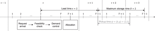
Notes. A request arrives at t on day with lead time . If the request is feasible and accepted, it has to be allocated at on day . The maximum storage time is such that the compartment assigned to the parcel is guaranteed to be available again by on . Customers usually collect their parcel earlier, leading to a specific pickup time .
3.1.2. Main Assumptions.
Our definition of the DPLDMP draws on the following assumptions.
The assumption of locker compartments allowing full cascading upgrades aligns with the locker layout configurations commonly encountered in practice. Typically, parcel lockers consist of multiple tower modules of uniform width such that the compartments sizes merely differ in their height.
For ease of exposition, one can imagine the actual delivery to the locker happening immediately after the allocation decision (for the parcels that are due for delivery on the next day). Nevertheless, our problem definition does not rely on this simplification as long as the delivery is executed once each day and roughly at the same time. We do exclude detailed operational planning such as vehicle routing and same-day delivery because it creates a highly complex setting in its own right (Ulmer and Streng 2019).
The DPLDMP focuses on last-mile logistics. In practice, parcel lockers additionally play an increasingly important role in first-mile logistics because parcel senders can also drop off their parcels (e.g., returns) at the locker. We assume that the vehicles performing the delivery to the locker have sufficient capacity to handle all dropped-off parcels upon their daily visit, allowing us to neglect first-mile logistics.
To represent the choice behavior of customers, we employ the independent demand model (Strauss, Klein, and Steinhardt 2018). In other words, we assume that every customer is interested only in one specific locker. This translates to the following process from the customer’s perspective: Each customer considering locker delivery already has a preferred locker in mind when shopping online. During the checkout process, the customer selects the desired locker through an interface, which triggers a request arrival for the provider. In case of rejection, the customer chooses another delivery option such as home delivery or abandons the purchase. The assumption of independent demand is common in the OOHD literature, particularly as the special case of customers favoring the locker closest to their home (Galiullina et al. 2024). In our case, it enables us to decompose locker networks and consider each locker independently. Although this is likely justified in sparse networks, it does neglect dynamic substitution effects that arise in denser networks where customers can easily switch to an alternative locker if their preferred one is unavailable.
We assume the size of the parcel to be known upon request arrival. As an example from practice, Amazon automatically tracks during the customer’s checkout process whether an order is eligible for delivery to a locker due to its size, weight, and other factors (Amazon 2023), rendering this assumption realistic.
The lead time is fixed, and the provider cannot pre- or postpone deliveries. While more flexibility is conceivable for a retailer, logistics service providers would have to establish intermediate storage capacities. To keep the problem relevant for as many applications as possible, we treat the lead time as given.
Empirical data show that customers with expedited shipping options tend to retrieve their parcels more quickly than those with standard shipping (Sethuraman et al. 2024). This motivates customer type–dependent distributions of pickup times. The maximum storage time is a standard concept in practice, typically ranging between three to seven days, and applies uniformly to all customer types.
For the feasibility check, we require information on the availability of compartments. This in turn hinges on the pickup times of orders currently in the locker as well as those scheduled for delivery in the next E days. Given that pickup times are uncertain, we can only guarantee a successful delivery by hedging against all possible realizations of pickup behavior. More precisely, in this strict interpretation of feasibility, we require a feasible allocation to exist even in the worst case where all customers use the maximum storage time. Note that this comes at the expense of strongly erring on the side of caution: We classify requests that can be feasibly allocated for some but not all realizations of pickup times as overall infeasible. There might thus be cases where, in hindsight, a request could have been delivered to the locker despite not passing the feasibility check. We relax this strict definition by allowing a limited use of overbooking in Section 3.4.
We do not allow parcels to be reallocated once they are assigned to a specific compartment as this would increase the operational complexity of locker deliveries.
3.2. Sequential Decision Problem
Leveraging the framework by Powell (2022), we model the DPLDMP as a sequential decision problem.
3.2.1. Decision Epoch.
A decision epoch is triggered by one of two possible events:
Request arrival. If a request arrives at , the provider makes a demand control decision.
End of day. At the end of each day, the provider has to allocate orders scheduled for delivery on the subsequent day. Consequently, a decision epoch arises whenever the system reaches .
3.2.2. Predecision State.
The predecision state variable encompasses all information necessary to make a decision in decision epoch k and model the system from this point onward:
Temporal information. We keep track of time with the current day and point in time .
Locker occupancy. To determine the available capacity, we require information on which locker compartments are presently occupied and for how long. The dwell time indicates that a parcel is spending its hth day in the locker (starting with the day after its allocation). Note that we do not need to track parcels with a dwell time equal to the maximum storage time B as we know for certain that they will either be picked up or removed by the end of the current day. We represent the number of compartments of size that are occupied by a parcel belonging to a customer of type c on the hth day since its allocation with . Overall, we can write for the locker occupancy.
Pending orders. Besides the orders already delivered to the locker, we need to keep track of the orders scheduled for delivery in the following days. The remaining fulfillment time specifies that an order must be assigned to a compartment in the f th allocation decision from now with referring to the current day. Directly after accepting a request, its remaining fulfillment time is equal to its lead time. In other words, we use f as a countdown to track the amount of time until delivery, that is, the remaining fulfillment time of each order decreases by one unit with each passing day (Section 3.2.5). Letting refer to the number of parcels of size d belonging to a customer of type c that must be allocated in the fth allocation decision from now, we model the pending orders with .
Request type. Based on the three request attributes, we construct request types with the associated customer type , parcel size , and lead time . We use an artificial type to model the case of no request arrival. The state variable contains the type of the newly arrived request .
In summary, we define the predecision state variable as for with an initial state and model the set of all possible predecision states with the predecision state space .
3.2.3. Decision.
The decision space encompasses all feasible decisions in . We generally use to refer to the decision in decision epoch k. The specific type of decision depends on .
Demand control. If , the provider makes a demand control decision. We denote it by with encoding rejection and acceptance. To determine the demand control decision space , the provider performs a feasibility check.
To classify a newly arrived request in decision epoch k as feasible, the provider checks whether a feasible tentative allocation plan spanning the next F days exists. Assuming for the sake of the feasibility check that all customers make use of the maximum storage time, we formalize this as follows: Let decision variable denote the number of compartments of size to which we tentatively allocate a parcel with customer type c in the fth allocation decision from now. We model the acceptance of the current request by modifying to with and symbolizing the indicator function. The feasibility check reduces to determining whether a solution satisfying the following constraints exists:
Constraints (1) and (2) ensure that the number of compartments is not exceeded, taking into account the current occupancy of the locker, the tentative allocation decisions over time, and the maximum storage time. Constraints (3) guarantee that orders are assigned to compatible compartments. More specifically, the number of occupied compartments up to a specific size must not exceed the number of eligible orders (), simultaneously allowing for upgrading. Constraints (4) state that all orders in must be allocated.
If a feasible solution exists, , and otherwise. Note that the tentative allocation plan only serves to determine the demand control decision space and is discarded afterward.
Allocation. In , the provider allocates all pending orders in with . Let encode the number of parcels of size d belonging to a customer of type c that are allocated to a compartment of size () in decision epoch k with . To preserve feasibility, the allocation decision space encompasses all feasible solutions to Constraints (1)–(5) with along with additional constraints that correctly link to and :
Note that only the allocation decisions represented by are actually implemented, whereas the tentative allocations encoded by get discarded.
3.2.4. Postdecision State.
After making a decision in , the system deterministically transitions into the postdecision state . We model this with the transition function . In case of demand control, the locker occupancy remains unchanged (). The pending orders are updated to with and symbolizing the indicator function. Each allocation decision marks the end of the current day, and we can directly update the remaining fulfillment time f of all pending orders as well as the dwell time h for the locker occupancy, leading to for with and for with . We denote the postdecision state space by .
3.2.5. Exogenous Information.
The exogenous information comprises all information that is revealed when transitioning from to . We formalize this with the transition function and represent the probability of observing when in with . Note that, although we can deterministically infer from , we model it as part of for readability. In contrast, and depend on the stochastic request arrival process. To model the second source of uncertainty, denotes the number of compartments of size that had been occupied by a parcel with customer type c for a dwell time of h in and become available again during the transition to . In aggregated form, we can write . We determine the pending orders and locker occupancy in the next predecision state by and .
3.2.6. Reward, Policy, and Objective Function.
We define the reward function as follows: If the provider accepts a request, the reward function takes on the value , and in case of rejection. The allocation decision yields no immediate reward ().
The solution to a sequential decision problem is a policy . The policy maps states to decisions, denoted by . The optimal policy maximizes the objective function. Because of the infinite planning horizon of the DPLDMP, we define the objective as the expected average reward per decision epoch with reward rate (Sutton and Barto 2018, chapter 10.3):
3.2.7. Value Function and Opportunity Cost.
The value function represents the value of being in a given predecision state and equals the expected sum of rewards (adjusted by ) if we start in S and apply from that point onward (Mahadevan 1996). We denote its counterpart for the postdecision states by with . The value function is defined recursively with the Bellman equation:
Considering the demand control decision for a feasible request, the first expression can be reformulated to Defining as the opportunity cost (Talluri and Van Ryzin 2004), that is, the difference in postdecision state values caused by accepting the request in decision epoch k, we can rearrange the terms and observe that under the optimal policy , a feasible request is accepted if and only if the following holds:
In other words, the immediate reward of accepting the request, which is equal to one, must be at least as large as the request’s opportunity cost due to the expected displacement of future customers.
3.3. Properties of the Optimal Policy
From a theoretical perspective, the optimal policy has the following to properties.
The opportunity cost is nondecreasing with increasing parcel size (proof in Online Appendix B). From this, we infer that requests with smaller parcels tend to be, ceteris paribus, more likely to get accepted under than larger parcels. Intuitively speaking, smaller parcels offer more upgrading possibilities and can therefore be allocated with more flexibility.
It is not optimal to always allocate parcels to the smallest available and compatible compartment. Following a similar argument to Gönsch and Steinhardt (2015), we prove this by example: Consider a locker with one small and one large compartment that are both unoccupied. There is one small pending order with remaining fulfillment time and a large one with . The maximum storage time equals . If we do not allocate the small order to the large compartment now, the available capacity on the following two days in this compartment becomes worthless: Because of , we cannot guarantee that the compartment would be available for the large order if we were to allocate a parcel to it on one of the next two days. As a result, we can allocate the small order to the large compartment without any displacement. Therefore, it is optimal to allocate the small order to a larger compartment than strictly necessary.
3.4. Generalization to Overbooking
In the model formalized in Section 3.2, the feasibility check guarantees that all accepted requests can be successfully allocated to the locker. We justify this assumption as follows: Orders wrongly classified as feasible cause failed deliveries and create the need for fallback measures such as rerouting parcels to alternative lockers or parcel shops, which can cause substantial customer dissatisfaction. At the same time, regularly denying service by rejecting requests due to this strict definition of feasibility can also provoke frustration and deter customers from requesting in the future, rendering the feasibility check a double-edged sword.
To strike a balance between failed deliveries and rejected requests, we generalize our model by incorporating overbooking in the form of a static surge capacity that makes the feasibility assumptions less restrictive (Talluri and Van Ryzin 2004, chapter 4.2). In other words, we substitute the actual locker capacity with an artificially inflated virtual capacity in Constraints (1) and (2). This applies to the entire tentative plan in case of the feasibility check and to for the allocation decision. The latter requires further adaptations to its decision space. Constraints (4) become less-than-inequalities for . We determine the total number of orders to allocate in by myopically maximizing under the adapted constraints and include the resulting objective value as an equality constraint: . Unallocated orders for are considered failed deliveries and removed from the system.
As a result of overbooking, the model evolves into a multiobjective problem because the provider is both interested in maximizing the number of accepted requests while simultaneously keeping the number of failed deliveries as low as possible. To combine these two conflicting objectives, we introduce a penalty m that arises per failed delivery. The corresponding reward function equals zero in case of demand control and for the allocation decision. Note that the reward rate in (9) now depends on the virtual capacity vector , yielding . To the determine the optimal virtual capacity, the provider must solve the following problem with :
We can recover the model from Section 3.2 by setting , leading to .
4. Solution Approach
In this section, we present our solution approach for the DPLDMP. First, we outline our framework and the core ideas behind it in Section 4.1. Second, we specify the CFA that governs allocation decisions in Section 4.2. Third, Section 4.3 is dedicated to the parametric VFA responsible for demand control. Lastly, we explain how to determine the virtual locker capacity for overbooking with BO in Section 4.4.
4.1. Outline and Motivation
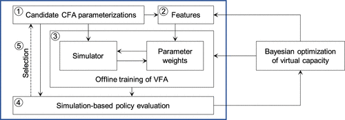
We begin by developing an approach for the DPLDMP without overbooking, as defined by (9). Building on this foundation, we extend our framework with a mechanism to optimize the virtual capacity vector in (13). The entire solution framework is summarized in Figure 2.
4.1.1. Demand Control and Allocation.
Although toy instances with a handful of compartments and points in time can be solved to optimality (Section 5.1.1), the curses of dimensionality (Powell 2022) render the computation of in (9) intractable for realistic problem sizes. Although is manageable because , its counterpart corresponds to a multidimensional resource allocation decision space that grows combinatorially in its dimensions. Similarly, the multidimensional matrices in lead to prohibitively large state and outcome spaces for real-world applications.
To overcome these challenges, we need to develop a suitable solution approach. Apart from the two sources of uncertainty induced by request arrivals and parcel pickups, a key characteristic of the DPLDMP stems from the two types of strongly interrelated decisions arising at different points in time. Consequently, the solution framework must not only encompass tailored components to handle each decision type on its own, but also properly address their interdependencies.
Well-performing allocation decisions ensure that the locker’s limited capacity is utilized efficiently and simultaneously create favorable conditions for subsequent demand control. This requires anticipating allocation decisions for pending orders and predicting new orders resulting from future demand control.
As shown in (12), optimal demand control essentially trades off a request’s immediate reward with its opportunity cost. As a result, demand control should factor in allocation decisions because they influence the available capacity in the compartments, shape the decision space for future demand control, and affect the capacity consumption caused by accepting the request, which is all reflected in the opportunity cost.
To handle the interdependencies between the two decision types, we propose a hierarchical approach. More precisely, our solution framework comprises two components, one for demand control and one for allocation, with different levels of sophistication. Given that demand control determines which requests turn into orders, it presents itself as a more promising lever to improve overall performance. By comparison, allocation merely serves as a secondary decision. Intuitively speaking, it is harder to compensate bad demand control decisions with good allocation decisions than vice versa. Bearing this in mind, we consciously limit the computational effort of the allocation component in favor of an elaborate demand control component.
Drawing on the framework by Powell (2022), we design the individual components as follows: Allocation is characterized by its extensive decision space. In light of this, we employ CFA, yielding a parameterized optimization model. This allows us to efficiently search the decision space with standard solvers. If the provider accepts a request during demand control, it turns into an order and typically stays in the system for several days depending on its lead time and pickup time. To properly estimate the decision’s downstream impact, we apply a parametric VFA.
Harnessing this architecture, we devise the following procedure to obtain the CFA and VFA parameters.
The vast set of potential CFA parameterizations necessitates tuning. However, the performance of a specific CFA parameter configuration also depends on demand control, whose VFA parameter weights in turn hinge on how allocation decisions are made as a result of the CFA parameters. Consequently, we need to train the VFA for each CFA parameterization we want to examine, which is computationally expensive. At the same time, we must keep the computational burden of the core of our solution framework moderate to be able to extend it to overbooking. We achieve this by predefining a promising subset of candidate CFA parameterizations through domain knowledge, aiming to create favorable conditions for demand control.
We embed the allocation scheme of a given CFA parameter configuration into the VFA feature design, thereby incorporating the impact of allocation into demand control. This yields a vector of features .
To train the VFA, we learn the parameter weights for the features through offline simulation. The simulator requires a given CFA parameterization, which determines the simulated allocation decisions (and the feature design), as an input and returns a vector of trained weights .
A specific CFA parameterization together with the correspondingly trained VFA form a candidate policy, whose performance is evaluated through simulation.
Among the evaluated candidate policies, we choose the best-performing one as the final policy.
In summary, we take the interdependencies between the two decision types into account by contriving candidate CFA parameterizations that aim at facilitating future demand control and, conversely, by constructing the features and training the VFA for the allocation schemes induced by the CFA parameters.
4.1.2. Virtual Capacity.
A key challenge to solving (13) lies in the fact that the objective cannot be represented with an analytical function. To address and obtain a policy for a given virtual capacity vector, we adopt the method described in the previous section. Consequently, evaluating the objective value in (13) is quite costly in terms of computational effort because we first have to train the VFA and then determine the objective value with simulation. To efficiently guide the solution process, we use BO. On a high level, for each CFA parameterization, we conduct a predefined number of iterations with BO. In each iteration, BO suggests a new virtual capacity vector (Section 4.4), for which we train the VFA and evaluate the resulting policy. We execute this procedure for every candidate CFA parameterization and select the best policy and virtual capacity in the end.
4.2. Cost Function Approximation
CFA involves solving a parameterized optimization model where the objective or constraints are modified to induce decisions that perform well over time and under uncertainty. This entails two steps: first, designing the parameterization (Section 4.2.1), and second, determining the parameter values (Section 4.2.2).
4.2.1. Design of Parameterization.
As a starting point for modifying the immediate reward function of allocation decisions, we identify two favorable circumstances for subsequent demand control.
In general, larger compartments tend to be more valuable as they fit more parcel sizes and offer more flexibility. Although Property 2 in Section 3.3 proves that it is not optimal to always assign parcels to the smallest available compartment, this principle still holds in many cases.
Having a specific compartment available for multiple consecutive days increases the likelihood of incoming requests being feasible. In light of this, we aspire to allocate orders such that we conserve available capacity in the compartments across several days to facilitate the construction of feasible tentative plans.
Bearing these two considerations in mind, we introduce the concept of capacity windows. With this term, we refer to a stretch of available capacity in the tentative allocation plan. It is characterized by its length , that is, the number of allocation decisions (days) it spans across and the size of the compartment in which it arises. For a specific tentative allocation plan, we let denote the number of capacity windows in compartments of size with length . Capacity windows serve as the basis for our CFA design as they encapsulate both the notion of preserving capacity across multiple days as well as the relevance of the compartment size. We weight with a corresponding parameter and obtain the CFA objective:
To properly link to the allocation decision , we formalize the CFA decision space in Online Appendix C.
4.2.2. Parameter Selection.
After specifying the CFA design, we need to determine suitable values for . A key challenge is posed by the large space of potential parameterizations that grows combinatorially with the number of compartment sizes D and window lengths F. To tackle it, one would typically resort to methods from the realm of stochastic search (Powell 2022, chapter 11.12). However, these methods require evaluating each generated parameter configuration. In our case, this is computationally expensive as the CFA parameters are also embedded in the VFA feature design and part of the VFA training procedure. More specifically, we have to retrain the VFA whenever the CFA parameters are adapted and then measure the performance of the resulting policy through simulation. Consequently, evaluating a sizeable number of parameters is hardly tractable. Instead, we limit the number of candidate parameterizations a priori through domain knowledge, thereby sidestepping the issue of excessive computational effort for parameter tuning.
Essentially, capacity windows are characterized by their length and the compartment size . Accordingly, we propose two objectives, each geared toward maximizing the number of capacity windows in hierarchical order of one of these attributes. To cover both, we optimize the objectives in lexicographic order. For the specific parameterizations, we refer to Online Appendix C. We solve the resulting integer program (IP) with standard software, thereby handling the curse of dimensionality in the allocation decision space.
4.3. Value Function Approximation
If an oracle was to provide us the optimal value function , applying the decision criterion in (12) becomes trivial. Essentially, it boils down to trading off the request’s immediate reward with the opportunity cost. The opportunity cost captures the potential displacement of future customers: Each accepted request consumes capacity, which might force the provider to reject future requests.
The curses of dimensionality render the computation of intractable for realistic problem sizes, compelling us to rely on approximation. Instead of computing the value for each state individually, we learn a parametric VFA with a vector of weights to obtain value estimates . As an input, we devise a set of features to extract relevant information from the state variable in Section 4.3.1. Subsequently, Section 4.3.2 sheds light on the procedure to learn the parameter weights , complemented by a detailed description of our modified version of experience replay in Section 4.3.3.
4.3.1. Feature Design.
As a preliminary consideration, we first establish which values we seek to approximate given that the value function can be computed for predecision states , postdecision states or pairs of predecision states and decisions . The latter corresponds to the Q-values typically used in RL, where rewards are modeled as a random variable. By contrast, we want to exploit the fact that rewards are a deterministic function of and in the DPLDMP, which is not possible with Q-values. If we were to approximate the values for , we would have to compute the expectation in (11), which is not tractable due to the curse of dimensionality in the outcome space. To sidestep this, the best-suited choice is to approximate the values of the postdecision states .
In a next step, we require an adequate representation of the information contained in in the form of a vector of features . In theory, one could directly use itself. However, this comes at the disadvantage of a relatively large number of features ( in total) and hence parameters to learn while foregoing the opportunity to incorporate domain knowledge. Specifically, offers no immediate insight into the implicit resource allocation task at the end of each day and the allocation logic induced by the CFA.
Intuitively speaking, the expected future rewards and thus the value of a state hinge on the available capacity and the incoming future demand, which are both uncertain. As an underlying strategy, we aim to capture an estimate of the available capacity through our features and then evaluate what can be achieved with it in terms of expected future rewards through the parameter weights . This general idea has proven successful in other domains, such as dynamic vehicle routing (Ulmer, Mattfeld, and Köster 2018) or integrated demand management and vehicle routing problems (Koch and Klein 2020).
To measure available capacity, we revert to the concept of capacity windows introduced in Section 4.2.1. For the CFA, capacity windows are determined based on the allocation decision space, which assumes that all customers use the maximum storage time. For the VFA features, we slightly adapt this to get an estimate of available capacity that also reflects the uncertain pickup behavior of customers. More specifically, we generate a total of U scenarios with sampled pickups for all pending orders and orders currently in the locker . In the latter case, we exploit the dwell time h and current point in time to obtain conditional pickup probabilities. For each scenario , we construct a tentative allocation plan by solving the IP in Online Appendix D. Note that the tentative plan with sampled pickups covers a slightly longer planning horizon to fully include the pickup times of orders allocated in .
To incorporate the allocation scheme in the feature design, we use the CFA parameters as objective coefficients. Note that we do not aim to perfectly predict future allocation decisions; the main purpose is to get an estimate on available capacity with reasonable computational effort that allows a differentiated evaluation according to compartment size as well as connectedness across multiple days. Given that we need a tentative plan for each scenario and that U should be sufficiently large, we reduce the computational burden by constructing the tentative plans as if all pickup times were known upfront.
In each scenario u, we extract the number of capacity windows per compartment size and length from the tentative allocation plan. Averaging across all scenarios, we obtain as input features for the VFA. Regarding the functional form, we opt for a linear approximation architecture with parameter weights and a constant intercept . Note that including an intercept is not only strongly recommended in general (Kutner et al. 2004, chapter 4.4), but also necessary in our specific setting: Even if all features take on the value zero, meaning that we estimate to have no available capacity during the limited planning horizon of the tentative allocation plan, we still expect to generate rewards in the long run once the capacity becomes unoccupied again, which is captured by the intercept.
Letting denote the vector of features and the vector of parameter weights, we specify as follows:
On the surface, (15) bears a strong resemblance to (14). However, note that they differ in two critical ways.
Pickup times. For the CFA, is calculated assuming every customer makes use of the maximum storage time, whereas the VFA features result from averaging across multiple sample realizations of pickups. We refrain from incorporating sampled pickups in the CFA for two reasons: First, although we can compute each scenario separately for the VFA, we would have to jointly optimize the allocation decision over all scenarios for the CFA. Second, the worst-case scenario is highly relevant for demand control as it is the foundation for the feasibility check, which motivates gearing allocation decisions toward it.
Determination of parameters. The VFA parameter weights aim at approximating the value function of a policy and are the result of a simulation-based learning process that requires a CFA parameter configuration as an input (Sections 4.1 and 4.3.2). By contrast, the CFA parameters are the result of tuning (Section 4.2.2 and Powell 2022, p. 613). Note that we cannot simply use the trained weights in the CFA objective because they are always trained for a specific allocation scheme. If we change the CFA parameters, we must retrain (and adapt the objective for computing the tentative allocation plans for ).
4.3.2. General Training Procedure.
To train the VFA parameter weights , we combine different RL techniques in a simulation-based learning process that is executed offline. Our algorithmic procedure encompasses two types of updates: Upon each simulated demand control decision, we update the parameter weights incrementally based on temporal difference (TD) learning (Sutton and Barto 2018). At the end of selected days, we additionally perform a second type of update using experience replay (ER; Lin 1993).
(
Initialization:
1: for do
2: repeat
3:
4: sample exogenous information to obtain
5: if then
6: make -greedy demand control decision to obtain
7: perform TD update and add experience to
8: if then
9: remove oldest experience from
10: end if
11: end if
12: until
13: make allocation decision to obtain
14: if then
15: perform ER update
16: end if
17: end for
In the subsequent paragraphs, we delve into the algorithmic procedure outlined in Algorithm 1 (we provide a more detailed pseudocode in Online Appendix D). As a first step, we introduce the parameters: The simulation runs for a total of days, and we use n to refer to simulated decision epochs. For decision making, we employ an exploration scheme . The ER parameters specify the size of the replay memory and the size of the samples drawn from it as well as the start and frequency of ER updates. Lastly, we require a CFA parameterization as it shapes the VFA features and governs allocation decisions during the simulation. We initialize the algorithm by setting all parameter weights to zero. Furthermore, the algorithm starts with an empty replay memory and with an initial postdecision state .
During each simulated day, we generate the next decision epoch by sampling exogenous information and transitioning into a new predecision state . In case of a request arrival, we make an -greedy demand control decision; that is, we choose the decision that is deemed optimal according to our current parameter weights with probability and select a random decision out of with probability . This induces the algorithm to try decisions that are perceived suboptimal according to the current parameter weights to verify their evaluation and ensure sufficient exploration. After demand control, the system evolves into . Based on this transition, we compute the TD error to update . The data collected during decision epoch n are stored as an experience that encompasses the feature vector of the previous postdecision state , as well as the feature vector resulting from rejection of the current request . Moreover, if the request is feasible, we include the postdecision state features for acceptance and the reward . For an infeasible request, we set and . If the size of the replay memory exceeds , we delete the oldest experience.
The sequence of demand control decisions and TD updates carries on until the day concludes with the allocation decision in , which is shaped by the CFA parameterization . In addition, after the first days, we perform an ER-based update for every days. The threshold serves to ensure that a sufficient amount of experience has accumulated in the replay memory.
4.3.3. Experience Replay Update.
For the ER update, we generate a simple random sample without replacement from , denoted by . The sample contains (up to) previously encountered decision epochs (if , ), each associated with a stored experience . Based on this data, we compute a value estimate (Section 3.2.7) for each sampled experience (with as an estimate for the reward rate; Online Appendix D). These estimates serve as prediction targets in a ridge regression to obtain updated parameter weights.
Note that our version of ER differs from its standard implementation in RL in the following four ways.
Postdecision state values. Instead of Q-values, we approximate postdecision state values. This entails adaptations that make the ER updates less off-policy, that is, the difference between the behavior policy used to generate data and the target policy to be approximated is less pronounced (Mnih et al. 2015). More specifically, the update targets in our version of ER are more on-policy as we generate them by making the decision that is considered optimal according to our current parameter weights instead of replaying the decision that was made at the time of collecting the experience. The distribution of experiences in the replay memory depends on previous parameter weights and is hence off-policy.
Ridge regression. During the ER update, we perform ridge regression to hedge against multicollinearity issues. To illustrate, if the number of longer capacity windows reduces after a request acceptance, this is accompanied by simultaneous shifts in other features, that is, the number of shorter windows increasing. Multicollinearity does not generally inhibit the predictive capabilities of the regression as long as new observations lie in the region of previous data (Kutner et al. 2004). However, given that the region of frequently encountered states changes over the course of training, we cannot guarantee that this prerequisite holds.
Two types of updates. Our approach of regular TD and periodic ER updates extends the Combined-Q algorithm by Zhang and Sutton (2017) that uses a combination of TD and ER updates in every decision epoch. Our reasoning for less frequent ER updates is as follows: The TD update is based on a single, brand new observation, that is, the data of the current decision epoch. As a complement, ER draws on a batch of previously stored experiences and keeps the value estimates in check for a larger sample of the state space, thereby increasing data efficiency and stabilizing the learning process (Mnih et al. 2015). However, focusing too much on ER runs the risk of fitting the value function to a large portion of states visited under previous policies that are in fact not relevant for the optimal policy. In VFA, we cannot hope to approximate every state value perfectly. Consequently, we mainly base the learning process on “fresh” data through TD updates and merely support it with less frequent ER updates.
Enforcing structure. Additionally, the ER update can be used to enforce structural properties in the value function by imposing constraints on the parameter weights (Section 5 and Online Appendix E).
4.4. Bayesian Optimization
The basic idea behind BO works as follows: We begin with a set of initial beliefs about the parameters to be optimized in the form of prior probability distributions. Sampling from these distributions, we generate data points, each consisting of a parameter configuration and the associated objective value. With these data, we update our beliefs, identify a promising new parameter candidate, and repeat the process. Consequently, BO amounts to a sequential search guided by the collected data instead of exhaustively searching a very limited space in a grid search or proceeding in a random search completely uninformed by previous data.
Although BO encompasses a variety of methods, we adopt the algorithm proposed by Bergstra et al. (2011). For the initial beliefs, we assume a uniform distribution over for and randomly initialize our data set. To evaluate a given virtual capacity vector, we derive the corresponding policy by training the VFA, incorporating the virtual capacity in the features and in the simulator. We apply the policy to multiple randomly sampled, finite customers streams and compute the average objective as an approximation of the true objective value in (13). Each subsequent iteration consists of two steps: First, the data set is partitioned into two groups based on a quantile threshold for the objective value. Using Kernel density estimation, we construct a surrogate model with two probability densities representing the better and worse groups of parameters, respectively. Second, the next parameter configuration is identified with an acquisition function that maximizes the ratio of the two densities to find a parameterization with a high probability of belonging to the better and low probability for the worse group. This new candidate is evaluated and added to the data set. We perform BO for a given number of iterations and select the best-performing virtual capacity.
5. Computational Study
In the following, we present our computational study. After explaining its setup in Section 5.1, the subsequent analysis serves four purposes: First, we assess the performance of our solution framework (Section 5.2). Second, we gain structural insights into the optimal policy by solving small problem instances to optimality (Section 5.3). Third, inspired by practice, we investigate the impact of heterogeneous pickup behavior (Section 5.4). Fourth, we explore the inherent tradeoff in overbooking (Section 5.5).
5.1. Design
In this section, we report all instance parameters (Sections 5.1.1 and 5.1.2), present the investigated policies (Section 5.1.3), and define the metrics (Sections 5.1.4) and bounds (Section 5.1.5) used for evaluation.
5.1.1. Small Instances.
Solving the DPLDMP to optimality is only tractable if the instances are restricted to a modest size. We propose the following setup with up to |S| = 878,541 predecision states.
Resources. We consider two compartment sizes and all configurations with and , resulting in a total of 15 distinct locker layouts. For readability, we encode the compartment sizes as S, M for and denote the locker layouts with a slight abuse of notation as .
Time. Because the instances differ regarding the locker capacity, we also vary the number of points in time T accordingly to adjust the expected number of request arrivals per day: .
Requests. We focus on a single customer type with an arrival probability of one at each point in time t. The lead time e equals one, two, or three days with equal probability of . The probabilities for the parcel sizes are proportional to the number of compartments per size, that is, .
Parcel pickups. The maximum storage time is days with a uniform pickup probability distribution.
Objective. We select for the failed delivery penalty; that is, there is no overbooking.
5.1.2. Large Instances.
Our analysis for the large instances is divided into two parts. In each part, the instances are further grouped into settings. The first part is strongly inspired by the Amazon case (Sethuraman et al. 2024). More specifically, it highlights how differences in the pickup speed of customer types affect the system. To simplify the analysis, we do not incorporate overbooking in this part yet, that is, . This also enables us to focus on the workings of the inner core of our solution concept because the optimal virtual capacity is known. The second part delves into overbooking and elucidates the tradeoff between rejected requests and failed deliveries. In a sensitivity analysis, we vary the pickup behavior of the entire customer population to assess how different levels of scarcity relate to the value of overbooking.
Having laid out the general structure, we first specify the parameters that apply to all settings.
Resources. We include three compartment sizes with , , and . Analogous to the small instances, we encode the compartment sizes as S, M, and L for , respectively.
Time. Ensuring a suitable level of scarcity relative to the locker capacity and given the tradeoff between temporal resolution and associated computational effort, each day consists of discrete points in time with the allocation decision in .
Requests. There are two customer types . At each point in time t, a customer of type arrives with probability 0.3, of type with probability 0.6, and with probability 0.1, there is no customer arrival. We consider to be premium customers with expedited shipping, leading to a lead time of with probability 1. For standard customers (), the lead time e equals one, two, three, four, or five days with a respective probability of 0.2, 0.2, 0.3, 0.2, and 0.1. The probabilities for the parcel sizes are identical for both customer types and are proportional to the number of compartments per size (, , for S, M, L).
Parcel pickups. The maximum storage time is days. Remember that we express the pickup time as a tuple where b represents the number of days after allocation and q the point in time (Section 3.1). We assume a uniform distribution for q, leading to a probability of for each point in time .
The individual settings differ with regard to the customer pickup behavior (more precisely, the probabilities for b) and the failed delivery penalty m. We state the probability distributions for b along with the expected value and standard deviation in Table 2. Note that represents how many days customers block a compartment on average and correlates with the scarcity of capacity while quantifies the level of uncertainty for pickups. The settings are structured as follows.
|
Table 2. Pickup Probability Distributions
| c | Number of days after allocation b | |||||
|---|---|---|---|---|---|---|
| 1 | 2 | 3 | ||||
| id | 1, 2 | 0.60 | 0.20 | 0.20 | 1.60 | 0.80 |
| pf | 1 | 0.80 | 0.10 | 0.10 | 1.30 | 0.64 |
| 2 | 0.50 | 0.25 | 0.25 | 1.75 | 0.83 | |
| pu | 1 | 0.94 | 0.04 | 0.02 | 1.08 | 0.34 |
| 2 | 0.43 | 0.28 | 0.29 | 1.86 | 0.84 | |
| idf | 1, 2 | 0.94 | 0.04 | 0.02 | 1.08 | 0.34 |
| ids | 1, 2 | 0.02 | 0.04 | 0.94 | 2.92 | 0.34 |
In the first part, centering around customer heterogeneity, we set the failed delivery penalty to and examine three pickup probability distributions, yielding three settings: With the first one, premium and standard customers exhibit the same behavior (id for identical). Under the second one, premium customers collect their parcels faster (pf for premium fast). Lastly, with the third distribution, we make this difference in pickup speed even more pronounced (pu for premium ultrafast). We select the probabilities for id based on the fact that about 60% of parcels are picked up within one day after delivery in practice (Hovi et al. 2023). For pf and pu, we specify the probabilities such that the aggregated distribution over the entire customer population remains unchanged; that is, in each setting, 60% of all parcels are picked up within one day, 20% on the second day, and 20% on the third day.
In the second part, we reconsider distribution id along with two additional distributions that represent extremely fast and slow pickups with high certainty (idf for identical fast and ids for identical slow). To keep our analysis concise, the distributions are kept identical for both customer types. A combination of one of the distributions id, ids, and idf with a penalty constitutes a setting in this part.
5.1.3. Policies.
Because of the two types of decisions present in the DPLDMP, each of the policies consists of two components. For the allocation component, we test three CFA parameterizations.
DL (first dimension, then length) is based on the concept of capacity windows (Section 4.2) and uses compartment size as the primary and window length as the secondary objective.
LD (first length, then dimension) only differs from DL in the lexicographic order of the objectives; that is, window length serves as the primary and compartment size as the secondary objective.
BU (bottom-up) acts as a benchmark that does not rely on capacity windows and instead focuses fully on the next allocation decision. It prioritizes using smaller compartments first (details in Online Appendix E).
For demand control, we compare our method to a practice-inspired and a myopic benchmark.
V-ER (experience replay) is our proposed solution approach from Section 4.3.
DLP (deterministic linear program) is an established method (Section 2) and similarly applied in practice (Sethuraman et al. 2024). We adapt this concept to the DPLDMP (details in Online Appendix E).
FC (feasibility control) is a purely myopic approach that accepts every feasible request.
To assess the contribution of certain algorithmic modules of V-ER, we generate two additional VFA variations by adapting or removing the corresponding parts in Algorithm 1 in the style of an ablation study.
V-CER (constrained experience replay) imposes constraints on the ridge regression for ER that enforce structural properties of the value function (Online Appendix D).
V-TD (temporal difference) only uses TD updates; that is, we eliminate line 15 in Algorithm 1.
We test all combinations of the approaches listed above, resulting in policies. We refer to the policies by with the demand control abbreviation in superscript and allocation in subscript, for example, .
To determine the virtual capacity , we perform 50 iterations of Bayesian optimization (after generating 10 random samples for initialization) in each setting with failed delivery penalty . For , it is straightforward to derive the optimal virtual capacity: In case of , we accept all incoming requests, that is, , and with , we prohibit overbooking, that is, . Note that in the former case, we set the virtual capacity to a sufficiently large number in the simulations as the allocation decisions are based on IPs that would otherwise become unbounded.
For the small instances, we compute the optimal policy with relative value iteration (Puterman 1994). We implemented all algorithms in Python 3.8 and solved the IPs for the feasibility check, CFA, and VFA features as well as the quadratic program for ER with Gurobi 10.0.3. For BO, we used the package hyperopt (Bergstra, Yamins, and Cox 2013). The experiments were conducted on a server with two Intel Xeon E7-8890 v3 processors (2.5 GHz, 18 cores) and 512 GB RAM. On average, the feasibility check took 0.01 seconds and the allocation decision 0.03 seconds. For demand control, decision times range from instantaneous (FC) to up to 0.7 seconds (V-ER). Details on hyperparameters are provided in Online Appendix F.
5.1.4. Metrics.
We use eight metrics to derive managerial insights into the policies’ control behavior.
The first three metrics categorize demand control decisions. Each metric represents a rate, calculated as the number of requests (with a specific combination of attributes, i.e., customer type, lead time, or parcel size) that received a given type of decision divided by the total number of requests (with those attributes).
The acceptance rate (AC) refers to the percentage of accepted requests.
The feasibility rejection rate (FR) captures requests rejected because of the feasibility check.
The anticipatory rejection rate (AR) corresponds to requests that are rejected despite being feasible.
The next three metrics characterize allocation decisions based on the proportion of orders (with certain attributes) that were allocated in a specific way out of the total number of orders (with the same attributes).
The exact fit rate (EF) reflects orders that are allocated to a compartment equal to the parcel size.
The feasibility upgrade rate (FU) indicates the percentage of orders upgraded to a larger compartment to maintain feasibility. It is derived by determining the number of upgrades that would result from BU (Section 5.1.3) because this approach only upgrades if strictly necessary.
The anticipatory upgrade rate (AU) covers the upgrades performed beyond those for feasibility.
In case of overbooking, we further refine the AC by jointly considering demand control and allocation.
The successful delivery rate (SD) regards the accepted requests successfully delivered to the locker.
The failed delivery rate (FD) concerns the accepted requests where the locker delivery failed.
Throughout the study, we report all metrics in percent. Note that AC, FR, AR and EF, FU, AU always sum to 100%, respectively, and that . In case of no overbooking, and .
We evaluate the metrics based on the entire state space for the small instances. In case of the realistically sized settings, we estimate the metrics with 30 randomly generated instances. For the sake of comparability, we consistently use the same 30 streams of customer arrivals in each setting. Consequently, the settings exclusively differ in the pickup behavior (due to the different pickup probability distributions in Table 2) and not in the sequence of incoming requests. The policies start with an empty locker and no pending orders and complete a warm-up phase of 75 days that are discarded to eliminate temporary effects caused by the initial state. We calculate the metrics per stream (consisting of 100 days after the warm-up) and compute the average per setting. For aggregate results, we subsequently average over all settings. We include the standard deviation across the instances for metrics reported per setting. To ensure that our study is representative of the system’s steady state, we tested different simulation horizons and verified that our results remain stable.
5.1.5. Optimality Gap and Upper Bound.
To assess performance, we use two instruments. Firstly, we compute the relative gap to the optimal policy based on 30 small instances covering 100 days and a prior warm-up phase of 75 days in Section 5.2. Instances with the same total number of compartments only differ in the parcel sizes as the distribution depends on the locker layout. Secondly, we provide upper bounds on the successful delivery rate in Section 5.5 using a full-information benchmark (Online Appendix E).
5.2. Solution Quality
In settings without overbooking, we can gauge the policies’ overall solution quality exclusively based on the AC. In the subsequent sections, we delve into our main findings.
5.2.1. Performance Assessment.
Figure 3 depicts the optimality gaps of the demand control approaches FC, DLP, and V-ER relative to the optimal policy across various locker layouts (in combination with the best allocation approach for each layout). The lookahead-based DLP strictly dominates myopic FC, and our method V-ER outperforms FC for the vast majority of layouts (the only exception being ). Interestingly, the DLP exhibits excellent performance for configurations with up to three compartments but loses its edge over V-ER with growing locker capacity, hinting at limited scalability. For layouts with a total of five or more compartments, V-ER consistently achieves the lowest gaps.
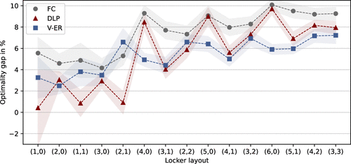
Note. Ordered by locker capacity and compartment size, with 99% confidence intervals.
To evaluate performance in the large instances without overbooking, we report the average improvement compared with the best-performing myopic approach in Figure 4 together with the 99% confidence intervals. Overall, the results support our hypothesis that demand control is the stronger lever for improvement. We identify as the best policy with a statistically significant average improvement of 3.4%.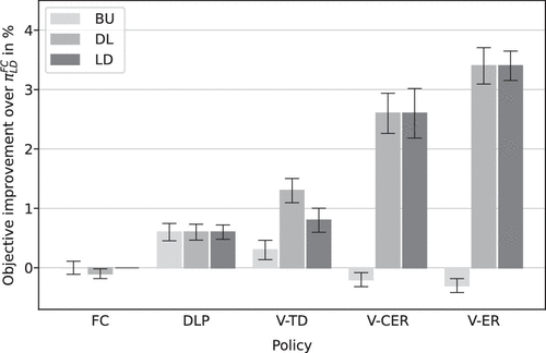
Note. With 99% confidence intervals.
Note that from a practical viewpoint, even seemingly modest gains in the acceptance rate are meaningful.
Projected to one year, accepts 4,959 requests on average per setting compared with 4,795 by . Although our study focuses on a single locker, our approach can be deployed across entire networks with substantial throughput in absolute terms. To illustrate, InPost operates more than 10,000 lockers in the United Kingdom, where lockers processed 87 million deliveries in 2024 (Retail Economics and InPost 2025).
The costs of acceptance and rejection are highly asymmetric. On the one hand, an additional locker delivery entails negligible operational costs. On the other hand, besides causing dissatisfaction, rejections may result in the customer selecting a more costly option such as home delivery or entirely abandoning the purchase. According to a survey, 48% of online shoppers frequently abandon their baskets because of delivery options (DHL 2024). In summary, each additionally served customer spares the provider from the potentially severe ramifications of rejecting a request at basically no cost (the only negative effect of an acceptance decision being the potential displacement of future requests).
5.2.2. VFA Variants.
Regarding the tested VFA variants, Figure 4 shows that if we solely rely on TD updates (V-TD), the policies struggle to outperform the benchmarks. For capacity window–based allocation (DL and LD), the approaches with ER (V-CER and V-ER) lead to substantial performance improvements. Enforcing structure in the value function (V-CER) generated further improvements in pretests with additional customer priority weights. However, for the considered settings, we declare as the best policy.
To explain the superior performance with ER, recall that the VFA features are calculated based on sample realizations of pickups. This introduces randomness into the mapping of postdecision states to features. ER updates help to alleviate any destabilizing effects that might arise from our feature design. Remarkably, this observation does not hold for BU. To get to the bottom of this, we highlight two key differences. Firstly, DL and LD involve lexicographic optimization, reducing the likelihood of a nonunique tentative allocation plan. By contrast, there might regularly exist multiple plans for BU, adding a second source of randomness to the state feature mapping. Secondly, DL and LD are more well aligned with the VFA features because they are based on capacity windows. Our findings indicate that the solution framework must take into account interdependencies between decision types. This holds in both directions: Allocation must match demand control (VFA performs better when combined with DL or LD) and vice versa, demand control must match allocation. To illustrate this, we performed pretests with differing objectives for the VFA features and allocation. The results showed that performance deteriorates drastically; that is, the VFA cannot handle strongly differing objectives for feature calculation and allocation even if trained on it.
5.3. Characterization of the Optimal Policy
To gain a better understanding of the optimal policy’s decision making across different regions of the state space, we take a closer look at for locker layout . For this purpose, we introduce an aggregate representation of the predecision states. More precisely, we use the number of orders currently in the system per (compartment) size to represent a predecision state with for all . This allows us to group states according to their aggregate representation. Inspired by Fleckenstein et al. (2025), we compute the metrics per group and display them in heat maps.
Figure 5 depicts the demand control metrics for different request types. Each metric entails six plots where the rows correspond to the parcel size and the columns to the lead time of the newly arrived request, for which we analyze the demand control decision. Because we consider two compartment sizes, the states are represented by and , resulting in two-dimensional heat maps. Analogously, Figure 6 illustrates the allocation metrics. Our analysis is organized into four parts, which we present in the following.
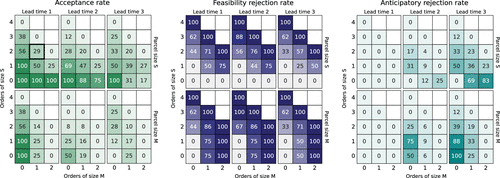
Note. Highlighted example: The acceptance rate of the optimal policy for a request with a parcel of size S and a lead time of one day in predecision states with orders of size S and orders of size M in the system equals 29%.
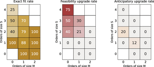
5.3.1. Lead Time.
A column-wise comparison of the plots shows that the AC tends to be highest for a lead time of day. Additionally, the AC of small parcels with exceeds its counterpart for in the majority of cases. Simultaneously, the FR is lowest for because most of the demand for the desired delivery date is yet to come at the time of the request’s arrival. By contrast, exhibits a high FR because of compatibility issues: Because of the maximum storage time , requests with cannot be assigned to the same compartment as orders with remaining fulfillment time or in the tentative allocation plan. For medium-sized parcels, this is exacerbated by the lack of upgrading possibilities. Filling the gap between AC and FR, the AR peaks for and declines with a decreasing lead time, equaling 0% for all states at lead time . We trace our findings back to two reasons: Firstly, by preferring a short lead time of , the optimal policy avoids committing to orders early (especially with larger parcels since they are eligible for fewer compartments). Secondly, orders with high lead times remain longer in the system and may thereby impact the feasibility check of many subsequent requests, rendering them less desirable.
5.3.2. Parcel Size.
Comparing the first and second row of plots, we find that the AC of the optimal policy declines with increasing parcel size. We attribute this phenomenon to two causes. Firstly, requests with larger parcels are less likely to be feasible because of a lower number of compatible compartments, resulting in a higher FR. Secondly, as shown in Property 1, a request’s opportunity cost rises monotonically with its parcel size. Higher opportunity costs reduce the chances that Inequality (12) holds, thereby leading to an anticipatory rejection. Note that the AR of size M parcels does not necessarily exceed the one for small parcels throughout the entire state space due to the already high FR of the former.
5.3.3. System Load.
In general, the AC tends to increase with a decreasing number of orders in the system, that is, toward the bottom left corner of the plots, because capacity is less scarce in these regions of the state space. However, there are notable exceptions for lead time , especially in combination with a medium-sized parcel: If there are no orders in the system, the AC equals . By contrast, if the number of existing orders grows, the AC also tends to become larger, which might appear counterintuitive at first glance. The rationale behind this pattern goes as follows: A completely empty system represents ideal conditions where the policy is comparatively picky about which requests it accepts, yielding a high AR for size M parcels with . In a less desirable state with a higher system load, the policy becomes more inclined to accept generally unfavorable requests. More specifically, existing orders can create gaps in the tentative allocation plan (similar to the observations in Property 2) such that an otherwise undesirable request fits well, making it more attractive.
5.3.4. Upgrades.
As expected, Figure 6 shows that upgrades only occur if the number of upgradeable orders is sufficiently high. In case of a substantial amount of small orders, upgrading becomes necessary to maintain feasibility. The optimal policy performs anticipatory upgrades in two specific predecision states. The first one resembles the example from Property 2. The second state involves an empty locker, a small pending order with , and one small order to be allocated. The optimal policy upgrades the latter to the medium-sized compartment such that the small one is guaranteed to be available in the next allocation decision. Otherwise, it might be forced to grant a feasibility upgrade in the subsequent allocation decision, which would potentially block the more valuable medium-sized compartment until a later point in time.
5.4. Policy Characterization Under Heterogeneous Pickup Behavior
Mirroring the previous section, we characterize the decision making of our approach as well as the benchmarks and to investigate the impact of differences in pickup speed between customer types.
5.4.1. Setting.
Table 3 presents the demand control metrics of the investigated policies per setting (with the standard deviations in brackets). In line with our findings from Section 5.2, consistently achieves the highest AC. The improvement over and is statistically significant at the 1% significance level and ranges between 2.2% and 3.9%. Its extent clearly depends on the setting: If the customer types are identical (id), individual requests merely differ in the parcel size and lead time, such that the displacement effects and hence the demand management potential are comparatively low. The more pronounced the difference in how valuable customer types are due to their pickup behavior, the more worthwhile our approach becomes.
|
Table 3. Demand Control Metrics
| id | pf | pu | ||
|---|---|---|---|---|
| AC | 73.4 (1.0) | 73.0 (1.1) | 72.7 (1.1) | |
| FR | 26.6 (1.0) | 27.0 (1.1) | 27.3 (1.1) | |
| AR | 0.0 (0.0) | 0.0 (0.0) | 0.0 (0.0) | |
| AC | 73.7 (1.0) | 73.4 (1.0) | 73.3 (1.1) | |
| FR | 25.7 (1.0) | 25.9 (1.0) | 25.8 (1.1) | |
| AR | 0.6 (0.2) | 0.7 (0.3) | 0.9 (0.3) | |
| AC | 75.3 (1.0) | 75.8 (0.9) | 75.5 (0.8) | |
| FR | 17.8 (1.4) | 16.7 (1.4) | 12.7 (1.5) | |
| AR | 6.9 (0.9) | 7.5 (0.9) | 11.8 (1.2) |
By design, always leads to an AR of 0%. Similarly, exhibits a low AR, which we explain as follows: The DLP largely ignores the effects of stochastic information realizing over time. Crucially, it neglects the impact of the feasibility check and consequently suffers from a systematic underestimation of opportunity cost. In comparison, our policy can capture the downstream impact of a decision in the DPLDMP more accurately and makes by far the most use of anticipatory rejections, yielding a substantially more active steering of demand. The aggressiveness of its control behavior intensifies from id to pu.
5.4.2. Customer Type.
To further shed light on the policies, we report the demand control metrics per customer type and setting in Table 4. Because equals a first-come-first-served policy, its AC for standard customers is considerably higher than for premium customers, who arrive on short notice and consequently experience an elevated FR. Furthermore, the AC of standard customers remains stable across the three pickup distributions. The declining pickup speed of this customer type reduces the available capacity and increases the chances for infeasibility, resulting in a growing FR for premium customers.
|
Table 4. Demand Control Metrics per Customer Type
| id | pf | pu | |||||
|---|---|---|---|---|---|---|---|
| Premium | Standard | Premium | Standard | Premium | Standard | ||
| AC | 59.9 | 80.1 | 59.0 | 80.0 | 58.8 | 79.8 | |
| FR | 40.1 | 19.9 | 41.0 | 20.0 | 41.2 | 20.2 | |
| AR | 0.0 | 0.0 | 0.0 | 0.0 | 0.0 | 0.0 | |
| AC | 61.2 | 80.0 | 60.1 | 80.0 | 60.6 | 79.7 | |
| FR | 38.8 | 19.2 | 39.9 | 18.9 | 39.4 | 19.0 | |
| AR | 0.0 | 0.8 | 0.0 | 1.1 | 0.0 | 1.3 | |
| AC | 69.2 | 78.3 | 72.6 | 77.4 | 79.5 | 73.5 | |
| FR | 27.9 | 12.8 | 26.5 | 11.7 | 20.0 | 8.9 | |
| AR | 2.9 | 8.9 | 0.9 | 10.9 | 0.5 | 17.6 | |
By contrast, actively reserves capacity for premium customers, leading to a generally higher AC for these customers than the other policies. Comparing the three policies, we observe that generates a substantial rise in the AC for premium customers, whereas the decline for standard customers is relatively moderate. If the premium customers become more attractive due to their pickup behavior, the balance shifts increasingly in favor of them due to a boost in the AR for standard customers and a simultaneous decline in the AR for premium customers. The AR of follows a similar pattern as , but much less pronounced. As a result, its metrics barely differ from those of . Table 3 demonstrates that is the only policy that benefits from exploiting the quicker pickup speed of premium customers in pf and pu.
5.4.3. Lead Time.
Digging deeper, we next analyze the impact of the lead time e for standard customers in Table 5. The first-come-first-served nature of becomes evident with an AC of about 100% for longer lead times that sharply declines for due to a rising FR. By contrast, reduces the AC for longer lead times and instead favors requests with , mimicking the optimal policy (Section 5.3.1). More precisely, aims to maintain flexibility by not committing too early to standard customers and instead reserves capacity for premium customers. However, reserving capacity for premium customers too aggressively means foregoing rewards from accepting standard customers. Consequently, the policy fills up remaining capacity with standard customers once it gets more information on the arrival of premium customers. From id to pu, the ACs of shrink because the decreased pickup speed erodes the appeal of accepting standard customers. In principle, also replicates the tendency of toward short lead times but again performs anticipatory rejections only sparingly.
|
Table 5. Demand Control Metrics per Lead Time
| id | pf | pu | ||||||||||||||
|---|---|---|---|---|---|---|---|---|---|---|---|---|---|---|---|---|
| Standard | Standard | Standard | ||||||||||||||
| 1 | 2 | 3 | 4 | 5 | 1 | 2 | 3 | 4 | 5 | 1 | 2 | 3 | 4 | 5 | ||
| AC | 60.1 | 63.5 | 85.0 | 99.0 | 100 | 59.8 | 62.8 | 85.3 | 98.9 | 99.9 | 58.7 | 62.5 | 85.3 | 98.9 | 99.9 | |
| FR | 39.9 | 36.5 | 15.0 | 1.0 | 0.0 | 40.2 | 37.2 | 14.7 | 1.1 | 0.1 | 41.3 | 37.5 | 14.7 | 1.1 | 0.1 | |
| AR | 0.0 | 0.0 | 0.0 | 0.0 | 0.0 | 0.0 | 0.0 | 0.0 | 0.0 | 0.0 | 0.0 | 0.0 | 0.0 | 0.0 | 0.0 | |
| AC | 60.6 | 64.6 | 85.0 | 97.2 | 98.9 | 61.1 | 64.2 | 85.2 | 96.9 | 99.0 | 60.5 | 63.8 | 85.1 | 96.4 | 99.0 | |
| FR | 39.4 | 35.3 | 14.0 | 0.8 | 0.0 | 38.9 | 35.7 | 13.3 | 0.6 | 0.1 | 39.5 | 36.1 | 13.1 | 0.6 | 0.0 | |
| AR | 0.0 | 0.1 | 1.0 | 2.0 | 1.1 | 0.0 | 0.1 | 1.5 | 2.5 | 0.9 | 0.0 | 0.1 | 1.8 | 3.0 | 1.0 | |
| AC | 69.8 | 65.7 | 78.5 | 92.4 | 91.5 | 68.7 | 66.2 | 78.8 | 89.4 | 88.1 | 65.0 | 55.0 | 75.7 | 90.0 | 87.3 | |
| FR | 27.2 | 24.7 | 8.0 | 0.1 | 0.0 | 25.6 | 23.3 | 6.8 | 0.0 | 0.0 | 19.7 | 17.0 | 5.5 | 0.0 | 0.0 | |
| AR | 3.0 | 9.6 | 13.5 | 7.5 | 8.5 | 5.7 | 10.5 | 14.4 | 10.6 | 11.9 | 15.3 | 28.0 | 18.8 | 10.0 | 12.7 | |
5.4.4. Parcel Size.
In Table 6, we investigate the demand control metrics per customer type and parcel size. For all policies, the AC drops with increasing parcel size. This is to be expected given that larger parcels fit less compartments, leading to an increased FR. Matching our previous findings, and produce lower ACs for premium than for standard customers across all parcel sizes. By comparison, drastically raises the AC for premium customers, especially for medium- and large-sized parcels, with the intensity again depending on how attractive premium customers are compared with standard customers. Clearly, the policy is able to trade off the higher opportunity cost of larger parcels (Property 1) with the pickup speed of the customer type and hence distinguishes between standard and premium customers. Remarkably, the AC for small parcels of standard customers under is higher than for the other policies. This shows that maintains flexibility not only through controlling lead times, but also by favoring small parcels from standard customers. Overall, Table 6 illustrates that standard customers with large parcels mainly “pay the price” for the superior performance of in the form of a substantially reduced AC. As before, shows a similar structure in its AR but rejects feasible requests only reluctantly.
|
Table 6. Demand Control Metrics per Parcel Size
| id | pf | pu | |||||||||||||||||
|---|---|---|---|---|---|---|---|---|---|---|---|---|---|---|---|---|---|---|---|
| Premium | Standard | Premium | Standard | Premium | Standard | ||||||||||||||
| S | M | L | S | M | L | S | M | L | S | M | L | S | M | L | S | M | L | ||
| AC | 73.6 | 53.8 | 31.6 | 88.2 | 77.6 | 61.4 | 72.5 | 53.0 | 30.8 | 88.2 | 77.6 | 60.6 | 72.3 | 52.7 | 30.6 | 87.9 | 77.5 | 60.3 | |
| FR | 26.4 | 46.2 | 68.4 | 11.8 | 22.4 | 38.6 | 27.5 | 47.0 | 69.2 | 11.8 | 22.4 | 39.4 | 27.7 | 47.3 | 69.4 | 12.1 | 22.5 | 39.7 | |
| AR | 0.0 | 0.0 | 0.0 | 0.0 | 0.0 | 0.0 | 0.0 | 0.0 | 0.0 | 0.0 | 0.0 | 0.0 | 0.0 | 0.0 | 0.0 | 0.0 | 0.0 | 0.0 | |
| AC | 74.6 | 54.8 | 33.6 | 88.1 | 77.7 | 60.5 | 73.6 | 54.2 | 31.9 | 88.1 | 77.9 | 60.4 | 73.9 | 54.7 | 32.9 | 88.0 | 77.1 | 60.3 | |
| FR | 25.4 | 45.2 | 66.4 | 11.4 | 21.5 | 37.5 | 26.4 | 45.8 | 68.1 | 11.4 | 21.1 | 36.7 | 26.1 | 45.3 | 67.1 | 11.4 | 21.6 | 36.4 | |
| AR | 0.0 | 0.0 | 0.0 | 0.5 | 0.8 | 2.0 | 0.0 | 0.0 | 0.0 | 0.5 | 1.0 | 2.9 | 0.0 | 0.0 | 0.0 | 0.6 | 1.3 | 3.3 | |
| AC | 79.0 | 66.8 | 44.6 | 91.1 | 84.3 | 29.1 | 79.5 | 68.6 | 59.9 | 91.5 | 85.4 | 19.8 | 83.8 | 77.3 | 71.1 | 93.1 | 72.9 | 17.0 | |
| FR | 20.9 | 32.8 | 38.8 | 8.9 | 15.2 | 19.0 | 20.5 | 31.3 | 35.0 | 8.5 | 13.8 | 17.3 | 16.0 | 22.2 | 27.4 | 6.7 | 10.1 | 13.2 | |
| AR | 0.1 | 0.4 | 16.6 | 0.0 | 0.5 | 51.9 | 0.0 | 0.1 | 5.1 | 0.0 | 0.8 | 62.9 | 0.2 | 0.5 | 1.5 | 0.2 | 17.0 | 69.8 | |
5.4.5. System Load.
Inspired by Section 5.3.3, we examine the policies’ control behavior across regions of the predecision state space. Given that acts like a first-come-first-served policy and that follows a very passive approach to demand management, they display the superficially intuitive logic of a diminishing AC with an increasing number of orders in the system. Notably, our approach is the only of the three policies where some request characteristics, namely a lead time of four or more days, exhibit a perceptible pattern of the AC growing with the system load, analogous to the behavior of the optimal policy. To illustrate, we plot the AC of for standard requests with lead time in setting pf in Figure 7. We observe an increase in the AC especially with a rising number of size L orders in the system.
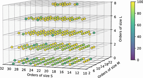
Note. For the sake of visual clarity, the number of orders per compartment size is aggregated in steps of two, and we only display areas with at least three corresponding states visited.
5.4.6. Upgrades.
In Table 7, we summarize the allocation metrics. Because each of the three policies performs its allocation decisions based on capacity windows, they all harness anticipatory upgrades to some degree with AU generally dominating FU. Drawing on our findings from the optimal policy in Section 5.3.4, we know that feasibility upgrades mostly occur in regions of the state space where the number of upgradeable orders is substantial. However, the metrics for the large instances only cover the parts of the state space that were actually visited during the simulated customer streams instead of its entirety. Consequently, rather extreme regions with a high FU may be underrepresented. Additionally, an inherently high AU may automatically contribute to a lower FU. Comparing the three policies, has a consistently higher propensity to perform upgrades. This matches our observations from Section 5.4.4: The policy favors small parcels and shuns large parcels of standard customers, which is amplified by differences in pickup speed. On a more granular level, Table 8 provides the allocation metrics per compartment size. Small compartments are only compatible with exactly fitting parcels, leading to an EF of 100%. Notably, only about half of the parcels allocated to large compartments under are in fact large. Anticipatory upgrades represent a sizable portion of these allocations, both in comparison with the other compartment sizes and policies.
|
Table 7. Allocation Metrics
| id | pf | pu | ||
|---|---|---|---|---|
| EF | 93.6 (1.1) | 93.5 (1.1) | 93.4 (1.2) | |
| FU | 1.2 (0.9) | 1.3 (0.9) | 1.4 (1.0) | |
| AU | 5.3 (0.4) | 5.2 (0.4) | 5.2 (0.3) | |
| EF | 93.3 (1.1) | 93.4 (1.1) | 93.3 (1.1) | |
| FU | 1.2 (0.9) | 1.3 (0.9) | 1.4 (0.9) | |
| AU | 5.4 (0.3) | 5.3 (0.3) | 5.3 (0.3) | |
| EF | 90.5 (1.2) | 89.7 (1.0) | 89.5 (1.2) | |
| FU | 2.2 (1.0) | 2.4 (0.8) | 2.7 (0.9) | |
| AU | 7.3 (0.4) | 7.8 (0.4) | 7.9 (0.4) |
|
Table 8. Allocation Metrics per Compartment Size
| id | pf | pu | ||||||||
|---|---|---|---|---|---|---|---|---|---|---|
| S | M | L | S | M | L | S | M | L | ||
| EF | 100.0 | 89.6 | 79.8 | 100.0 | 89.7 | 79.3 | 100.0 | 89.7 | 78.7 | |
| FU | 0.0 | 1.5 | 4.5 | 0.0 | 1.7 | 5.1 | 0.0 | 1.8 | 5.0 | |
| AU | 0.0 | 8.8 | 15.6 | 0.0 | 8.7 | 15.6 | 0.0 | 8.4 | 16.3 | |
| EF | 100.0 | 89.6 | 78.7 | 100.0 | 89.5 | 79.1 | 100.0 | 89.3 | 78.7 | |
| FU | 0.0 | 1.6 | 4.7 | 0.0 | 1.8 | 4.6 | 0.0 | 2.1 | 4.6 | |
| AU | 0.0 | 8.8 | 16.6 | 0.0 | 8.7 | 16.3 | 0.0 | 8.5 | 16.6 | |
| EF | 100.0 | 90.3 | 55.3 | 100.0 | 90.3 | 51.4 | 100.0 | 86.8 | 56.3 | |
| FU | 0.0 | 2.8 | 8.8 | 0.0 | 3.2 | 9.2 | 0.0 | 4.9 | 7.0 | |
| AU | 0.0 | 6.9 | 35.9 | 0.0 | 6.5 | 39.4 | 0.0 | 8.2 | 36.6 | |
5.5. Overbooking
To conclude our computational study, we extend our analysis to overbooking. First, we reconsider pickup distribution id and expand its results. Second, we examine the interplay with the scarcity of capacity.
5.5.1. Extension of Previous Results.
Judging the solution quality in the context of overbooking requires a more intricate investigation because of two conflicting objectives: One the one hand, the provider would like to maximize the successful delivery rate (SD), whereas, on the other hand, keeping the failed delivery rate (FD) as low as possible. Instead of a single optimal solution, there exists a Pareto front that the decision maker can explore by varying the failed delivery penalty m. We present our results for the best-performing policy setup, that is, V-ER in combination with a setting-dependent allocation approach, in Table 9. Apart from the metrics, we include the gap to the upper bound and the virtual capacity .
|
Table 9. Overbooking Metrics for Setting id
| Penalty | 0 | 2 | 3 | 4 | |
|---|---|---|---|---|---|
| AC | 100 (0.0) | 93.5 (0.8) | 90.2 (1.0) | 90.2 (1.0) | 73.3 (0.7) |
| SD | 91.3 (0.8) | 89.4 (0.9) | 87.6 (0.8) | 87.6 (0.8) | 73.3 (0.7) |
| FD | 8.7 (0.8) | 4.1 (0.5) | 2.6 (0.4) | 2.6 (0.4) | 0.0 (0.0) |
| Gap to | 2.5 (0.4) | 4.7 (0.5) | 6.9 (0.7) | 6.9 (0.7) | 23.7 (1.1) |
Column equals our results from the preceding section. The conservative choice of ensures that failed deliveries do not occur at all. However, this comes at quite a high price for SD, which is reflected in the noticeable gap to . On the opposite end of the spectrum, column represents the other extreme where the provider simply accepts every incoming request. This strategy generates a markedly higher SD with a strikingly lower gap to but comes at the cost of about 8.7% of deliveries failing. Varying m opens the door to a range of potential strategies for the provider. With , we observe a slight reduction of the SD compared with but can cut the FD in half. This development continues for and levels out for . Our approach of optimizing the virtual capacity for a given penalty enables the provider to close the gap to while simultaneously determining an acceptable level for FD. At the end of the day, this boils down to a managerial decision.
5.5.2. Impact of Scarcity.
To understand how different levels of scarcity influence the effectiveness of overbooking, we consider two rather extreme scenarios for the pickup probability distributions where all customers either collect their parcels very promptly (idf) or slowly (ids) with high certainty. Table 10 reveals that if the pickup speed is generally fast, overbooking allows the provider to serve nearly all requests successfully and achieve remarkably low gaps to the upper bound . Because capacity is less scarce, only a small fraction of deliveries fails. Nevertheless, optimizing the virtual capacity enables the provider to lower the FD by 37% for compared with , entailing only a tiny reduction in the SD. This illustrates the merit of our approach to optimize the virtual capacity for varying penalties. Under extremely slow pickups, there is no benefit to overbooking as the worst-case assumption is a quite accurate representation of actual customer behavior. The SD is drastically reduced compared with the other scenarios, illustrating that incentivizing customers to a prompt pickup is a promising lever to increase the throughput of the system.
|
Table 10. Metrics for Settings with Extreme Pickup Behavior
| idf | ids | |||||||||
|---|---|---|---|---|---|---|---|---|---|---|
| 0 | 2 | 3 | 4 | 0 | 2 | 3 | 4 | |||
| AC | 100 (0.0) | 99.6 (0.2) | 99.1 (0.4) | 99.1 (0.4) | 79.8 (1.0) | 100 (0.0) | 55.1 (0.5) | 55.1 (0.5) | 55.1 (0.5) | 55.1 (0.5) |
| SD | 98.9 (0.3) | 98.7 (0.3) | 98.4 (0.4) | 98.4 (0.4) | 79.8 (1.0) | 56.7 (0.5) | 55.1 (0.5) | 55.1 (0.5) | 55.1 (0.5) | 55.1 (0.5) |
| FD | 1.1 (0.3) | 0.9 (0.2) | 0.7 (0.2) | 0.7 (0.2) | 0.0 (0.0) | 43.3 (0.5) | 0.0 (0.0) | 0.0 (0.0) | 0.0 (0.0) | 0.0 (0.0) |
| Gap to | 0.0 (0.1) | 0.2 (0.1) | 0.5 (0.2) | 0.5 (0.2) | 24.0 (1.6) | 2.1 (0.7) | 5.1 (0.9) | 5.1 (0.9) | 5.1 (0.9) | 5.1 (0.9) |
6. Conclusion and Outlook
This paper introduces a novel problem to dynamically manage the demand for parcel lockers. Its distinguishing features are uncertain resource usage durations in combination with an “upgrading” mechanism due to different compartment sizes and a generalization to overbooking. We develop a solution framework that handles the interdependencies between two decision types arising at different points in time. As a general methodological contribution, we augment the VFA training process with a modified version of ER. In the style of an ablation study, we quantify the resulting performance contribution: Although pure temporal difference updates lead to a performance improvement of 1.3% compared with the myopic benchmark, incorporating ER yields an improvement of 3.4%.
The large throughput of real-world locker networks and a highly asymmetric cost structure of the demand control decision underline the practical significance of increased acceptance rates. From a managerial perspective, our results show that the performance gains of our policy increase with the heterogeneity of customer types. These improvements mainly result from reserving capacity for customers with a fast pickup speed and preserving flexibility by favoring small parcels and short lead times. However, we also show that certain requests (large parcels of customers with slow pickup speed) get rejected disproportionately often.
We demonstrate that fully preventing failed locker deliveries immensely affects the acceptance rate. With overbooking, the provider can strike a balance between rejected requests and failed deliveries. Our results indicate that a slight increase in failed deliveries already generates a substantial rise in the number of served customers. Conversely, our method of optimizing virtual capacity produces a notable reduction in failed deliveries at the expense of only slightly fewer served customers compared with simply accepting all requests.
Concluding our work, we identify several promising areas for future research:
Overbooking. Our work sheds light on an intricate tradeoff between rejected requests and failed deliveries. This necessitates a managerial decision where the acceptable degree of overbooking must be calibrated carefully, presenting an intriguing starting point for future work.
Fairness. Our results indicate that demand management may systematically disadvantage certain customer groups. To mitigate this, future work could investigate fairness measures, for example, by introducing weighting factors for larger parcels.
Planning levels. The insights gained from our operational perspective could be incorporated into strategic problems, such as location planning (Mancini, Gansterer, and Triki 2023).
Business models. Many questions pertaining to specific business models remain unexplored. For example, a mobile locker provider offering both home and locker delivery (Kötschau, Soeffker, and Ehmke 2023) should consider demand management and routing integratively.
The open access publication of this article was supported by the publication fund of the University of Augsburg.
References
- (2025) Learning dynamic selection and pricing of out-of-home deliveries. Transportation Sci. 59(2):250–278.Link, Google Scholar
Amazon (2023) How to use Amazon Locker, the free and convenient way to pick up packages securely outside of your home. Retrieved September 3, 2024, https://www.aboutamazon.com/news/operations/how-to-use-amazon-locker.Google Scholar- (2022) Technical note—Bifurcating constraints to improve approximation ratios for network revenue management with reusable resources. Oper. Res. 70(4):2226–2236.Link, Google Scholar
- (2013)
Making a science of model search: Hyperparameter optimization in hundreds of dimensions for vision architectures . Dasgupta S, McAllester D, eds. Proc. 30th Internat. Conf. Machine Learn., vol. 28 (PMLR, New York), 115–123.Google Scholar - (2011) Algorithms for hyper-parameter optimization. Shawe-Taylor J, Zemel R, Bartlett P, Pereira F, Weinberger K, eds. Advances in Neural Information Processing Systems, vol. 24 (Curran Associates, Red Hook, NY).Google Scholar
- (2021) Last-mile delivery concepts: A survey from an operational research perspective. OR Spectrum 43:1–58.Crossref, Google Scholar
DHL (2022) DHL online shopper report 2022. Retrieved September 3, 2024, https://www.dhl.com/content/dam/dhl/local/global/dhl-parcel/documents/pdf/g0-parcelconnect-dhl-online-shopper-report-2022-ebook.pdf.Google ScholarDHL (2024) 2024 e-commerce trends report. Retrieved February 19, 2026, https://www.dhl.com/content/dam/dhl/local/global/dhl-ecommerce/documents/pdf/g0-dhl-e-commerce-trends-report-2024.pdf.Google Scholar- (2021) A large neighborhood search approach to the vehicle routing problem with delivery options. Transportation Res. Part B: Methodological 144:103–132.Crossref, Google Scholar
- (2023) Recent advances in integrating demand management and vehicle routing: A methodological review. Eur. J. Oper. Res. 306(2):499–518.Crossref, Google Scholar
- (2025) Explaining the performance impact of opportunity costs approximation in integrated demand management and vehicle routing. EURO J. Transp. Logist. 14:100166.Google Scholar
- (2024) Demand steering in a last-mile delivery problem with home and pickup point delivery options. Transportation Sci. 58(2):454–473.Link, Google Scholar
- (2009) Upgrades, upsells and pricing in revenue management. Working paper, Columbia University, New York.Google Scholar
- (2019) Revenue Management and Pricing Analytics (Springer, New York).Crossref, Google Scholar
- (2022) Online assortment optimization with reusable resources. Management Sci. 68(7):4772–4785.Link, Google Scholar
- (2020) How much to tell your customer?: A survey of three perspectives on selling strategies with incompletely specified products. Eur. J. Oper. Res. 280(3):793–817.Crossref, Google Scholar
- (2015) On the incorporation of upgrades into airline network revenue management. Rev. Managerial Sci. 9:635–660.Crossref, Google Scholar
- (2023) Parcel lockers as delivery solution: Usage patterns, experiences and effects of network expansions. TØI Report No. 1959/2023, Institute of Transport Economics, Norwegian Centre for Transportation Research, Oslo, Norway.Google Scholar
- (2023) Multitrip vehicle routing with delivery options: A data-driven application to the parcel industry. OR Spectrum 46:241–294.Crossref, Google Scholar
- (2024) Out-of-home delivery in last-mile logistics: A review. Comput. Oper. Res 168:106686.Crossref, Google Scholar
- (2020) Route-based approximate dynamic programming for dynamic pricing in attended home delivery. Eur. J. Oper. Res. 287(2):633–652.Crossref, Google Scholar
- (2023) Mobile parcel lockers with individual customer service. Networks 82(4):506–526.Crossref, Google Scholar
- (2004) Applied Linear Statistical Models, 5th ed. (McGraw Hill/Irwin, New York).Google Scholar
- (1993) Reinforcement learning for robots using neural networks. PhD dissertation, Carnegie Mellon University, Pittsburgh, PA.Google Scholar
- (2022) Parcel self-collection for urban last-mile deliveries: A review and research agenda with a dual operations-consumer perspective. Transportation Res. Interdisciplinary Perspect. 16:100719.Crossref, Google Scholar
- (1996) Average reward reinforcement learning: Foundations, algorithms, and empirical results. Machine Learn. 22:159–195.Crossref, Google Scholar
- (2023) Locker box location planning under uncertainty in demand and capacity availability. Omega (Westport) 120:102910.Crossref, Google Scholar
- (2015) Human-level control through deep reinforcement learning. Nature 518:529–533.Crossref, Google Scholar
- (2018) Price and assortment optimization for reusable resources. Working paper, Massachusetts Institute of Technology, Cambridge.Google Scholar
- (2010) Capacity rationing in stochastic rental systems with advance demand information. Oper. Res. 58(2):274–288.Link, Google Scholar
- (2022) Reinforcement Learning and Stochastic Optimization: A Unified Framework for Sequential Decisions (John Wiley & Sons, Hoboken, NJ).Crossref, Google Scholar
- (2015) Revenue management for cloud computing providers: Decision models for service admission control under non-probabilistic uncertainty. Eur. J. Oper. Res. 244(2):637–647.Crossref, Google Scholar
- (1994) Markov Decision Processes: Discrete Stochastic Dynamic Programming (John Wiley & Sons, Hoboken, NJ).Crossref, Google Scholar
Retail Economics, InPost (2025) Research report: Beyond the doorstep. Retrieved February 19, 2026, https://inpost.co.uk/resources/retail-economics-report-2025.Google Scholar- (2020) Dynamic assortment optimization for reusable products with random usage durations. Management Sci. 66(7):2820–2844.Link, Google Scholar
- (2016) 50th anniversary invited article—City logistics: Challenges and opportunities. Transportation Sci. 50(2):579–590.Link, Google Scholar
- (2024) Amazon locker capacity management. INFORMS J. Appl. Anal. 54(6):455–470.Link, Google Scholar
Statista (2022) Chinese favor self-service stations for parcel pick-up. Retrieved September 3, 2024, https://www.statista.com/chart/26656/.Google Scholar- (2018) A review of choice-based revenue management: Theory and methods. Eur. J. Oper. Res. 271(2):375–387.Crossref, Google Scholar
- (2018) Reinforcement Learning: An Introduction, 2nd ed. (MIT Press, Cambridge, MA).Google Scholar
- (2004) The Theory and Practice of Revenue Management (Springer, New York).Crossref, Google Scholar
- (2019) Same-day delivery with pickup stations and autonomous vehicles. Comput. Oper. Res. 108:1–19.Crossref, Google Scholar
- (2018) Budgeting time for dynamic vehicle routing with stochastic customer requests. Transportation Sci. 52(1):20–37.Link, Google Scholar
Venipak (2023) Venipak invests €0.5 million in expanding the parcel locker network. Retrieved September 3, 2024, https://venipak.com/lt/en/news/2023-05-15/venipak-invests-e0-5-million-in-expanding-the-parcel-locker-network/.Google Scholar- (2023) Demand management for attended home delivery—A literature review. Eur. J. Oper. Res. 311(3):801–815.Crossref, Google Scholar
- (2017) A deeper look at experience replay. Working paper, University of Alberta, Alberta.Google Scholar
- (2024) Performance guarantees for network revenue management with flexible products. Manufacturing Service Oper. Management 26(1):252–270.Link, Google Scholar

