Integrated Schedule Planning for Regional Airlines Using Column Generation
Abstract
More than one-third of U.S. domestic flights are operated by regional airlines. This paper focuses on optimizing medium-term schedule planning decisions for a network of regional airlines through the joint optimization of frequency planning, timetable development, fleet assignment, and some limited aspects of route planning while capturing passengers’ travel decisions through a general attraction discrete choice model. Unlike previous studies that focused on flight-level decision variables, our formulation uses composite variables to model all nonstop flights between a pair of airports and their complex interdependencies, giving rise to an extended formulation with an extremely tight continuous relaxation. We develop an original solution approach based on column generation and a restricted master heuristic to generate high-quality solutions. Additionally, we propose a new acceleration technique based on dynamic programming (DP) to quickly generate promising columns. When combined with implicit dual stabilization, symmetry-breaking techniques, and subproblem aging, this acceleration approach allows us to solve large-scale real-world instances to near optimality in less than three hours. Through an extensive computational analysis for some of the largest regional airline networks in the United States, we demonstrate the effectiveness of our overall modeling and computational framework. Our approach can generate daily profit improvements of up to $0.4 million compared with the actual schedule of the airline. We identify the main operational drivers of profit improvement. Furthermore, numerous sensitivity analyses confirm that our results are robust to relaxing key modeling assumptions. Ultimately, our detailed experiments show that the proposed approach provides near-optimal solutions to real-world problem instances within practically reasonable runtimes.
Funding: A. Santini’s research was financed by MICIU/AEI/10.13039/501100011033 (Spain) and FSE+ (European Union) [Grant RYC2022-035269-I].
1. Introduction
Flight schedules have a significant effect on the profitability and competitiveness of airlines. The schedule planning process consists of a sequence of steps, including fleet planning, route selection, frequency planning, timetable design, fleet assignment, aircraft routing, crew scheduling, and tail assignment (Petropoulos et al. 2024). Fleet planning involves decisions related to buying, selling, and leasing aircraft, a multiyear process that significantly affects airlines’ future schedules. Despite its importance, it is very difficult to optimize fleet planning, given the difficulty in generating accurate long-term demand forecasts and the long lead times between aircraft orders and deliveries. Very few quantitative studies focus on optimizing airline fleet planning. In comparison, medium-term strategic decisions related to route selection, frequency planning, timetable design, and fleet assignment benefit from access to more accurate information on demand projections and market competition. Finally, aircraft routing, crew scheduling, and tail assignment decisions are made on a shorter time horizon. This paper focuses on optimizing medium-term strategic decisions related to frequency planning, timetable design, and fleet assignment, as well as limited changes to the route selection process.
Airlines follow various business models, resulting in different network planning, scheduling, and pricing decisions. Examples of such differences include hub-and-spoke versus point-to-point carriers and network legacy versus low-cost carriers. A large number of airlines are classified as regional airlines. They are responsible for operating between 30% and 40% of U.S. domestic flights. Although regional airlines can vary considerably in their strategy and operations, they often share several similarities. They typically offer short-haul flights using smaller aircraft, leverage hub-and-spoke networks, and help passengers connect with flights operated by their mainline partner carriers. Mainline partners are usually long-haul network carriers that operate their flights using larger aircraft. Interestingly, some regional airlines can be among the largest carriers in a country or region when measured in terms of the number of flight operations. For example, in 2022, four of the 10 largest U.S. airlines by flight operations were regionals. Regional airlines often sell tickets jointly with mainline partners, and mainline carriers have a considerable say in the scheduling and operating decisions made by their regional partners. In terms of ownership, some regional airlines are wholly owned subsidiaries of the mainline carriers and serve to extend the network of only one mainline partner. Other regional airlines may serve multiple mainline carriers, but when they do so, they almost always serve a unique mainline partner out of each of their hub airports.
This research contributes to the field of airline schedule planning optimization. This work began when the authors were approached by an airline industry practitioner in need of developing optimization decision support tools to tackle the joint optimization problem of frequency planning, timetable development, and fleet assignment (FTFA)—as well as some limited aspects of route planning—for a regional airline network. This work assumes that the mainline partner’s schedule is fixed. The contributions of this paper are as follows.
We propose a new integrated optimization formulation for medium-term planning decisions (route selection, frequency planning, timetabling, and fleet assignment) that incorporates a realistic model of passenger choice. Unlike previous medium-term planning studies, which used flight-level decision variables, our formulation uses a single variable to model all nonstop flights between a pair of airports and their complex interdependencies. We call such a variable that encodes multiple decisions (in our case, frequency, timetabling, and fleet assignment) a composite variable. In contrast, the composite variables in the existing airline scheduling literature have been used to model the itineraries of individual aircraft (e.g., Desaulniers et al. 1997), crew (e.g., Antunes, Vaze, and Antunes 2019), and passengers (e.g., Barnhart, Kniker, and Lohatepanont 2002), primarily to solve short-term scheduling problems.
Composite variables give rise to an extended formulation with an extremely tight continuous relaxation. We exploit this formulation to obtain near-optimal solutions via an algorithm based on column generation. Additionally, we propose a novel acceleration approach that uses dynamic programming (DP) based on a passenger mix model to quickly generate promising columns. When combined with early termination of column generation iterations, this acceleration approach solves large-scale real-world instances in up to three hours.
Through an extensive computational analysis based on ablation studies and an independent evaluation using a passenger booking and revenue management simulator, we demonstrate the effectiveness of our overall modeling and computational framework. We identify the main operational drivers of the profit improvements enabled by our approach. Furthermore, numerous sensitivity analyses confirm that our results are robust to relaxing key modeling assumptions. Ultimately, our detailed experiments show that the proposed approach provides near-optimal solutions to real-world problem instances within practically reasonable runtimes. Collaborative efforts with industry practitioners toward practical implementation of our ideas and methods are currently underway.
2 Literature Review
Given the focus of this paper on frequency planning, timetable development, fleet assignment, and choice modeling, we now provide an overview of the prominent studies in each of these areas. Furthermore, in Section 5, we provide related methodological references when we introduce the solution methods we use.
2.1. Fleet Assignment and Passenger Flow Modeling
Fleet assignment involves assigning aircraft types to individual flights to minimize assignment costs while satisfying many constraints, including aircraft-flight compatibility, flight cover, flow balance, and aircraft availability. Fleet assignment is among the oldest and most studied problems in the literature on airline operations research. Early studies such as those by Abara (1989) and Hane et al. (1995) assumed passenger demand to be leg based, exogenously known, and deterministic. Subsequent studies began to relax these assumptions, progressively leading to increasingly more realistic representations of real-world passenger demand patterns. Barnhart, Kniker, and Lohatepanont (2002) and Barnhart, Farahat, and Lohatepanont (2009) relaxed the leg-based demand assumption and explicitly modeled passenger demand at an itinerary level. Barnhart, Kniker, and Lohatepanont (2002) proposed an itinerary-based fleet assignment model (IFAM) that captures network effects using a passenger mix model (PMM). A PMM simplifies passenger flows by assuming airlines can control them to maximize revenue, leading to an optimistic fare revenue approximation. Barnhart, Farahat, and Lohatepanont (2009) developed a subnetwork decomposition approach to solve an itinerary-based fleet assignment model.
Some studies focused on problems that are extensions or complementary to solving the fleet assignment problem. Jacobs, Smith, and Johnson (2008) combined a leg-based fleet assignment model with network revenue management considerations and solved the resulting formulation using Benders’ decomposition. Ahuja et al. (2007) tackled fleet assignment with a particular emphasis on capturing the revenue premium for the through connections and solved it using a very large-scale neighborhood search algorithm. Soumis and Nagurney (1993) and Dumas and Soumis (2008) focused on modeling the flow of passengers in a network for a given schedule and fleet assignment while accounting for stochastic demand and passenger spill-recapture behaviors. Sherali, Bish, and Zhu (2005) developed and analyzed a model to adjust fleet assignment in response to improved demand forecasts available closer to the day of departure. Sherali and Zhu (2008) developed a two-stage stochastic programming model to allow itinerary-based fleet assignment to benefit from improved passenger demand forecasts by deciding fleet family assignments in the first stage and delaying intrafleet adjustment decisions to the second stage.
2.2. Incremental Timetable Development
After early successes with fleet assignment models, some researchers started incorporating incremental flight timetabling decisions into the fleet assignment models. These incremental timetabling and fleet assignment models (IT-FAM) focused on up to two sets of incremental timetable development ideas: retiming existing flights within departure time windows and adding/removing optional flights to/from a schedule.
Desaulniers et al. (1997) combined aircraft routing decisions into an IT-FAM based on departure time windows and solved the resulting models via an exact solution method combining column generation (to generate aircraft routes) and Dantzig–Wolfe decomposition with branch and bound. Lohatepanont and Barnhart (2004) combined a passenger mix model into an IT-FAM based on optional flights and solved it using a column generation (to generate passenger itineraries) and row generation method combined with branch and bound. Yan, Tang, and Fu (2008) developed an IT-FAM using departure time windows while accounting for stochastic passenger demand and solved it using arc-based and route-based heuristic methods. Sherali, Bae, and Haouari (2010) also developed an IT-FAM based on optional flights and solved it using Benders’ decomposition. Sohoni, Lee, and Klabjan (2011) developed a stochastic integer program for flight retiming to improve the robustness of an existing schedule and for a given fleet assignment and solved it via an exact cut generation scheme. Jiang and Barnhart (2013) also developed a robust scheduling model that utilizes IT-FAM based on departure time windows and solved it using a column generation approach to generate passenger itineraries. Sherali, Bae, and Haouari (2013a, b) developed an IT-FAM with both optional flights and departure time windows and solved it using Benders’ decomposition.
2.3. Choice Modeling in Fleet Assignment and Incremental Timetabling
Wang, Klabjan, and Shebalov (2014) introduced choice-based demand (that is, demand modeled using discrete choice models) for a more accurate capture of demand substitution effects in a fleet assignment model, replacing more traditional spill-recapture modeling methods. They also suggested potential model extensions to incorporate optional flights, optional markets, departure time selection, and block time selection. Recently, choice-based passenger demand has also been introduced into the incremental timetabling literature. This often requires resorting to heuristics rather than exact methods. For example, Abdelghany, Abdelghany, and Azadian (2017) designed a bilevel optimization model using an IT-FAM based on departure time windows while incorporating passenger itinerary choice models and developed a metaheuristic to solve this model. Xu, Wandelt, and Sun (2021) also developed an IT-FAM for robust scheduling with optional flights and departure time windows and solved it using a variable neighborhood search heuristic. Finally, Yan, Barnhart, and Vaze (2022) recently proposed an IT-FAM based on optional flights under choice-based passenger demand. They extended the subnetworks-based decomposition method by Barnhart, Farahat, and Lohatepanont (2009) to become the first study to develop an exact solution approach for an IT-FAM under choice-based demand.
2.4. Frequency Planning and Comprehensive Timetabling
Several studies in the last few years have proposed optimization models and solution approaches that make more substantial changes to flight schedules than those made in the incremental timetabling and fleet assignment studies presented in Sections 2.1–2.3. These recent studies develop comprehensive timetabling and fleet assignment models (CT-FAMs)—defined as those that provide the optimization model complete freedom to choose departure times and aircraft types for each flight—as well as frequency planning models. These more substantial scheduling decisions often require researchers to consider the implications of choice-based demand substitutions and the effects of services offered by competing transportation providers.
Vaze and Barnhart (2012) proposed a frequency planning model under airport slot constraints and solved it with an exact approach using dynamic programming. Pita, Barnhart, and Antunes (2013) and Cadarso et al. (2017) both approximated choice-based demand using piecewise linear functions for each period of the day (for example, morning, afternoon, or evening) for a slot-constrained version of CT-FAM. The resulting problem sizes were small enough to be solved directly using an off-the-shelf mixed-integer optimization solver to near optimality. Wei, Vaze, and Jacquillat (2020) embedded a discrete choice passenger demand model at the itinerary level, through sales-based linear programming, into a full-scale CT-FAM applied to a major U.S. carrier. They developed a multiphase heuristic to obtain good solutions within two hours of runtime, substantially outperforming off-the-shelf solvers that produced inferior solutions even after 48 hours of runtime. Kiarashrad, Pasandideh, and Mohammadi (2021) combined CT-FAM with ticket pricing decisions and solved the resulting nonlinear optimization model using a tabu-search metaheuristic. Xu et al. (2023) also combined CT-FAM with ticket pricing and solved it using a large neighborhood search heuristic, which was shown to outperform exact methods based on branch and bound and branch and price. Santini (2025) proposed a joint optimization model for route planning, frequency planning, timetabling, and fleet assignment that focuses on regional airlines’ operations at slot-constrained airports, but ignores passengers’ travel choices. They specifically underscored the need to take passenger travel decisions into account, using a discrete choice model, to plan medium-term regional airline schedules. In this paper, we address this need.
In summary, all CT-FAM studies either simplify the choice-based demand models or rely on heuristic solution approaches. In contrast, we develop an exact method to solve CT-FAM while incorporating frequency planning and some limited aspects of route selection. Existing scheduling studies that use column generation (CG) do so to generate either aircraft routes or passenger itineraries (e.g., Desaulniers et al. 1997; Lohatepanont and Barnhart 2004; Kenan, Diabat, and Jebali 2018; Xu et al. 2023). In contrast, we use CG to generate segment schedules, which is a new application of CG to airline scheduling. Finally, we accelerate the solution approach by developing and solving a novel PMM using dynamic programming to speed up the pricing subproblem, which enables us to solve otherwise intractable large-scale instances.
3. Problem Statement and Assumptions
In this section, we describe the research problem and specify our key assumptions.
3.1. Regional Airline Perspective
We take the perspective of a regional airline (or a group of regional airlines) supporting a single mainline carrier. For some regional airlines, different subnetworks may support different mainlines. For example, Republic Airlines (YX) has contracts with American Airlines (AA), Delta Airways (DL), and United Airlines (UA). However, the schedules of the regional flights that support each mainline are developed independently. On the other hand, a mainline carrier can coordinate the scheduling of multiple regionals supporting its own network. Therefore, this paper focuses on scheduling regional airline flights (operated by one or more regionals) that support a single mainline. For example, both YX and Mesa Airlines (YV) have flights that support UA. So, UA is interested in coordinating the schedules of YX and YV.
3.2. Flow of Flights and Passengers
Each passenger intends to travel from an origin airport to a destination airport. Every ordered pair of origin and destination airports defines a market. An itinerary is a sequence of flights that a passenger takes during a trip. A path is the sequence of airports visited by a passenger during a trip. A segment is any ordered pair of airports between which nonstop flights could be operated.
3.3. Airports
The regional airline operates at two types of airports: hubs and spokes. Hubs are airports where the regional airline has a base (for aircraft and crew) and sees a high traffic volume. The hubs also allow passengers to transfer between regional and mainline flights. The spokes are all other airports where a regional airline flies. They are typically smaller and have less traffic. The mainline carrier operates at the hubs of the regional airline but usually not at its spokes (we relax this assumption in Appendix E, where we study mixed segments operated by both the mainline and the regional airline). Moreover, mainline carriers also operate at other airports where the regional does not operate; we call these “nonregional (NR) airports.” Figure 1 shows an example portion of the network of the regional airline, Mesa Airlines, and its mainline partner carrier, United Airlines. Circles represent spokes, squares are hubs, and triangles are nonregional airports. Solid lines represent segments operated by the regional airline, whereas dashed lines correspond to segments operated by the mainline. Of these, the black dashed lines connect hubs and NR airports, whereas the lightly colored dashed lines correspond to hub-to-hub or NR-to-NR segments.
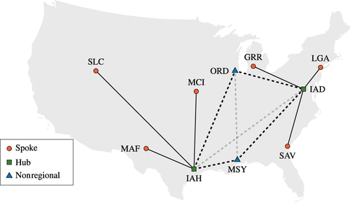
Note. Solid line, Mesa; dashed line, United Airlines.
3.4. Markets
We consider eight market types that are relevant for regional airlines: hub to hub, spoke to spoke, hub to NR (and vice versa), hub to spoke (and vice versa), and spoke to NR (and vice versa). We do not consider NR-to-NR markets because these are very rarely served by regional flights. Table 1 shows the relative sizes of each type of market for the major regional airlines in the United States, using data from the Bureau of Transportation Statistics (2023c). The first column is the regional airline’s IATA code, whereas the second column is the code of the corresponding mainline. The last column, “Market size,” reports the total number of passengers carried in the reference period (quarter 2 of 2022). All other columns report, for each row corresponding to a regional-mainline combination, the number of passengers belonging to a given market type as a percentage of the total market size of that regional-mainline combination. For each market type, the data are further decomposed by the number of segments that make up the passenger itinerary. For example, in the network depicted in Figure 1, a nonstop passenger from MAF to IAH would count toward the spoke-to-hub markets and one segment. A passenger flying from MAF to ORD with a connection at IAH would count toward the spoke-to-NR markets and two segments. The bold rows indicate the regional-mainline combinations that we use in our computational experiments (see Sections 6 and 7). In Appendices F to H, we evaluate the impact of our assumptions related to market characteristics; specifically, we relax the assumptions related to deterministic market sizes, itinerary attractiveness values, and average fares per itinerary.
|

Table 1. Percentage Market Sizes for the Main Regional Airlines Operating in the United States
| Hub to hub | Hub to NR | Hub to spoke | NR to hub | NR to spoke | Spoke to hub | Spoke to NR | Spoke to spoke | Quarterly | ||||||||||||||
|---|---|---|---|---|---|---|---|---|---|---|---|---|---|---|---|---|---|---|---|---|---|---|
| Segments | 1 | 2 | >2 | 2 | >2 | 1 | 2 | >2 | 2 | >2 | 2 | >2 | 1 | 2 | >2 | 2 | >2 | 1 | 2 | >2 | Market size | |
| 9E | DL | 1.2 | 0.3 | 0.1 | 0.4 | 0.4 | 19.7 | 1.4 | 0.1 | 0.3 | 0.4 | 20.4 | 1.1 | 19.5 | 1.5 | 0.1 | 20.4 | 1.2 | 7.1 | 4.2 | 0.1 | 2.8M |
| C5 | UA | 0.0 | 0.2 | 0.1 | 0.2 | 0.4 | 17.3 | 1.7 | 0.1 | 0.1 | 0.3 | 27.4 | 1.9 | 17.4 | 1.8 | 0.1 | 27.2 | 2.1 | 0.0 | 1.7 | 0.1 | 642.7K |
| G7 | UA | 0.1 | 0.6 | 0.0 | 0.6 | 1.4 | 23.2 | 0.4 | 0.0 | 0.4 | 1.0 | 22.9 | 1.1 | 23.4 | 0.4 | 0.1 | 21.8 | 1.4 | 0.0 | 1.4 | 0.0 | 389.7K |
| MQ | AA | 0.0 | 0.2 | 0.0 | 0.3 | 0.3 | 14.9 | 2.0 | 0.1 | 0.3 | 0.3 | 24.2 | 1.4 | 14.6 | 2.0 | 0.1 | 24.3 | 1.6 | 8.5 | 4.7 | 0.1 | 2.8M |
| OH | AA | 0.1 | 0.3 | 0.0 | 0.4 | 0.4 | 17.5 | 1.5 | 0.2 | 0.3 | 0.4 | 24.6 | 1.2 | 17.3 | 1.5 | 0.2 | 24.7 | 1.4 | 0.2 | 7.9 | 0.0 | 2.9M |
| OO | AA | 0.0 | 0.1 | 0.0 | 0.3 | 0.2 | 12.2 | 1.9 | 0.1 | 0.3 | 0.2 | 25.6 | 1.9 | 12.1 | 2.1 | 0.1 | 26.6 | 2.1 | 10.9 | 3.2 | 0.1 | 1.7M |
| OO | AS | 6.0 | 0.5 | 0.0 | 0.7 | 0.1 | 22.2 | 0.7 | 0.0 | 0.5 | 0.1 | 3.9 | 0.3 | 21.9 | 1.3 | 0.0 | 4.8 | 0.7 | 35.4 | 0.9 | 0.0 | 971.7K |
| OO | DL | 0.2 | 0.2 | 0.1 | 0.5 | 0.4 | 19.9 | 3.6 | 0.1 | 0.1 | 0.4 | 19.5 | 2.1 | 20.0 | 3.6 | 0.2 | 19.8 | 2.4 | 0.1 | 6.1 | 0.5 | 3.2M |
| OO | UA | 0.1 | 0.4 | 0.1 | 0.2 | 0.2 | 20.9 | 3.4 | 0.1 | 0.1 | 0.2 | 20.4 | 1.0 | 20.4 | 3.6 | 0.2 | 21.1 | 1.5 | 0.0 | 5.9 | 0.3 | 3M |
| PT | AA | 0.0 | 0.2 | 0.0 | 0.2 | 0.5 | 8.5 | 0.7 | 0.1 | 0.1 | 0.5 | 33.9 | 2.6 | 8.6 | 0.7 | 0.1 | 33.4 | 2.7 | 5.0 | 2.5 | 0.0 | 815.2K |
| YV | AA | 0.0 | 0.1 | 0.0 | 0.3 | 0.3 | 16.0 | 0.6 | 0.1 | 0.2 | 0.3 | 30.1 | 1.4 | 15.9 | 0.6 | 0.1 | 29.6 | 1.7 | 0.0 | 2.7 | 0.0 | 903.3K |
| YV | UA | 0.1 | 0.3 | 0.0 | 0.6 | 0.4 | 28.1 | 0.3 | 0.0 | 0.3 | 0.2 | 18.3 | 0.7 | 28.0 | 0.4 | 0.0 | 18.0 | 1.0 | 0.5 | 2.7 | 0.0 | 752.4K |
| YX | AA | 0.8 | 0.2 | 0.0 | 1.3 | 0.4 | 26.1 | 1.2 | 0.0 | 1.1 | 0.4 | 11.7 | 1.1 | 26.0 | 1.4 | 0.1 | 12.0 | 1.0 | 11.2 | 4.0 | 0.0 | 1.9M |
| YX | DL | 6.3 | 0.0 | 0.0 | 2.3 | 0.5 | 28.9 | 0.6 | 0.0 | 2.5 | 0.4 | 8.0 | 0.6 | 28.8 | 0.8 | 0.0 | 7.9 | 0.6 | 10.6 | 1.2 | 0.0 | 1.2M |
| YX | UA | 0.0 | 0.2 | 0.0 | 0.5 | 0.5 | 30.5 | 0.2 | 0.0 | 0.2 | 0.3 | 14.5 | 0.7 | 29.5 | 0.2 | 0.0 | 13.9 | 0.9 | 5.2 | 2.7 | 0.0 | 1.1M |
| ZW | UA | 0.0 | 0.0 | 0.0 | 0.2 | 0.2 | 12.8 | 0.5 | 0.0 | 0.1 | 0.2 | 29.8 | 1.8 | 12.5 | 0.5 | 0.0 | 29.7 | 2.2 | 6.1 | 3.2 | 0.0 | 574.1K |
Notes. The last column reports the total number of passengers using the regional-mainline combination in the first two columns. All other columns report the market size of each market type as a percentage of the total market size of that regional-mainline combination. Therefore, the sum of values in columns (2)–(20) for any given row is 100.
3.5. Paths
We assume that for each market, all passengers who use at least one regional flight follow the same path. For example, in the network shown in Figure 1, the MAF-ORD market can be served via the MAF-IAH-ORD and MAF-IAH-MSY-IAD-ORD paths, but the former is much more popular. In fact, typically only one path for each market captures almost all of the demand served by the regional airline. For example, when considering mainline UA and regionals YV and YX, 91.29% of all passengers take the most popular path; when aggregating on a market-by-market basis, the median percentage of passengers taking the most popular path is 100%. In our model, we assume that all passengers use the most popular path for each market. However, note that our model allows the passengers to choose from all the different itineraries corresponding to that popular path, with varying departure and arrival times of the flight(s) in those itineraries.
3.6. Passenger Connection Times
We assume that all passengers in the same market follow the same itinerary if they meet the following two conditions: (a) their itinerary includes one regional flight and one mainline flight, and (b) they take the same regional flight. For example, passengers on the MAF-IAH-ORD path who take a regional MAF-IAH flight with Mesa Airlines that departs at 08:00. and arrives at 10:00 will all continue their journey on the same mainline IAH-ORD flight. If there are mainline flights departing at 10:50, 11:50, and 12:50 on segment IAH-ORD, then all MAF-IAH-ORD passengers arriving on the Mesa flight to IAH at 10:00 will take the 10:50 departure to ORD, assuming that the 50-minute connection time is feasible and more desirable for passengers than the 110- or 170-minute connection times. In Appendix I, we study the impact of varying the minimum connection time that makes a connection feasible for passengers.
3.7. Number of Connections
We assume that all itineraries have at most two segments. Indeed, Table 1 shows that only a tiny fraction of passengers use itineraries with more than two segments. When considering the mainline UA and the regionals YV and YX, only 2.36% of passengers use itineraries with more than two segments. The two-segment itineraries can be of two types: both segments served by regionals or one segment served by a regional airline and the other by the mainline. In our model, we directly include all markets served by two-segment itineraries that involve one regional segment and one mainline segment. On the other hand, we split every market served by two-segment itineraries involving two regional segments into two separate markets. Each of these two markets is modeled to be served by a single-segment itinerary. For mainline UA and regionals YV and YX, only 1.33% of passengers use an itinerary with more than one segment operated by regional airlines. In Appendix J, we show that this simplification, which allows us to model revenue on a segment-by-segment basis, only minimally affects the results.
4. Mathematical Models
In this section, we develop an integrated single-day scheduling model for the combined problem of frequency planning, timetable development, and fleet assignment for a network of one or more regional airlines that support a single mainline. In Section 4.1, we formulate the FTFA as an extended mixed-integer programming (MIP) model called the master problem. In Section 4.2, we tackle the problem of generating promising missing variables when not all of them are enumerated in the master problem. We decompose the problem of generating such variables on a segment-by-segment basis, and, for a given segment, we present an auxiliary MIP model called the pricing subproblem. In Section 5, we present a column generation algorithm to solve the master problem using the segment-by-segment pricing subproblems. Table 2 summarizes the notation used throughout this section.
|
Table 2. Sets, Parameters, and Decision Variables Used to Formulate the Master Problem (Section 4.1) and the Pricing Subproblem (Section 4.2)
| Set | Description |
|---|---|
| D | Set of airports served by the regional airline. |
| L | Set of segments served by the regional airline. |
| T | Set of periods in the planning horizon. |
| Valid departure periods for flights in segment . | |
| Departure times for flights in segment in a given segment schedule. | |
| Set of time periods in the extended time horizon; it includes the planning horizon and the period after that. | |
| Q | Set of all markets included in the model. |
| Set of markets whose itineraries include a flight in segment . | |
| A | Set of aircraft types. |
| Aircraft types that can operate segment . | |
| Valid departure periods for flights in that can be operated by an aircraft of type . | |
| Set of airports where an aircraft of type can operate. | |
| Set of segments that can be operated by an aircraft of type . | |
| Aircraft types that can operate a flight in segment departing in period . | |
| Set of aircraft types that can operate at airport . | |
| Set of all feasible segment schedules. | |
| Set of all feasible schedules for segment . | |
| Schedules for segment , containing a flight departing in period and operated by an aircraft of type . | |
| Schedules for segment , containing a flight operated by an aircraft of type and departing at some time in the set whose sum of arrival time and turnaround time corresponds to period . |
| Parameter | Description |
|---|---|
| Size of market . | |
| Attractiveness of an itinerary containing a flight in segment departing at time for passengers of market . | |
| Shadow attractiveness of an itinerary containing a flight in segment departing at time for passengers of market . | |
| Attractiveness of the outside option for passengers of market . | |
| Adjusted attractiveness of an itinerary containing a flight in segment departing at time for passengers of market . | |
| Adjusted attractiveness of the outside option for passengers of market . | |
| Fare for a passenger in market flying on segment at time . | |
| Cost of operating a flight in segment departing at time using an aircraft of type . | |
| Number of periods needed for an aircraft of type to be ready for the next flight after it flies on segment ; it includes the flight time from i to j and the turnaround time at j. | |
| Fleet size for aircraft type . | |
| Seating capacity of aircraft type . | |
| Minimum number of periods between two consecutive departures for segment . | |
| Minimum frequency for segment . | |
| Maximum frequency for segment . | |
| Takes value one if and only if an aircraft of type can operate a flight at time on segment when performing incremental retiming. | |
| Maximum load factor for segment . | |
| Profit earned when operating the flights in segment schedule . | |
| Variable | Description |
| Takes value one if and only if a flight in segment departing in period is operated by an aircraft of type . | |
| Number of passengers of market taking a flight at time in segment . | |
| Number of passengers of market taking the outside option. | |
| Takes value one if and only if we operate the segment schedule . | |
| Number of aircraft of type available at airport at the beginning of period . |
4.1. Master Problem
In this section, we propose an extended MIP formulation for network-wide schedule optimization. Given a pair of airports, i and j, connected by regional flights, that is, as per the notation of Table 2, we define a segment schedule S between i and j as a sequence of pairs in which t is the departure time of a flight from i to j using an aircraft of type a. Segment schedules are sufficient to build a complete, network-wide schedule for a regional airline because they keep track of all aircraft movements on the segments operated by the airline. Denote by the set of all feasible segment schedules for a given segment and by the set of all feasible segment schedules. We introduce two sets of decision variables using the notation presented in Table 2. First, the variables take the value one if and only if the regional airline decides to operate the segment schedule . Second, the variables represent the number of aircraft of type that are available at the airport at the beginning of the period .
Figure 2 presents an example of a solution to the master problem for the subnetwork containing hub IAH and spokes MAF, SLC, and MCI of the network presented in Figure 1 and using a time discretization of 30 minutes. The solution uses two aircraft ( and ) of the same aircraft type a and builds six schedules, one for each hub-to-spoke or spoke-to-hub segment, which are listed in the legend below the figure. For example, the schedule selected in the solution () is because there are two flights from IAH to SLC, whose start times are highlighted with strong purple squares at 11:30 using aircraft and at 14:00 using aircraft . Note that the variables take the value two for because both aircraft are stationed at the hub during these periods, the value one for , and the value zero during other periods. The variables work analogously for all other airports and periods.

Note. The solution uses two aircraft ( and ) of the same type and builds six segment schedules, one for each hub-to-spoke and spoke-to-hub segment.
The master problem formulation reads as follows.
The Objective Function (1a) maximizes the total profit from the chosen set of segment schedules. Constraints (1b) ensure that exactly one segment schedule is selected for each segment operated by the regional airline. Constraints (1c) ensure that no more aircraft of each type are used than are available. Constraints (1d) link the variables y and w that impose flow conservation at each airport in each period and for each aircraft type. Constraints (1e) ensure that the aircraft are correctly positioned at the end of the planning horizon to ensure that the same schedule can be repeated.
We remark that in Model (1a)–(1g), the profit of each segment schedule is independent of whether other regional segment schedules are selected. This is enabled by our simplification (first stated at the end of Section 3) of splitting markets served by two-segment itineraries in which both segments are operated by a regional airline into the two corresponding single-segment markets. This simplification makes our formulation more tractable, and the results in Appendix J demonstrate that it only minimally affects results.
Note that for a given segment , the number of variables is exponential in the number of periods. Furthermore, in the worst case, the number of feasible solutions of (1a)–(1g) is exponential in the number of segments.
Enumerating all feasible schedules in would be prohibitively expensive because of the size of the set. Moreover, most feasible schedules are not attractive from a commercial point of view. These observations suggest that an appropriate solution method for the master problem should initially discard most segment schedules and use a pricing subproblem to identify promising ones. At the same time, dual information from the continuous relaxation of the master problem should be used in the pricing subproblem to ensure that the resulting segment schedules work well when used jointly. To achieve this goal, in Section 4.2, we introduce a family of MIPs, one for each segment , whose optimal solutions correspond to feasible segment schedules. Each such schedule has an associated reduced cost, which, if positive, indicates that the schedule should be included in the master problem.
In summary, Formulation (1a)–(1g) is challenging to solve because of the exponentially many variables y in each segment. However, as demonstrated in Section 6, this formulation has an especially tight continuous relaxation. Furthermore, we develop an exact column generation procedure and a novel acceleration technique, presented in Section 5, that efficiently solve the continuous relaxation. Ultimately, a tight continuous relaxation and an efficient column generation procedure together yield high-quality solutions in short runtime budgets (at most three hours) for planning problems at the scale of real-world airline networks.
4.1.1. Master Problem Extensions.
We present extensions to the master problem model that can be used to capture additional network-level requirements. See Appendix A for a detailed overview of each extension, where we describe the eventual new constraint(s) needed and how they affect the dual structure of Formulations (1a)–(1g).
Route selection. By relaxing the Equality Constraint (1b) into a less-than-or-equal-to () constraint, one can incorporate route selection decisions. The resulting model can decide not to assign any schedule to some segments, which corresponds to not operating the segments.
Airport slot restrictions. Many airports limit the number of flight operations that an airline can have at that airport during each period to the number of slots assigned to that airline. Our model allows limiting the number of flights departing from or arriving at each airport during some or all periods to account for such slot constraints.
Mainline capacity. Passengers on two-segment itineraries can take the regional flight only if they can get a seat on the mainline flight. Given the list of mainline flights with the respective capacities that are expected to be available to regional passengers, we can impose the requirement that the chosen regional flights must allow for a feasible continuation of the itinerary on the mainline carrier’s network.
Average aircraft utilization. Factors not captured endogenously by our model (e.g., planned maintenance of the aircraft) affect aircraft utilization. To ensure that the results correspond to real-world conditions, we cap the average utilization of each fleet type to that in the actual schedules in all computational experiments.
4.2. Pricing Subproblem
In this section, we present the pricing subproblem. The variables are the columns that we generate in our column generation algorithm. In particular, our algorithm uses dual information from the continuous relaxation of (1a)–(1g) to generate promising segment schedules. In the following, we denote the continuous relaxation of Formulation (1a)–(1g) as [MP]. Let and , respectively, be the dual variables associated with Constraints (1b) and (1d) in [MP].
The pricing subproblem can be decomposed segment by segment, that is, for each , one can search for promising segment schedules in the set . The set of promising schedules for the master problem is the union of the sets of promising schedules obtained segment by segment. Note that, given a segment , using the notation presented in Table 2, the reduced cost of a schedule is
Let be the number of passengers of market q taking the flight in segment schedule departing in period t. Using the notation presented in Table 2, the profit associated with schedule S is
We denote the following quantities with and :
Note that f and are identical as defined in (4), but this is not necessarily the case when using the model extensions presented in Section 4.1.1. Appendix A explains how to amend the definitions of and for each considered extension. With this notation, we can write the reduced cost of S in the following way.
The pricing subproblem finds, for each segment connected by regional flights, a feasible segment schedule with the Highest Reduced Cost (5). The output of this process of solving the pricing subproblem will be not only a segment schedule S, that is, a sequence of pairs in which t is the departure time of a flight from i to j using an aircraft of type a, but also a vector in which the component indexed by is the number of passengers of market flying on segment with a flight departure time t. The segment schedule can be used to calculate the total cost of operating flights from i to j, whereas vector is used to evaluate the revenue earned by selling tickets to passengers that use a flight in segment as part of their itinerary. To this end, we need a model that calculates the passenger flow given the segment schedule and fares. Therefore, a scheduling model aiming to maximize the reduced cost must integrate a passenger allocation model within it.
4.2.1. Passenger Allocation Model.
Determining how many passengers will take each scheduled flight is challenging because this number depends on passenger preferences, the entire offering of flights from i to j, other segments that are parts of itineraries containing segment , the available seating capacity on each flight, and the attractiveness of other travel alternatives (including not traveling at all). Following Wei, Vaze, and Jacquillat (2020), we use a general attraction model (GAM) to incorporate endogenous passenger choices and determine the resulting passenger flows.
Let be the set of scheduled departure times on segment in a given segment schedule, and let be the size of market q. Denote with , , and , respectively, the attractiveness, the shadow attractiveness, and the adjusted attractiveness of the itinerary containing a flight in segment with flight departure time in period t to passengers in the market q. Note that . The concept of shadow attractiveness was introduced by Gallego, Ratliff, and Shebalov (2015) to overcome the independence of irrelevant alternatives property of the multinomial logit model. In the GAM, the attractiveness of the itinerary is the exponential of a linear function of itinerary attributes, such as fare, time of day, travel time, connection time, and inconvenience (Barnhart, Fearing, and Vaze 2014). We refer the reader to Gallego, Ratliff, and Shebalov (2015) for more details on the GAM and to Wei, Vaze, and Jacquillat (2020) for more details on the adjusted attractiveness of an airline itinerary. Let be the attractiveness of the outside option. The outside option represents the aggregation of all alternatives available to a passenger that do not include flying with the regional airline under consideration. This may include traveling with flights from other airlines, traveling using other modes of transportation, or not traveling. Finally, is the adjusted attractiveness of the outside option. All attractiveness values are calculated based on real-world data, as explained in Appendix B.
In the absence of a tight seating capacity constraint, under the GAM, the number of passengers of market taking a flight from i to j with a flight departure time t is
When there is enough seating capacity, Expression (6) equals the number of passengers carried, and when the seating capacity constraint is tight, Expression (6) serves as an upper limit to the number of passengers carried.
4.2.2. Pricing Subproblem Formulation.
A mathematical formulation for the pricing subproblem for a given segment uses variables (, ), (, ), and (). Variable equals one if and only if the segment schedule includes a flight operated by an aircraft of type a departing in period t. and are the number of passengers in market q taking, respectively, a regional airline flight departing at time t or the outside option. The formulation is as follows.
The Objective Function (7a) maximizes the schedule’s reduced cost. Constraints (7b) ensure that the segment schedule does not use more aircraft than available in any time window of size . The time window’s size reflects the fact that the quickest way for an aircraft flying from i to j to be ready to fly again from i is, upon arriving at j, to turn around and fly back to i immediately. Constraints (7c) define the demand for each flight to be proportional to its adjusted attractiveness. Constraints (7d) ensure that the sum of the number of passengers taking the various alternatives (including the outside option) in a market is equal to the total passenger demand in that market. Constraints (7e) ensure that the available seats on each flight are enough to carry all passengers taking that flight.
Constraints (7c)–(7e), first introduced by Gallego, Ratliff, and Shebalov (2015), allow incorporating the nonlinear GAM through a small family of linear inequalities. This is commonly known as the sales-based linear program (SBLP) reformulation of the discrete choice models that belong to the GAM family. This approach, first applied to airline scheduling by Wang, Klabjan, and Shebalov (2014), allows us to model the pricing subproblem as a compact MIP model, compared with techniques that used an exponential number of constraints (Méndez-Díaz et al. 2014) or conic integer programming (Sen, Atamtürk, and Kaminsky 2018).
4.2.3. Pricing Subproblem Extensions.
In the following, we describe possible modeling extensions that capture additional real-world constraints in the pricing subproblem model. The corresponding new parameters are also reported in Table 2.
Padding between consecutive flights. Marketing and operational considerations often suggest that consecutive flights on the same segment should not be scheduled to depart too close to each other. Our model can take this requirement into account through the following constraint.
(8)Minimum and maximum number of flights. A planner can impose hard limits on the minimum and maximum number of flights on a segment, adding the following constraint.
(9)If and both values are equal to the number of flights in segment in the current airline schedule, the planner forbids frequency changes and only makes fleet assignment and retiming decisions.
Incremental flight retiming. The planner can decide to allow only incremental retiming of the currently operated schedule. For example, the planner might allow flight departure times to change by no more than 30 minutes compared with the currently operated schedule. In our model, this can be achieved by forcing variable to take the value zero if departure time t falls outside the allowed ranges.
Maximum load factor. Flight load factors are influenced by many decisions, especially related to revenue management, that are outside the scope of our optimization model. The decision maker can specify a maximum load factor for each segment by adding the following constraint to ensure that our model is not too optimistic in assigning passengers to flights.
(10)Aircraft type–dependent attractiveness and fares. The attractiveness of an airline itinerary to a passenger can sometimes be influenced by the types of aircraft used to operate its flights. Moreover, an airline might consider charging different fares for the same itinerary as a function of the aircraft type. Such situations can be modeled by defining new fare parameters and to replace and , new attractiveness parameters and to replace and , and new passenger allocation decision variables to replace , each with an additional index . Moreover, the Objective Function (7a) becomes
Finally, the following constraints replace (7c)–(7e):
We note that several other extensions only involve variable fixing. For example, some airlines use banked hubs; that is, mainline and regional flights arrive and depart in waves at the hubs, with a wave of departing flights following a wave of flight arrivals. Scheduling arrivals or departures within such bank windows corresponds to fixing to zero those variables that correspond to out-of-bank arrival or departure times.
5. Column Generation Algorithm
In this section, we explain how we solve the continuous relaxation [MP] to optimality and how we use its solution to produce a high-quality solution to the integer version of the master problem.
The algorithm is initialized by solving a restricted [MP] with a single dummy column . This dummy column has a coefficient of one in the Inequalities (1b), does not appear in (1d), and has a large negative objective coefficient. Adding the dummy column ensures that [MP] is always feasible. If in the optimal solution to [MP], then the problem is infeasible.
A new segment schedule can improve the objective function of [MP] if its reduced cost is strictly positive. Therefore, in each iteration of the algorithm, we solve one pricing subproblem for each segment and add to the restricted [MP] all the y variables associated with positive-reduced-cost segment schedules. We note that each pricing subproblem can produce multiple positive-reduced-cost columns; to this end, we instruct the MIP solver used to optimize the subproblem to keep a list of all visited feasible solutions, and we add all feasible segment schedules with positive reduced cost to the restricted [MP]. When all subproblems prove that no positive-reduced-cost segment schedule exists (i.e., the optimal solutions of all pricing subproblems have a nonpositive objective value), the incumbent solution to the restricted [MP] is optimal for the [MP]. At that point, we resolve the restricted [MP] but with Integrality Constraints (1f) and (1g) reinstated. In other words, we solve (1a)–(1g) using only the generated columns. The procedure presented in this section has been called a restricted master heuristic or a price-and-branch algorithm (Joncour et al. 2010, Desrosiers and Lübbecke 2011).
5.1. Heuristic Column Generation
In principle, there is no need to solve the pricing subproblems to optimality, and any feasible solution with positive reduced cost, when added to the column pool, can improve the objective function of the restricted [MP]. However, special care is needed when the solution to a subproblem is not optimal. For any given segment and period , for the SBLP reformulation to work correctly, either (7e) is tight, all Constraints (7c) are tight, or both. This condition always holds for optimal solutions to the pricing subproblem. However, in a suboptimal solution to the pricing subproblem, this condition might be violated for some . Consider such a suboptimal solution where, for the given and , the variables take the values and . Then, it is possible to set some of the variables to a value higher than and, correspondingly, set some of the variables to a value lower than while still satisfying Constraints (7c)–(7e). The resulting new solution to the pricing subproblem would have a better objective value. Therefore, if we used the suboptimal solution to a pricing subproblem to build a segment schedule as a new column in the restricted [MP], its objective coefficient in the restricted [MP] could be wrong because it is calculated using a number of passengers that does not follow the GAM.
To avoid such erroneous objective coefficients in the restricted [MP], we must ensure that for any segment schedule defined by variables , the remaining variables (namely, and especially ) maximize the objective function of the pricing subproblem across all solutions with that segment schedule. To compute with GAM-consistent passenger allocation, one can fix the variables and resolve (7a)–(7h) to optimality (we call this procedure “z-fixing”). This transition from a feasible solution to a pricing subproblem that does not follow the GAM to one that does, by definition, cannot decrease the reduced cost.
In terms of the overall implementation of column generation, this issue is linked to the classical question of whether to add single or multiple columns at each pricing iteration. In most cases, adding multiple columns improves the convergence of the column generation algorithm and the quality of the restricted master heuristic solution. However, adding more than one column usually does not involve any additional computation, whereas in our case, each potentially suboptimal column requires running the z-fixing procedure.
This led to three different pricing strategies that we experimented with. In the first strategy, we solve the pricing subproblem, and we instruct the MIP solver to stop as soon as it finds the first positive-reduced-cost solution. We add that single column to the restricted [MP], potentially after running the z-fixing procedure in case the pricing solution is suboptimal. The second strategy involves solving the pricing subproblem to optimality. In this case, the corresponding solution is guaranteed to follow the GAM, and no z-fixing is required. In the third strategy, we solve the pricing subproblem to optimality and inspect all the feasible integer solutions encountered by the MIP solver. We run a z-fixing procedure for each suboptimal integer solution and add all positive-reduced-cost integer solutions to the column pool. We conducted a preliminary experiment to determine the most effective strategy, and the results showed that the third strategy outperforms the others. This is because the z-fixing procedure is quick and does not significantly impact the algorithm’s overall time, but enriches the column pool. Therefore, all the results in this paper follow the third strategy.
5.2. Approximating an Upper Bound on the Reduced Cost
We describe how to derive an upper bound on the reduced cost of a column by solving a relaxation of the pricing subproblem using dynamic programming. This procedure can result in two cases. On the one hand, if the upper bound is negative, then no positive-reduced-cost columns exist. On the other hand, in producing the bound, the procedure can build a segment schedule that can be added to the column pool of the reduced [MP]. Computational experiments show that the DP usually produces high-quality columns and helps to improve the overall convergence of the column generation algorithm.
To apply DP, we first aggregate all the markets whose itineraries include a flight in segment , and therefore, the aggregate market size is given by . To overestimate the reduced cost, we assume that in any given period , all passengers have the highest fare across all markets , given by . We also relax the assumption of GAM-following market shares. Instead, we assume that the passengers are allocated across different flights in a segment schedule in a way that maximizes its reduced cost. In other words, we assume that the airline can decide how many passengers to carry on each flight in the segment schedule while still satisfying the aircraft capacity constraints for all individual flights and respecting the aggregate market size limit. Finally, we disregard Constraints (7b) and, if applicable, Constraints (9). This is consistent with obtaining an overestimation of the reduced cost of a segment schedule. However, we note that Constraints (7b) are unlikely to be active anyway because the fleet size is usually much larger than the number of aircraft needed to operate a profitable single-day schedule on a single segment. We define a “relaxed segment schedule” (RSS) as a segment schedule that satisfies all constraints other than (7b) and (9). We define the “relaxed reduced cost” (RRC) of an RSS as its reduced cost calculated under these modifications.
Denote by the highest RRC across all RSS whose first flight does not depart before when the aggregate market size is . Then, —the highest RRC across all RSS—constitutes an upper bound on the maximum reduced cost across all segment schedules for that segment .
We compute using DP. Recall that is the set of valid flight departure times for flights in segment . We denote by the first valid departure period that is not before .
Then, the Bellman equation of our DP algorithm is as follows.
The top line of (11) refers to the case where no flight is scheduled at time t. The bottom line defines the maximum RRC achievable when operating a flight departing at time t using the best possible aircraft type a and carrying the best possible number of passengers . This RRC is the sum of two components: the first one, from the flight departing at time t, is ; the second one, , is the best possible RRC achieved by flights departing at time or later and carrying at most passengers. We can set if the constraints (8) are not used.
We note that in Recursion (11), the first argument to function always strictly increases. Therefore, to initialize the algorithm, we provide values for all t values greater than the last valid departure period.
Value appears as a constant in the pricing subproblem’s Objective Function (7a).
The table for the DP defined above has a size proportional to . However, changing the number of passengers carried by one does not significantly impact the total reduced cost of a segment schedule. As a result, a one-passenger resolution is often unnecessary to obtain an accurate approximation of the reduced cost of a segment schedule. We propose to reduce the size of the DP table by dividing the set into buckets of size B; therefore, we only consider values M if they are multiples of B or if . However, we note that the RRC computed using this approximation is no longer guaranteed to be an upper bound on the maximum reduced cost of a segment schedule for all .
The output of the DP algorithm is an RSS S and its approximate RRC . To determine whether S is feasible and, if so, what its exact reduced cost is, we solve the Model (7a)–(7h) fixing variables to the value one if or to zero otherwise. When the resulting segment schedule is feasible and has a positive actual reduced cost, we add the corresponding column to the pool. Otherwise, we must solve (7a)–(7h) directly to determine whether any positive-reduced-cost columns exist.
5.3. Acceleration Strategies
We present three additional strategies to speed up the column generation algorithm.
5.3.1. Dual Stabilization.
We counteract the tendency of column generation algorithms toward dual variable oscillations and tailing-off (see, e.g., Vanderbeck and Wolsey 1996) by setting Gurobi’s Method parameter to BARRIER (value 2) when solving the restricted [MP] and by disabling the crossover procedure (Bixby and Saltzman 1994) by setting Gurobi’s Crossover parameter to zero. We call this approach implicit dual stabilization because Pessoa et al. (2018) have remarked that interior point methods, such as the Barrier algorithm, have “an inherent stabilization feature.” We also tried explicit dual stabilization; in particular, we implemented the dual smoothing method of Pessoa et al. (2018), but we did not get any further computational gains.
5.3.2. Selecting Which Subproblems to Solve (Subproblem Aging).
After a few dozen column generation iterations, most subproblems do not return any positive-reduced-cost solutions for many iterations, and eventually, many of them never will. We define cold subproblems as those that do not generate positive-reduced-cost columns in a given iteration. Other subproblems are defined as hot. When, in some iteration, more than half of the subproblems are cold, we enter a shortcut mode. In shortcut mode, we solve the subproblems in decreasing order of the number of positive-reduced-cost columns they produced during the previous iteration. We stop solving subproblems as soon as one fails to produce positive-reduced-cost columns after at least one such column was produced in the current iteration. At that point, we solve the restricted [MP] again and move on to the next column generation iteration. The main idea behind this strategy is to attempt to solve hot subproblems only and resort to solving the cold ones at the end of the algorithm to prove that no more positive-reduced-cost columns exist.
5.3.3. Breaking Symmetry in the Subproblems.
When solving the pricing subproblem for a segment , the objective function coefficients of variables x and z depend on passenger fares , operating costs , and the dual values. Although the fares and operating costs could vary between periods t, in practice, some of them could be identical. For example, operating a flight at 10:00 might cost the same as at 10:15. The duals are also likely to take only a few different values, and most of them take the value zero because they correspond to nonbinding primal constraints. Indeed, in our experiments, we observed that the pricing subproblem is affected by symmetry. For example, operating a flight at 08:00 might yield the same reduced cost as operating it at 08:15, 08:30, etc. To break this symmetry, we add a negligible amount of noise to all fares ; more precisely, we add a Gaussian noise with mean zero and standard deviation . Computational experiments confirmed that instances that only differ in whether the noise was added to the fares produce primal and dual bounds that are indistinguishable for practical purposes.
6. Computational Results
In this section, we present the results of our computational experiments to evaluate the impact of the main algorithmic design choices. We consider seven instances obtained using real-world data for the three largest regionals that support United Airlines: Mesa Airlines (YV), Republic Airways (YX), and SkyWest Airlines (OO). This combination of mainline carriers and regionals gives rise to one of the largest instances that can be built from publicly available data. We build one instance for each possible combination of one, two, and three regional airlines. Table 3 reports the main network characteristics of each instance: the number of hub and spoke airports, the number of segments operated, the number of flights flown, the number of markets served, and the number of individual aircraft and aircraft types used. This data were obtained from the Bureau of Transportation Statistics (2023a, b, c) for June 29, 2022 (which was a Wednesday). The largest joint instance (VY + YX + OO) involves operations at 156 airports throughout the continental United States, with more than 3,000 markets (that is, more than 3,000 unique origin-destination pairs between which passengers want to travel), and optimizes a fleet of almost 350 aircraft. When creating instances combining multiple regionals, the listed numbers of flights and aircraft in the combined instance are always simple sums of the corresponding values for the individual regionals. However, other characteristics, namely, hubs, spokes, segments, markets, and aircraft types, sometimes overlap, resulting in the combined characteristics being different from the simple sums of the parts. Appendix B provides more details on our setup of the case study and data preprocessing steps, whereas Appendix C provides detailed computational statistics.
|
Table 3. Main Network Characteristics of the Considered Instances
| Instance | Hubs | Spokes | Segments | Flights | Markets | Aircraft types | Aircraft |
|---|---|---|---|---|---|---|---|
| YV | 2 | 28 | 64 | 90 | 230 | 2 | 38 |
| YX | 2 | 30 | 70 | 128 | 206 | 2 | 48 |
| OO | 5 | 124 | 416 | 784 | 2,810 | 3 | 260 |
| YV + YX | 4 | 44 | 134 | 218 | 454 | 3 | 86 |
| YV + OO | 6 | 145 | 518 | 874 | 2,819 | 4 | 298 |
| YX + OO | 6 | 146 | 488 | 912 | 2,721 | 4 | 308 |
| YV + YX + OO | 7 | 149 | 534 | 1,002 | 3,312 | 5 | 346 |
The tested algorithmic design choices are as follows.
Barrier. Setting Gurobi’s Method parameter to value BARRIER, as explained in Section 5.3.1.
SP Aging. Cutting short some column generation iterations when the likelihood of producing new positive-reduced-cost columns later in the same iteration is low, as explained in Section 5.3.2.
Noise. Adding a tiny amount of noise to fares to break the symmetry in the subproblem, as explained in Section 5.3.3.
DP. Using the dynamic programming algorithm introduced in Section 5.2 and solving the MIP Formulation (7a)–(7h) only if the DP algorithm does not produce any positive-reduced-cost column.
Table 4 shows the results of an ablation study comparing five configurations. In the “base” configuration, all algorithmic improvements are active. In the other four configurations, we disable one improvement at a time to evaluate how much the corresponding algorithm’s performance differs from the base configuration. We ran all experiments on a cluster with Intel Xeon CPUs running at 2.6 GHz. The algorithms were coded in C++, and we used Gurobi 9.0.0 as the linear and integer programming solver with a time limit of three hours (unless explicitly stated otherwise). For the DP algorithm, we used a bucket size of .
|
Table 4. Ablation Study Results
| Base | No DP | No barrier | No SP aging | No noise | ||||||
|---|---|---|---|---|---|---|---|---|---|---|
| Instance | Gap (%) | Time (seconds) | Gap (%) | Time (seconds) | Gap (%) | Time (seconds) | Gap (%) | Time (seconds) | Gap (%) | Time (seconds) |
| YV | 0.11 | 52.80 | 0.09 | 703.75 | 0.10 | 4,602.45 | 0.11 | 277.76 | 0.10 | 1,042.75 |
| YX | 0.20 | 884.05 | 0.20 | 1,883.55 | 0.20 | 1,506.19 | 0.20 | 1,696.42 | 0.20 | 2,541.12 |
| OOa | 0.00 | 10,800.00 | 0.00 | 10,800.00 | 0.00 | 10,800.00 | 0.01 | 10,800.00 | — | 10,800.00 |
| YV + YX | 0.17 | 1,115.75 | 0.13 | 6,051.81 | 0.14 | 1,742.86 | 0.19 | 1,666.04 | 0.14 | 8,481.55 |
| YV + OOb | 0.08 | 10,800.00 | — | 10,800.00 | — | 10,800.00 | 0.11 | 10,800.00 | — | 10,800.00 |
| YX + OOc | 0.12 | 10,800.00 | — | 10,800.00 | — | 10,800.00 | — | 10,800.00 | — | 10,800.00 |
| YV + YX + OOd | 0.09 | 10,800.00 | — | 10,800.00 | — | 10,800.00 | — | 10,800.00 | — | 10,800.00 |
aColumn generation runtime: Five hour, seven minutes.
bColumn generation runtime: 15 hours, 39 minutes.
cColumn generation runtime: Five hours, 38 minutes.
dColumn generation runtime: 11 hours, nine minutes.
In the four instances that involved OO, the column generation algorithm did not terminate within the time limit. In these cases, we ran the final MIP (which solves almost instantaneously) with the columns generated before the three-hour timeout. However, we could not always obtain a feasible MIP solution. The dashes in Table 4 represent cases in which the columns generated in the three-hour limit produced an infeasible MIP.
All gaps are computed relative to the optimal solution of continuous relaxation [MP]. When such a solution was not available within the three-hour time limit, we ran the column generation algorithm until the continuous relaxation [MP] was optimally solved. We note that, under a hard time budget constraint, an upper bound on the cost of the optimal [MP] solution can be obtained, as explained in Appendix D.
The impact of our algorithmic improvements is twofold. In smaller instances (which do not involve OO), they cause a large reduction in computational times, up to 87× compared with “no barrier,” 5× compared with “no SP aging,” 20× compared with “no noise,” and 13× compared with “no DP.” The greatest improvements are for YV, whereas the improvements are moderate (1.5 × –7.6×) for YX and YV + YX. All configurations show extremely small gaps (≤0.20%) that demonstrate the strength of our extended formulation.
In larger instances, the column generation algorithm without the algorithmic improvements is often unable to obtain even a feasible solution within the three-hour time limit. For example, the “base” configuration is the only one producing a feasible integer solution in the YX + OO and YV + YX + OO instances. The reason is that its more efficient column generation procedure allows us to complete more pricing rounds, thus generating more columns and enabling the MIP solver to build a feasible solution. The “base” configuration not only obtains feasible solutions to all four hard instances within the three-hour time limit, but the solutions are also not more than away from the optimum in all cases. In summary, our algorithmic improvements provide a 1.5× to 87× runtime speedup for smaller instances and produce near-optimal solutions for larger instances for which the algorithm without the improvements is often unable to find even a feasible solution.
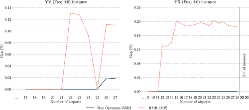
The gap between our restricted master heuristic (RMH) approach and the optimal solution of the continuous relaxation [MP] is generally small (as mentioned, it is never larger than 0.20%). However, it is not clear what part of the gap is due to the suboptimality of the RMH solution and what part is the continuous relaxation gap (that is, the gap between the optimal integer solution and the optimal solution to the continuous relaxation [MP]). To answer this question, we produced several smaller instances that can be solved to optimality by complete column enumeration. We started with the YV and YX instances, truncated them by removing airports (in decreasing order of status quo total daily frequency), and solved the truncated instances via column enumeration. We did not impose a time limit and allowed the enumeration algorithm to run for several days, which led to the true integer optimal solution of all the truncated YV instances (up to the one with all airports) and of the truncated YX instances with up to 28 out of 30 airports. For the YX instances with 29 and 30 airports, the enumeration procedure ran out of available memory (32 GB). Across all 55 truncated instances where an optimal solution was available, our RMH approach found the optimum in all but two cases—YV with 26 and 27 airports. In these two cases, the gap between the RMH solution and the optimum of the continuous relaxation [MP] was ∼0.11%. However, the gap between the true optimum and the RMH solution was less than 0.02%. Figure 3 summarizes the results of this experiment and highlights that our RMH approach yields solutions with either zero or negligible optimality gaps in all tested instances.
7. Practical Insights
In this section, we quantify the impact of our modeling and algorithmic approach on key business metrics of an airline network (Section 7.1). We also identify the main operational drivers of improvement in Section 7.2. In Section 7.3, we demonstrate the value of comprehensive schedule planning compared with more incremental approaches. All experiments in this section and in the appendices referenced in this section are performed using the YV, YX, or YV + YX instances. Furthermore, we indirectly capture the effects of demand uncertainty by imposing a hard upper limit of 93% on the maximum number of seats sold in each segment, setting the appropriate value of in Constraints (10). This is a reasonable value because, of the 772 combinations of segments and carriers for segments operated by the YV and YX carriers in 2022 with at least one flight per day, only 46 had an average load factor greater than 93%.
Appendices E to J demonstrate the robustness of our numerical results, our main qualitative findings, and the continued relevance of our main operational insights to our main assumptions. In particular, Appendix E relaxes the assumption that regional airlines and the mainline do not operate flights on common segments; in Appendix F, we assess the impact of demand uncertainty and relax the maximum load factor assumption; Appendix G studies the robustness of the results to variations in the shadow attractiveness values; Appendix H relaxes various assumptions related to the passenger booking process by independently evaluating the results through a detailed passenger booking and revenue management simulator similar to the one proposed by Yan, Barnhart, and Vaze (2022); Appendix I tests the impact of changes in the minimum connection times on the results; and Appendix J evaluates the sensitivity of our results to the regional-regional split market assumption.
7.1. Value of Optimization
Table 5 presents the effects of our modeling and algorithmic approach on key financial metrics (that is, total revenue, total cost, and total profit) relative to the real-world schedules of the respective airlines. The first row, named “status quo,” shows these financial metrics obtained by running our pricing subproblem model to optimality for each segment using the actual schedules of Mesa (YV), Republic (YX), or both (YV + YX). Specifically, we set all dual variables and to zero, and we fix variables , where refers to the actual schedules of the respective airlines; solve Model (7a)–(7h) to optimality; and then sum the Objective Function (7a) across all segments in the network to get the total profit. Moreover, the cross-segment sums corresponding to each of the two individual terms in (7a) once the duals are set to zero; namely, and give the total revenue and total cost, respectively, as presented in Table 5. Here, we need not run the network-wide model because fixing the schedule allows us to decouple segment-specific models from each other. The remaining rows (Freq ) of the table show the results obtained by our column generation algorithm while allowing the segment frequency to be different from that of the actual real-world schedules by at most n on each segment while ensuring that the flight frequency never goes below a threshold m on any segment. Using the notation introduced in Section 4.2.3, we set the parameters and as follows:
|
Table 5. Key Financial Metrics of the Solutions of the Mesa, Republic, and Joint Instances
| YV | YX | YV+YX | ||||||||
|---|---|---|---|---|---|---|---|---|---|---|
| m | Revenue | Cost | Profit | Revenue | Cost | Profit | Revenue | Cost | Profit | |
| Status quo | 1,664,272 | 696,246 | 968,026 | 1,723,135 | 839,696 | 883,439 | 3,387,407 | 1,535,941 | 1,851,465 | |
| Freq | 1 | 1,698,251 | 696,348 | 1,001,903 | 1,762,283 | 842,073 | 920,211 | 3,471,732 | 1,538,942 | 1,932,790 |
| (+2.04%) | (+0.01%) | (+3.50%) | (+2.27%) | (+0.28%) | (+4.16%) | (+2.49%) | (+0.20%) | (+4.39%) | ||
| Freq | 1 | 1,805,247 | 742,565 | 1,062,682 | 1,869,700 | 924,730 | 944,970 | 3,713,894 | 1,670,419 | 2,043,474 |
| (+8.47%) | (+6.65%) | (+9.78%) | (+8.51%) | (+10.13%) | (+6.96%) | (+9.64%) | (+8.76%) | (+10.37%) | ||
| Freq | 1 | 1,841,328 | 751,723 | 1,089,605 | 1,933,830 | 936,473 | 997,357 | 3,790,470 | 1,692,362 | 2,098,108 |
| (+10.64%) | (+7.97%) | (+12.56%) | (+12.23%) | (+11.53%) | (+12.89%) | (+11.90%) | (+10.18%) | (+13.32%) | ||
| Freq | 0 | 1,884,902 | 744,803 | 1,140,099 | 1,953,937 | 933,405 | 1,020,532 | 3,814,298 | 1,683,081 | 2,131,217 |
| (+13.26%) | (+6.97%) | (+17.78%) | (+13.39%) | (+11.16%) | (+15.52%) | (+12.60%) | (+9.58%) | (+15.11%) | ||
| Freq | 0 | 1,903,727 | 752,728 | 1,150,999 | 1,994,866 | 938,120 | 1,056,746 | 3,957,599 | 1,709,924 | 2,247,675 |
| (+14.39%) | (+8.11%) | (+18.90%) | (+15.77%) | (+11.72%) | (+19.62%) | (+16.83%) | (+11.33%) | (+21.40%) | ||
Note. YV, Mesa; YX, Republic; YV + YX, joint network instance.
where , and . We note that the case with fixes frequencies and thus only allows retiming and fleet assignment decisions, whereas setting allows frequency planning decisions to be captured in the model. Using ensures that the frequencies remain positive, whereas using allows us to remove some segments from the schedule if the corresponding frequency is zero. Thus, the last two groups of rows of Table 5 correspond to capturing some limited amount of route selection decisions.
In Table 5, all the numbers in parentheses are the differences relative to status quo. The table provides several insights. First, the costs and revenues computed by our approach are both higher than those under the status quo in all cases. Furthermore, in each case, a profit higher than the status quo is obtained because the absolute revenue growth is greater than the absolute cost increase. As expected, in the “Freq ” case, with the segment frequencies not allowed to change, the cost growth is driven only by the reassignment of aircraft types corresponding to different operating costs. Consequently, the corresponding cost changes are small (in the 0.01%–0.28% range). On the other hand, revenue increases by 2.04%–2.49%, primarily driven by prioritizing high-value passengers (see Section 7.2), leading to a profit increase of 3.50%–4.39%. In the “Freq ” and “Freq ” cases (with ), the costs and revenues increase across the board by 6.65%–12.23% because of the increase in the number of flights operated and passengers carried, respectively. In all cases, the absolute increase in revenue is greater than the cost increase, leading to larger profits by 6.96%–13.32%.
Setting rather than allows the model to consider solutions with even lower frequencies on some segments (zero instead of one), which can lead to fewer scheduled flights, lower costs, and lower revenues on those segments. However, this flight reduction also creates opportunities to use the corresponding spare capacity in a potentially more profitable way in other segments. Indeed, the last two groups of rows of Table 5 support this conclusion. Specifically, comparing with the corresponding rows (for both and ), we note that costs remain almost constant (with increases between 0.14 and 1.15 percentage points), hinting at the fact that the aircraft utilization constraints were already binding for . At the same time, replacing less profitable routes with more profitable ones leads to consistent revenue increases (between 2.96 and 4.93 percentage points) and, ultimately, increased profits (with increases between 4.74 and 8.56 percentage points). In terms of absolute daily profit increase for the YV + YX instance, we note that only fleet assignment and retiming (“Freq ”) yields an improvement of a little over $80,000, adding a limited frequency optimization component raises this figure to nearly $250,000 (“Freq ” and ), and further allowing route selection brings the figure to almost $400,000 (“Freq ” and ).
In the remainder of this section, we focus our attention on the case.
7.2. Operational Drivers of Improvement
To understand the main reasons for the improvement obtained by our approach, in Table 6, we present key operational metrics associated with the various solutions corresponding to the joint YV + YX instance. Table 6 presents the number of flights, average flight distance in nautical miles (nm) (sometimes called “stage length”), revenue per available seat-mile (RASM), cost per available seat-mile (CASM), number of passengers carried (both nonstop and one-stop), average fare per passenger (both nonstop and one-stop), and the number of flights that underwent only a small amount of retiming (called “light retiming”). Note that “light retiming” is defined as the percentage of flights in a given schedule that have a matching flight in the status quo schedule on the same segment within ±30 minutes of its departure time. If an optimized schedule has multiple flights within ±30 minutes of the departure time of a flight in the status quo schedule, then we match with that flight in the status quo schedule only the closest flight in the optimized schedule.
|
Table 6. Key Operational Metrics of the Solutions of the Joint Network Instance (YV + YX)
| Status quo | Freq | Freq | Freq | |
|---|---|---|---|---|
| Number of flights | 218 | 218 | 240 | 246 |
| Average flight distance (nautical miles) | 571.0 | 571.0 | 584.7 | 587.4 |
| RASM | 36.5 | 37.3 | 35.5 | 35.2 |
| CASM | 16.6 | 16.5 | 16.0 | 15.7 |
| Passengers carried | 14,908 | 14,920 | 16,211 | 16,666 |
| Nonstop | 66% | 66% | 66% | 66% |
| One stop | 34% | 34% | 34% | 34% |
| Average fare | $227 | $233 | $229 | $227 |
| Nonstop | $223 | $229 | $227 | $225 |
| One stop | $242 | $246 | $238 | $236 |
| Light retiming | — | 63% | 58% | 60% |
When comparing our “Freq ” solutions with the status quo solutions, as expected, the number of flights and average flight distance remain unchanged because we can only change the flight times and the aircraft types assigned to each flight. Retiming aligns flights with the peak demand times of higher-profit markets, even if it may lead to some misalignment of flight times with peak demand times in lower-profit markets to meet the aircraft utilization constraints. This increases average fares despite carrying a similar number of passengers. Consequently, RASM increases by 2.2%, whereas CASM remains flat, leading to the 4.4% profit improvement.
When we move from “Freq ” to “Freq ” and “Freq ” solutions, the drivers of the further improvements are quite different from those that provide improvement when going from status quo to the “Freq ” solution. First, “Freq ” and “Freq ” progressively increase the number of flights relative to “Freq ,” by 10% and 13%, respectively. This leads to 9% and 12% growth in the number of passengers but causes a reduction in the average fares because the “Freq ” solution already captures most of the high-fare passengers requiring the “Freq ” and “Freq ” solutions to dig deeper in search of additional revenue. Moreover, Table 6 shows that compared with the “Freq ” solution, the “Freq ” and “Freq ” solutions use more long-distance flights, which also helps reduce CASM and further increases profit.
The split of the one-stop versus nonstop passengers stays similar for all four schedules. Furthermore, roughly 60% of the flights in the optimized schedules correspond to light retiming. In other words, approximately 40% of the flights in each of the optimized schedules have a departure time substantially different from that of any of the flights in the status quo schedule, demonstrating the value of comprehensive timetabling.
Figure 4 groups all 134 segments in the YV + YX instance based on daily frequency changes (with respect to the status quo) in the “Freq ” and “Freq ” solutions. The number in the cell identified by value on the horizontal axis and on the vertical axis gives the number of segments whose frequency changed by x in the “Freq ” solution and by y in the “Freq ” solution. First, 102 out of the 134 segments undergo no frequency change in either the “Freq ” or “Freq ” solution, implying that those segments only underwent flight retimings and/or aircraft type adjustments. In contrast, 18 segments see the maximum allowable frequency increase, and two segments see the maximum allowable frequency decrease in both solutions, thus highlighting the segments with the greatest frequency adjustment potential. Four other segments see an increase of one flight per day, and two others see a decrease of one flight per day, regardless of the frequency change limit, indicating that the status quo frequency was off by one per day compared with the optimal schedule. More interestingly, two segments do not undergo a frequency change in the “Freq ” schedule, but the “Freq ” schedule reduces their frequency by one. This phenomenon indicates that the model sacrifices frequency on these segments to provide enough aircraft time to operate the more profitable segments that see their frequency increase by two. Finally, a more extreme version of this phenomenon is seen in the case of four other segments, which have their frequency increase by one in the “Freq ” schedule but undergo a frequency reduction by one in the “Freq ” schedule.
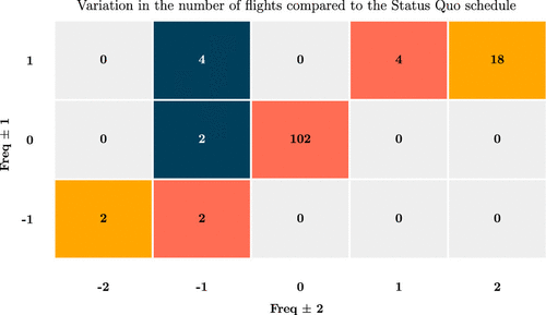
Note. Blue, evaluated with the assumption; orange, evaluated without the assumption.
Figure 5 shows the distribution of the number of flights by flight distance for the YV + YX instance. The left subfigure includes all segments, the middle includes segments with more than one daily flight in the status quo schedule, and the right subfigure includes the segments with more than two daily flights in the status quo schedule. The right subfigure is of particular interest because it shows the trends for only those segments that allow the optimization model to explore the full spectrum of alternatives, ranging from reducing the daily frequency by two to increasing the daily frequency by two. As we move from the “Freq ” schedule to “Freq ” schedule to “Freq ” schedule, we notice that the number of flights increases for most flight distances higher than 400 nm but slightly decreases for the 300- to 400-nm flight distance range. This indicates that a major driver of profit improvement is an increase in longer and more profitable flights with some reduction in the number of shorter-distance flights to satisfy the aircraft utilization constraints. This is consistent with the fact that, as shown in Table 6, compared with the “Freq ” schedule, the average flight distance increases by 2.4% for the “Freq ” schedule and by 2.9% for the “Freq ” schedule.
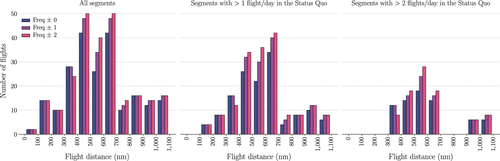
7.3. Value of Comprehensive Schedule Planning
Our approach focuses on a comprehensive timetabling problem, which provides the optimization model complete freedom to choose the departure times and aircraft types for each flight. In comparison, several previous studies have focused on incremental timetabling decisions. The incrementality is manifest in one of two ways: some studies only allow retiming flights within a small window around their departure times in an existing schedule, whereas others only allow choosing flights from a predetermined set of optional flights. Thus, an interesting question relates to the additional benefits accrued by the comprehensive timetabling approach compared with the incremental approaches. Figures 6 and 7 provide one way to visualize these benefits.
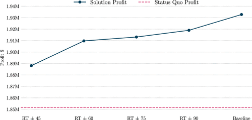
Notes. “Baseline” allows unlimited retiming. “RT ” allows flights to be retimed by minutes compared with the status quo schedule.
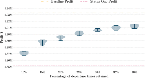
Notes. “Baseline” retains all departure times. Each violin plot uses 10 random draws.
Figure 6 plots the profit of the YV + YX instance against the size of the retiming window. Specifically, from left to right, the window size increases from minutes to minutes. The rightmost point shows the profit for our “Freq ” schedule, which allows unlimited retiming (denoted as “baseline” in this figure). As noted before, the baseline profit is 4.39% higher than that of the status quo schedule. When restricting window sizes to minutes, the profit improvement relative to the status quo schedule decreases to 1.98%. Similarly, window sizes of ±60, ±75, and ±90 minutes yield profit increases of 3.15%, 3.33%, and 3.65%, respectively. Thus, incremental retiming approaches can capture between 45% (for the ±45-minute window size) and 83% (for the ±90-minute window size) of the profit improvement provided by our comprehensive timetabling approach. In other words, we stand to lose more than half of the benefits of our timetable optimization if we restrict departure times to the ±45-minute retiming window.
Our comprehensive timetabling approach decides the periods used as departure times for the flights in each segment, along with the corresponding aircraft type assigned to each selected period. A common way of incremental timetabling in the literature (called the “optional flights” approach) involves preselecting a set of candidate periods in each segment and letting the optimization model choose from those. In essence, this optional flights approach is a restricted version of the comprehensive timetabling that involves fewer periods to choose from. To quantify the additional benefits of comprehensive timetabling compared with the optional flights approach, we characterize the relationship between profit and the number of candidate periods. To this end, we conducted a number of experiments in which we allowed flights to depart only in a subset of the periods in the planning horizon. This subset contains all the departure periods in the status quo schedule, plus other randomly selected periods, totaling z% of the available periods, with . We create 10 random subsets for each value of z and demonstrate the results in Figure 7 as a series of violin plots of the profits against the percentage of candidate departure time periods retained.
Note that we recover approximately half of the benefits of comprehensive timetabling by retaining just 20% of the departure times. However, the profit curve in Figure 7 starts to flatten beyond that point, making it harder to recover the remaining profit gains through this incremental approach. Overall, this figure shows that comprehensive timetabling allows additional profit gains that are between ≈310% (at ) and ≈33% (at ) compared with those achieved by an optional flights approach.
8. Discussion
This paper presented a new column generation–based modeling and algorithmic approach to jointly optimize medium-term schedule planning decisions of a regional airline for a given schedule of the mainline partner carrier. We developed an original mathematical formulation for the integrated optimization of flight timetabling, fleet assignment, frequency planning, and some limited aspects of route planning. Our formulation adopted a composite-variable approach with a very tight continuous relaxation, where each variable indicates a particular segment schedule. Moreover, our formulation endogenously captured passengers’ booking decisions through a sales-based linear programming reformulation of a general attraction discrete choice model. To accelerate column generation, we developed a new strategy using dynamic programming based on a passenger mix model to quickly identify promising columns. Combined with implicit dual stabilization, symmetry breaking, and subproblem aging, this acceleration approach allowed us to solve large-scale real-world instances to near optimality in at most three hours. Further enhancements to the column generation procedure could reduce the runtime even further and are a viable avenue for future research. Extensive computational experiments based on some of the largest real-world regional airline networks that can be constructed using public data sets demonstrated that our approach can yield hundreds of thousands of dollars in daily profit improvements to the airline. In addition, these findings remained stable under a variety of sensitivity and robustness checks.
A promising direction for future research includes extending this modeling and algorithmic framework to airlines that have network structures different from regional airlines. There is also an opportunity to integrate additional modeling considerations related to aircraft routing and crew scheduling into the formulation to enable a more seamless integration with these downstream schedule planning steps. Other practical considerations, such as ground resource availability constraints or the robustness to delays and disruptions, may also be considered in future extensions.
Appendix A. Details of the Master Problem Extensions
This section formalizes the master problem model extensions introduced in Section 4.1.1 using the sets and parameters described in Table A.1.
|
Table A.1. Sets and Parameters Used in Appendix A
| Set | Description |
|---|---|
| Hubs served by the regional airline. | |
| Mainline flights with at least one endpoint at a hub served by the regional airline. | |
| Mainline flights departing from a hub served by the regional airline. | |
| Mainline flights arriving at a hub served by the regional airline. Remark: are hub-to-hub mainline flights. | |
| Mainline flights departing from . | |
| Mainline flights arriving at . | |
| Segments of type for . In words, these are the segments operated by the regional airline with a destination airport that is the origin for a mainline flight . | |
| Segments of type for . In words, these are the segments operated by the regional airline with an origin airport that is the destination of a mainline flight . | |
| Departure times for regional flights on segment such that passengers can then transfer to at . | |
| Departure times for regional flights on segment such that passengers could have transferred from at . | |
| Schedules for segment containing a flight departing in period . | |
| Schedules for segment containing a flight arriving during period . | |
| Schedules for segment containing a regional flight departing during period . | |
| Schedules for segment containing a regional flight departing during period . | |
| Departure periods for regional flights in segment for which parameter (see below) is defined. | |
| Departure periods for regional flights in segment for which parameter (see below) is defined. | |
| Departure periods of flights in schedule . | |
| Arrival periods of flights in schedule . | |
| Departure periods of flights operated with an aircraft of type in schedule . |
| Parameter | Description |
|---|---|
| Maximum number of departures from airport during period . | |
| Maximum number of arrivals at airport during period . | |
| Departure hub for . | |
| Arrival hub for . | |
| Number of passengers on the regional flight from j to departing during period according to schedule , who will later transfer to mainline flight at hub . | |
| Number of passengers on the regional flight from to j departing during period according to schedule , who transferred from mainline flight at hub . | |
| Mainline flight out of taken by passengers of market traveling on a regional flight in segment departing during period . This parameter is only defined for periods t such that a regional-to-mainline transfer is possible at j. | |
| Mainline flight to taken by passengers of market traveling on a regional flight in segment departing during period . This parameter is only defined for periods t such that a mainline-to-regional transfer is possible at i. | |
| Capacity of mainline flight . | |
| Total flight time of an aircraft of type in schedule . | |
| Maximum average flight time for . | |
| Flight time (in periods) from i to j, with on an aircraft of type . |
A.1. Route Selection
Changing the Equality Constraint (1b) to a less-than-or-equal-to constraint changes the domain of the corresponding dual values from to , but does not otherwise affect the column generation procedure.
A.2. Airport Slot Restrictions
We can limit the number of flights departing and arriving at each airport during each period by adding the following two constraints:
The Reduced Cost (2) of a segment schedule is modified by subtracting the following terms:
A.3. Mainline Capacity
We can impose flight capacity constraints on mainline flights by adding the following inequality:
Constraints (A.3) ensure that seating capacities are respected on mainline flights preceding and following the connecting regional flights. The first sum counts regional passengers arriving at the departure hub of mainline flight g and then transferring to g. The second term counts regional passengers arriving at the arrival hub of mainline flight g and then transferring to a regional flight. The reduced cost of a segment schedule is modified by subtracting term
A.4. Aircraft Utilization
We impose maximum average utilization constraints using the following inequalities.
The sum on the right-hand side counts how many aircraft of type a are used in the solution. This number typically equals the fleet size because airlines use all the available aircraft. The reduced cost of a schedule is changed by subtracting the following term.
Appendix B. Case Study Setup
We test our modeling and computational approach on instances based on real-world data on the U.S. domestic market gathered from multiple data sources, namely, the Airline On-Time Performance (AOTP) data set, the Airline Origin and Destination Survey (DB1B), and the Form 41 data set from the Bureau of Transportation Statistics (2023a, b, c) and the aircraft registration database from the Federal Aviation Administration (2023). We used data from June 2022 and considered United Airlines (UA) as the mainline carrier and Mesa Airlines (YV), Republic Airways (YX), and SkyWest Airlines (OO) as regional airlines. This choice is motivated by the greater data availability, partly because of data reporting obligations for airlines above a certain size compared with alternatives. We consider both the optimization of each regional airline by itself and jointly. In the latter case, our instance uses 7 hubs (ORD, EWR, IAD, IAH, LAX, SFO, and DEN) and 149 spokes for a total of 534 nonstop segments and 3,312 markets (see Figure B.1). Figure B.1 depicts the geographical distribution of hubs and spokes included in the instances. It shows that our instances cover almost all parts of the continental United States. We now describe how to estimate the main model parameters from the above data sources.
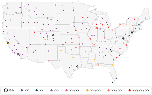
B.1. Fleet Composition, Costs, Fares and Market Sizes
We use our data sources to determine how many aircraft each regional airline employs to operate flights ticketed under United Airlines’ United Express brand. In addition to collaborating with United Airlines, Mesa also operated under the American Airlines’ American Eagle brand until 2023, Republic operates under the American Eagle and Delta’s Delta Connection brands, and SkyWest operates under the Alaska Airlines, American Eagle, and Delta Connection brands. The aircraft registration database and the airline company websites report the aircraft capacities. We estimate operating costs using the short-haul formulas of Swan and Adler (2006), adjusted for inflation. We use fares data from the DB1B database. For multileg itineraries, only the total fare is available; in this case, we assume that the regional leg fare is proportional to its length. We derive flight times and minimum turnaround times from AOTP data; in particular, we have minimum turnaround times that are functions of both the aircraft type and the airport. Note that, as is the typical case for regional airlines, there are only a small number of distinct aircraft types across the entire fleet of our case study networks of regional airlines. They consist primarily of Canadair regional jets (CRJs) and Embraer aircraft. We generate our data on market sizes and reasonable paths through the network using the DB1B database. Because DB1B includes a 10% sample of passenger tickets, we scaled it up by multiplying by 10, and then by a further factor of 1.1 to account for passengers who used the outside option in order to obtain the total market sizes.
B.2. Attractiveness Data
We compute attractiveness values using the method proposed by Barnhart, Fearing, and Vaze (2014) and assuming a minimum connection time of 30 minutes for one-stop itineraries. To do this, we used the mainline schedules of a reference day, June 29, 2022. The attractiveness is given by the following formula:
Following the state-of-the-art literature on choice-based airline schedule planning (e.g., Wei, Vaze, and Jacquillat 2020; Yan, Barnhart, and Vaze 2022), we set the shadow attractiveness value to zero. Therefore, our adjusted attractiveness is equal to the attractiveness . Airline industry practitioners, who have access to vast amounts of passenger booking and transactions data sets, could use such internal data to statistically estimate shadow attractiveness and adjust accordingly. Appendix G evaluates the impact of other values of shadow attractiveness on the performance of our solutions.
Given the market sizes, the attractiveness values , and the number of passengers carried from our data sources, if the flights were not subject to seating capacities, we could apply Equation (6) to recover the attractiveness values of the outside option . However, because of the seating capacity limits, the ratio between the number of passengers taking each option (including the outside option) does not necessarily match the ratio between the options’ attractiveness values. Therefore, we use the following approach to derive realistic values of . First, we produce estimates , disregarding seating capacities. Note that if these estimates were correct, solving Problems (7a)–(7h) with the fixed real-world schedule would give passenger numbers that closely match those observed in the data. Otherwise, we should adjust the values of to make the numbers match. However, each can potentially require a different adjustment factor, making the search for such factors computationally expensive and prone to overfitting to the data. To overcome this issue, we adjust all estimates simultaneously using a single multiplicative factor from a small search grid (15 logarithmically distributed values between and one, in our case). To select the best factor, we quantify the similarity between the passenger numbers obtained from (7a)–(7h) and the real ones using their mean absolute deviation.
Appendix C. Key Computational Statistics
Table C.1 details the time used and the columns generated by our proposed approach in its base configuration. We report on the same seven instances used in Table 4. The time breakdown reports the percentage time used by Gurobi when solving the linear relaxation of the restricted master problem (column “MP-LP”), the pricing subproblem solved by the DP algorithm of Section 5.2 (column “SP-DP”), the pricing subproblem solved directly by Gurobi (column “SP-MIP”), and Gurobi when solving the restricted master problem as an MIP with the generated segment schedules (column “MP-MIP”). Recall that we solve the pricing subproblem as an MIP if the DP procedure returns an infeasible column or a feasible column with a positive approximate relaxed reduced cost (RRC), whose actual reduced cost is nonpositive. “Tot” lists the number of columns generated by solving the pricing subproblem and used in the final MIP. It refers only to the variables and does not include the variables. This total is further decomposed into columns generated by the DP algorithm (“SP-DP”) and by the MIP pricing subproblem formulation (“SP-MIP”).
|
Table C.1. Detailed Breakdown of the Time Used by the Proposed Column Generation Approach, and the Number of Columns Generated
| Time | Columns | ||||||
|---|---|---|---|---|---|---|---|
| Instance | MP-LP% | SP-DP% | SP-MIP% | MP-MIP% | Total | SP-DP% | SP-MIP% |
| YV | 6.5 | 24.2 | 69.3 | 0.0 | 417 | 64.9 | 35.1 |
| YX | 1.4 | 26.1 | 72.6 | 0.1 | 460 | 67.1 | 32.9 |
| OO | 4.9 | 20.1 | 74.7 | 0.3 | 2,053 | 65.4 | 34.6 |
| YV + YX | 3.6 | 26.3 | 69.9 | 0.2 | 1,460 | 64.5 | 35.5 |
| YV + OO | 1.9 | 21.9 | 76.0 | 0.2 | 2,999 | 63.9 | 36.1 |
| YX + OO | 7.1 | 24.3 | 68.1 | 0.5 | 2,515 | 63.4 | 36.6 |
| YV + YX + OO | 1.2 | 21.4 | 77.3 | 0.1 | 3,481 | 63.3 | 36.7 |
Table C.1 shows that the vast majority of the time is spent solving the pricing subproblems. Repeatedly solving the linear relaxation of the master problem takes between 1.2% and 7.1%, whereas the final MIP only uses a tiny fraction of the time, never exceeding 0.5%. The DP algorithm generates around two-thirds of the columns using around a quarter of the total time spent solving the subproblems (). The MIP formulation uses three-quarters of the time spent solving the subproblems to produce the remaining one-third of the columns and to certify that no positive-reduced-cost column exists. Importantly, though, this time can be explained more by the large number of MIPs solved, rather than the general difficulty of Formulation (7a)–(7h). The number of MIPs solved depends on the instance sizes (with up to 534 segments, i.e., up to 534 subproblems (7a)–(7h) to solve at each iteration, for the largest instance YV+YX+OO) and on the number of column generation iterations, which ranged from 201 for the YV instance to 6,122 for the YV + OO instance. On the other hand, solving a single pricing subproblem MIP is extremely fast. For example, for the YV + YX instance, the mean time spent to solve one pricing subproblem MIP is 0.035 seconds (median: 0.008 seconds), and the mean number of branch-and-bound nodes explored by Gurobi is 173 (median: one, 85th percentile: one).
Appendix D. Early Termination
To use our algorithm for faster decision making or to perform multiple scenario analyses on large instances, we might want to reduce its computational runtime by terminating the column generation procedure early. We would then obtain a primal solution via the reduced master heuristic. Unfortunately, we would not have a valid dual bound to assess the solution’s quality because we did not solve [MP] to optimality. In the following, we derive a Lagrangian bound (see, e.g., Lübbecke and Desrosiers 2005) that is valid even in case of early termination. Let be the unknown optimal objective value of [MP] and be the optimal objective value of an instance of the reduced [MP]. Let be the highest reduced cost of a column of , according to the duals of the reduced [MP]. We can obtain by solving all pricing subproblems to optimality. We then choose, for each subproblem, the generated column with the highest reduced cost, if positive. Otherwise, if a subproblem for proves that no positive reduced cost column exists, . We can then use a Lagrangian bound to obtain that , where Constraints (1b) act as convexity constraints on each set (see, e.g., Wolsey 2021, section 11.5.1).
Appendix E. Regional-Mainline Mixed Segments
All results in the main body of the paper assumed that each segment is operated exclusively by a regional airline or exclusively by a mainline carrier. This is true for almost all segments in our real-world airline data sets. Specifically, in the YV+YX instance, 64 of the 67 hub-to-spoke (and, correspondingly, 64 of the 67 spoke-to-hub) segments are operated exclusively by regional airline flights. In the remaining three hub-to-spoke (and three spoke-to-hub) segments, there was at least one daily flight operated by a mainline aircraft and at least one operated by a regional aircraft. In the YV+YX instance, the mainline aircraft operate at least one daily flight on the IAH-DFW, EWR-CLE, and EWR-RDU hub-to-spoke segments and on their three symmetric spoke-to-hub counterparts. Specifically, in the reference day used for our experiments, June 29, 2022, there were two mainline flights on each of these six segments. Interestingly, these 12 flights were operated with 12 different aircraft, which were also used on other mainline segments that are not part of the regional network. The aircraft types used were Boeing 737, Airbus A319, and Airbus A320.
In our passenger allocation model used to generate the results in the main body of the paper, we account for all passengers in each market and allocate them to all itineraries regardless of whether the flights in that itinerary are operated by the regional or the mainline. However, our optimization model optimizes the scheduling decisions of only regional flights while assuming that the mainline flights remain fixed. In reality, mainline and regional airlines can schedule flights on the hub-to-spoke and spoke-to-hub segments at some level of coordination to ensure that overall profits are maximized. Indeed, our model can include these mainline flights and, if appropriate, can even perform limited destination selection or retiming of mainline flights. In the following, we present two ways in which this coordination can be incorporated into the model presented in Section 4, along with the results of the corresponding experiments.
In both experiments, we enlarge the set A of aircraft types to include the mainline aircraft, and we force the model to deploy the same number of mainline aircraft as were used on regional segments in real life (that is, 12 aircraft). In the first experiment, we allow these aircraft to be used only on those segments and at those times that are compatible with their remaining schedule on the rest of the network. We incorporate these restrictions by appropriately fixing some of the variables in the master problem and some of the variables in the subproblems (for the aircraft types corresponding to mainline aircraft). Although this means that we significantly constrain the mainline aircraft’s availability because of the requirement to be able to use them on the rest of the network for certain parts of the day, we now include the mainline aircraft in both the master problem and the pricing subproblem. The model then optimizes the schedule on all regional and mixed segments while including these mainline aircraft. We refer to this scenario as the “fixed segments” scenario.
In the “free segments” scenario, conversely, we do not constrain the segments on which the mainline aircraft can be used, nor the times of day when they can operate. We still require that they are used on the regional segments for up to the same amount of time as in real life (i.e., they cannot become “full-time” regional aircraft). In this case, we assume that the mainline will appropriately change its timetable to be compatible with the mainline flights on the regional segments.
Table E.1 reports the results of this experiment. The upper part of the table refers to the revenue, cost, and profit obtained by the regional airlines when not explicitly including flights operated by the mainline; therefore, it reports the same results as Table 5. The bottom part includes mainline flights and reports the overall revenue, cost, and profit obtained by the regional airlines and the mainline in the “fixed segments” and “free segments” scenarios. It is important to note that all results in Table E.1 are obtained for the same set of 134 (hub-to-spoke and spoke-to-hub) segments.
|
Table E.1. Results on the YV+YX Instance, Considering Only the Regional Airlines’ Fleet and Also Including Some Mainline Aircraft in the “Fixed Segments” and “Free Segments” Scenarios Described in Appendix E
| Revenue | Cost | Profit | IAH DFW | EWR CLE | EWR RDU | EWR ORF | EWR BUF | IAD RDU | ||
|---|---|---|---|---|---|---|---|---|---|---|
| Regional only | Status quo | 3,387,407 | 1,535,941 | 1,851,465 | ||||||
| Freq | 3,471,732 | 1,538,942 | 1,932,790 | |||||||
| (+2.49%) | (+0.20%) | (+4.39%) | ||||||||
| Regional and mainline | Status quo | 3,769,105 | 1,608,283 | 2,160,822 | 2 | 2 | 2 | 0 | 0 | 0 |
| Freq fixed segment | 3,873,509 | 1,611,338 | 2,262,171 | 2 | 2 | 2 | 0 | 0 | 0 | |
| (+2.77%) | (+0.19%) | (+4.69%) | ||||||||
| Freq free segment | 3,915,574 | 1,610,588 | 2,304,986 | 2 | 1 | 0 | 1 | 1 | 1 | |
| (+3.89%) | (+0.14%) | (+6.67%) |
When accounting for mainline flights on regional segments, the status quo revenue is higher, with more seats flown but only higher cost. Consequently, accounting for mainline flights on regional segments corresponds to more profit in the status quo solution.
When comparing optimized solutions with the corresponding status quo, we note that the optimal “fixed segments” solution has a slightly higher profit increase () than that of the optimal solution that only includes regional aircraft (). In the “free segments” scenario, the profit increases even further (), and the difference from the status quo is considerably greater than the one we obtain when including only regional aircraft ().
In the “free segments” scenario, we obtain a higher revenue by deploying the larger mainline aircraft partially on different segments compared with those of the status quo solution. Although the solution maintains two flights per day in each direction on the IAH DFW segment pair, it reduces the number of daily flights on the EWR CLE segment pair to one in each direction and on the EWR RDU segment pair to zero. The model redeploys the corresponding aircraft on three other segment pairs. One is IAD RDU, which confirms the importance of RDU, but prefers to serve it with a larger aircraft from the IAD hub. The others are EWR ORF and EWR BUF, which involve shorter flights that can feasibly replace the flights on EWR CLE and EWR RDU segment pairs.
In summary, the experiments in this appendix handle mixed segments involving both regional and mainline aircraft as part of the overall optimization problem and demonstrate significant incremental benefits in terms of revenue and profit increases. Specifically, we observe that when handling mixed segments as part of the optimization, we generate of additional revenue increase and of additional profit increase per mixed segment exclusively through retiming. Furthermore, the numbers increase to in additional revenue increase and in additional profit increase when we additionally allow limited swapping of aircraft between mixed and regional-only segments.
Appendix F. Impacts of Demand Uncertainty and Revenue Management Practices
The results presented in Section 7 have assumed that the demand for each passenger itinerary is deterministic and that the average fares for each itinerary are known and fixed. In practice, passenger demand can fluctuate considerably from one day to another, and this uncertainty can impact the actual number of passengers carried by the airline. Too few passengers on a given day can lead to reduced revenue, whereas too many passengers compared with those estimated can lead to some passengers not being accommodated (or getting “spilled”) because of aircraft seating capacity limits. Spill estimation models usually make some assumptions about the demand distribution and compute the expected number of passengers as the expected value of the demand distribution truncated by the number of seats. As mentioned in Section 7, our results have indirectly captured the effects of demand uncertainty by imposing a hard upper limit of 93% on the maximum number of seats sold in each segment.
The load factor is a nondecreasing function of the demand factor. The demand factor is the ratio of passenger demand divided by seat capacity. All else being equal, adding more flights to a segment, thus increasing the seat capacity, would decrease the demand factor. Our “Freq ” and “Freq ” schedules have more segments with an increase rather than a decrease in flight frequency and number of seats per segment. This implies that we should expect a slightly lower demand factor. Of course, by offering flights at desirable departure times, we hope to attract more passenger demand, thus increasing the numerator of the demand factor. Our results in Section 7.1 simplify these complexities using a hard upper limit on load factors.
In addition, nearly all airlines practice revenue management (RM) methods, which greatly affect the fares of spilled passengers because they try to ensure that spilled passengers are predominantly low-fare passengers in a given segment. Our results in Section 7.1 simplify this effect by assuming identical fares for all passengers in a given market. Belobaba and Farkas (1999) showed that revenue management practices affect spilled passenger fares and the number of spilled passengers. In this section, we use the approach proposed by Belobaba and Farkas (1999) to approximately capture the effects of demand uncertainty and revenue management practices on the number of passengers carried, the average fares of the passengers carried, and, consequently, the profit of the airline. Similar to the process described in Vaze and Barnhart (2012, section 5.4), we change the fare of each market in each segment by applying the correction suggested by Belobaba and Farkas (1999). This results in a new instance with different values of the fare parameters . We then reoptimize this instance by running our column generation algorithm again without imposing any hard limit on the load factors, thus obtaining a new schedule informed by the new corrected fares and the corresponding changes in passenger demand. However, the new optimized schedule adds and removes flights (and thus changes seat capacity) in some or all segments. This, in turn, introduces a feedback effect because it alters the extent of the fare correction. Therefore, we propose an iterative procedure in which a correction phase and a reoptimization phase alternate until convergence. In our case, two iterations are enough to converge to stable fare values.
Table F.1 presents the key financial performance metrics of the solutions obtained for the joint network instance (YV + YX) by our approach without (second to fourth column) and with (fifth to seventh column) the aforementioned iterative correction and optimization (ICO) process. In addition, Table F.2 presents the key operational metrics for the same instance without (third to fifth column) and with (sixth to eighth column) the ICO process. First, as expected, the operational and financial performances of the “Freq” instances with and without the ICO process are quite similar to each other. However, in the “Freq” and “Freq” instances, the ICO process leads to fewer and shorter flights with slightly higher RASM and CASM values, slightly fewer passengers, and similar average fares, leading to slightly lower profits. Nevertheless, across all three scenarios (“Freq,” “Freq,” and “Freq”), we continue to see a significant profit increase of between 3.68% and 8.84% relative to the status quo solutions. This shows the relative stability of the overall improvements generated by our approach under the effects of demand uncertainty and RM practices.
|
Table F.1. Comparison of the Key Financial Metrics of the Solutions of the Joint Network Instance (YV + YX) with and Without Applying the ICO Process Described in Appendix F
| Without correction | With correction | |||||
|---|---|---|---|---|---|---|
| Revenue | Cost | Profit | Revenue | Cost | Profit | |
| Status quo | 3,387,407 | 1,535,941 | 1,851,465 | 3,387,407 | 1,535,941 | 1,851,465 |
| Freq | 3,471,732 | 1,538,942 | 1,932,790 | 3,458,547 | 1,538,942 | 1,919,605 |
| (+2.49%) | (+0.20%) | (+4.39%) | (+2.10%) | (+0.20%) | (+3.68%) | |
| Freq | 3,713,894 | 1,670,419 | 2,043,474 | 3,589,626 | 1,589,970 | 1,999,656 |
| (+9.64%) | (+8.76%) | (+10.37%) | (+5.97%) | (+3.52%) | (+8.00%) | |
| Freq | 3,790,470 | 1,692,362 | 2,098,108 | 3,637,440 | 1,622,231 | 2,015,209 |
| (+11.90%) | (+10.18%) | (+13.32%) | (+7.38%) | (+5.62%) | (+8.84%) | |
|
Table F.2. Comparison of the Key Operational Metrics of the Solutions of the Joint Network Instance (YV + YX) With and Without Applying the ICO Process Described in Appendix F
| Without correction | With correction | ||||||
|---|---|---|---|---|---|---|---|
| Status quo | Freq | Freq | Freq | Freq | Freq | Freq | |
| Number of flights | 218 | 218 | 240 | 246 | 218 | 228 | 236 |
| Average flight distance | 571.0 | 571.0 | 584.7 | 587.4 | 571.0 | 579.2 | 581.1 |
| RASM | 36.5 | 37.3 | 35.5 | 35.2 | 37.3 | 36.0 | 35.8 |
| CASM | 16.6 | 16.5 | 16.0 | 15.7 | 16.6 | 16.2 | 15.9 |
| Passengers carried | 14,908 | 14,920 | 16,211 | 16,666 | 14,922 | 15,676 | 16,151 |
| Nonstop | 66% | 66% | 66% | 66% | 66% | 66% | 66% |
| One stop | 34% | 34% | 34% | 34% | 34% | 34% | 34% |
| Average fare | $227 | $233 | $229 | $227 | $231 | $229 | $227 |
| Nonstop | $223 | $229 | $227 | $225 | $228 | $227 | $225 |
| One stop | $242 | $246 | $238 | $236 | $244 | $240 | $238 |
| Light retiming | — | 63% | 58% | 60% | 65% | 61% | 60% |
Appendix G. Impact of the Different Values of Shadow Attractiveness on the Profits
In this appendix, we evaluate the impact of using nonzero values of shadow attractiveness on the profitability of our solutions. Specifically, we set the shadow attractiveness value () of taking a flight from i to j in period t for a passenger of market q as a fraction of the attractiveness . In other words, we set . Figure G.1 shows the profit obtained by sampling the values of uniformly from [0%, 5%] and also from [0%, 10%] and then rerunning our solution approach on the VY+YX instance. We repeat each experiment 10 times and present the resulting violin plots of the optimized profit. As shown in the figure, the nonzero shadow attractiveness values lead to a small reduction in profits of the order of 0.46% and 0.31% on average for the two experiments with [0%, 5%] and [0%, 10%] sampling, respectively. Nevertheless, across the 20 runs of these two experiments, we note that the overall profit improvement always stays above 3.1% compared with the status quo. This shows that regardless of the exact values of the shadow attractiveness, our approach continues to produce a consistent and robust profit improvement in all the experimental scenarios that we tested.
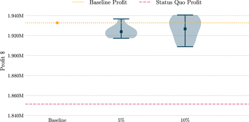
Appendix H. Independent Evaluation of Profit Using a Passenger Booking Simulator
A limitation of the results presented in Section 7 is that they are based on a passenger allocation model relying on the SBLP approach. This approach does not account for the passengers’ booking arrival process, the associated uncertainty, the impact of multiple booking classes per itinerary, and the effects of revenue management practices. In this appendix, we present an independent and more accurate evaluation of the profit improvement achieved by our optimized FTFA schedules, which overcomes these limitations. To do so, we use a detailed passenger booking simulator based on the one introduced by Yan, Barnhart, and Vaze (2022).
Different from the approach presented in Section 4, our simulator considers both the regional and mainline networks. This includes mainline and regional segments, markets served by the regionals only, markets served by regionals and the mainline, and (unlike the approach in Section 4) markets served by the mainline only. In this way, the simulator explicitly accounts for the mainline flights’ capacity, rather than relying on the notion that there is a fixed number of seats on mainline flights that are reserved for regional passengers, as initially proposed in Section 4.1.1. Therefore, the passenger mix (nonstop versus connecting) in each mainline flight is determined endogenously by the simulator itself.
Our simulator divides the booking horizon into booking periods. This roughly corresponds to a six-month horizon divided into weekly booking periods. This is consistent with industry practice in which the booking horizon is often several months long and is split into several booking periods. The number of passengers of a market arriving in each booking period follows a Poisson distribution with rate . Upon arrival, each passenger selects a fare product out of a set of available fare products with probability
In our simulator, at the beginning of each booking period, the airline decides which fare products to offer in that booking period. This decision is made based on the remaining seat availability throughout the airline network and the distribution of the remaining demand forecast. It is important to note that our approach assumes knowledge of the distribution of the remaining forecast demand, but not its actual realization, which is consistent with what happens in reality. Our simulator uses a typical bid price control approach for network-wide revenue management. Bid prices are calculated based on the dual variables of market size and capacity constraints of a network-wide passenger allocation formulation. This formulation is analogous to Formulation (J.1a)–(J.1f) in Appendix J.1; thus, market size and capacity constraints are analogous to (J.1c) and (J.1d), respectively. However, whereas the Formulation (J.1a)–(J.1f) only includes regional segments and markets, the allocation model used in the simulator includes both mainline and regional segments and markets. According to the standard industry practice in bid price control, a fare product is offered if and only if the fare is at least equal to the sum of the dual prices. The passenger allocation model is resolved—and, therefore, the duals are recomputed—at each booking period, with updated values for the network-wide seat availability and the remaining demand forecast. The reader is referred to Gallego and Topaloglu (2019) and Yan, Barnhart, and Vaze (2022) for additional technical details on this bid price control approach.
The first row of Table H.1 shows, for the optimized YV+YX FTFA schedule, the profit increase estimated with the passenger allocation model based on the SBLP and the profit increase estimated using the simulator. In each case, the profit increase is the difference between the profit in the optimized FTFA schedule and the profit in the status quo solution. Furthermore, our simulator models passenger booking as a Poisson process with a given arrival rate and thus accounts for uncertainty in the passenger demand arrival process. As a consequence, the simulator results are affected by demand stochasticity. The first number in the “simulation profit increase” column of the table reports the average profit increase over 100 simulator runs, followed by its 95% confidence intervals. Note that in the table, all values are reported as a percentage of the corresponding average status quo solution profit for ease of comparison.
|
Table H.1. Profit Comparison of the Optimized FTFA Schedules Computed According to the PAM Based on the SBLP and a Passenger Booking Simulator
| Perturbation | Scenario | SBLP-based PAM profit increase (%) | Simulation profit increase (%) | |
|---|---|---|---|---|
| No | — | 4.39 | 4.10 | |
| ±5% | 1 | 3.35 | 3.94 | |
| 2 | 3.37 | 3.28 | ||
| 3 | 3.47 | 3.51 | ||
| 4 | 3.45 | 3.62 | ||
| 5 | 3.45 | 3.67 | ||
| ±10% | 1 | 1.67 | 3.34 | |
| 2 | 1.56 | 2.79 | ||
| 3 | 2.13 | 3.48 | ||
| 4 | 2.29 | 3.21 | ||
| 5 | 1.58 | 3.56 | ||
| ±15% | 1 | 0.38 | 1.77 | |
| 2 | 0.40 | 2.34 | ||
| 3 | 0.40 | 2.34 | ||
| 4 | 0.43 | 3.14 | ||
| 5 | 0.22 | 1.91 | ||
Additionally, the passenger arrival rate used in the simulator, which corresponds to the forecast average demand in any booking period, may contain errors because of inaccurate estimates of the attractiveness of each product and/or the outside option. To account for this additional source of uncertainty, we evaluate profits under imperfect estimates of attractiveness values. In particular, we generate scenarios in which all attractiveness values are perturbed through a uniformly random variation of up to ±5%, ±10%, and ±15%. We generate five scenarios for each of these three perturbation levels. In each scenario, we construct a new flight schedule by resolving the FTFA model with the algorithm presented in Section 5 using the perturbed attractiveness values. The resulting schedule represents the one obtained under imperfect demand assumptions. The corresponding SBLP-based and simulation profit increase estimates are presented in rows 2–16 of Table H.1. In other words, these results in the last 15 rows of Table H.1 are obtained under the assumption of knowledge of an erroneous distribution of the remaining demand.
The first row of Table H.1 shows that the average profit increase estimated by the booking simulator (4.10%) is comparable to that calculated by the SBLP-based PAM (4.39%). Moreover, the corresponding 95% confidence interval shows that even the lower bound of this interval is only 0.44 percentage points lower than the SBLP-based profit estimate. This independent objective evaluation of the optimized FTFA schedules highlights the stability of the superior performance of our optimized schedules. Moreover, the fact that the profit estimates remain highly stable throughout the 100 simulation runs with varying demand samples in each booking period demonstrates the robustness of the FTFA performance under the uncertainty in passenger demand. As mentioned in Section 7, our optimization model indirectly captured the effects of demand uncertainty by imposing a hard upper limit of 93% on the maximum number of seats sold on each segment. We found that in the optimal solution, when evaluated under the SBLP-based PAM, only 16 of the 218 flights had a 100% load factor, whereas 75 of the 134 segments had an average load factor reaching the 93% upper limit. Moreover, for the same optimal solution, when evaluated under our passenger booking simulator, only 13 of the 218 flights had a 100% load factor, whereas 61 of the 134 segments had an average load factor at or above 93%. This further demonstrates the consistency between the results obtained via both evaluation approaches.
The remaining 15 rows of the table lead to several interesting observations. First, we note that, based on both the SBLP-based PAM and the simulator, the profit gains achieved by our FTFA schedules deteriorate to some extent with increasing levels of forecast errors. This is not surprising. The second and perhaps more interesting observation is that this deterioration is less for the simulator-based evaluation than for the SBLP-based PAM evaluation. This demonstrates the benefits of the iterative revenue management control policy used throughout the booking horizon. As described above, the simulator implements an intelligent control of itinerary product availability across the network by adapting to the realized demand and leftover capacity in each booking period. This ensures that the damage from schedules optimized based on incorrect data is partly mitigated and results in a smaller deterioration in profit. Finally, the biggest takeaway from the last column of Table H.1 is that a conservative estimate of the profit increase achieved by our FTFA schedules relative to the status quo solutions never drops below 1.64%. This conservative estimate refers to the smallest value of the lower bound in the two-sided 95% confidence intervals across 100 simulation runs for each of the five scenarios at each of the three perturbation levels tested in our experiments.
In summary, this independent objective evaluation of our FTFA schedules underscores their consistently superior performance across the various assumptions related to the stochastic passenger booking arrival process, forecast errors in product attractiveness values, the impact of multiple booking classes per itinerary, and the effects of revenue management practices.
Appendix I. Impact of Connection Times
Recall our assumption that all passengers in the same market follow the same itinerary if their itinerary includes one regional flight and one mainline flight, and they take the same regional flight. For example, all passengers on the MAF-IAH-ORD path, who take a regional MAF-IAH flight with Mesa Airlines that departs at 08:00 and arrives at 10:00, will continue their itinerary on the same mainline flight. If there are mainline flights departing at 10:50, 11:50, and 12:50 on segment IAH-ORD, then all MAF-IAH-ORD passengers arriving on the Mesa flight to IAH at 10:00 will take the 10:50 departure to ORD, assuming that the 50-minute connection time is more desirable for passengers than the 110- or 170-minute connection times. Specifically, we assume that all passengers will choose the connection with the shortest connection time above a minimum value of 30 minutes. In this section, we evaluate the impact of relaxing this assumption by allowing passengers on the same path and the same regional flight to choose from multiple mainline flights. Specifically, Figure I.1 shows the effect of a varying percentage of passengers choosing a connection with 30 versus 60 minutes of minimum connection time. Figure I.1 demonstrates that minor violations of our assumption (for example, changing the percentage of passengers with a 30-minute minimum connection time from 100% to 80% or 90%) result in only slight changes in total profit (by 0.12%–0.36%). However, larger violations (for example, changing the percentage from 100% to 50%, 60%, or 70%) can dilute the profit improvements generated by our approach. This emphasizes that in order to maximize the benefits of our approach, it is critical to capture passenger preferences with at least a moderate level of accuracy.
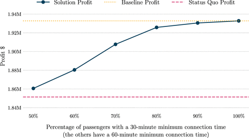
Appendix J. Sensitivity to the Regional-Regional Split Market Assumption
Recall that we split markets that are served with an itinerary composed of two regional flights (spoke A–hub–spoke B) into two separate markets (spoke A–hub and hub–spoke B). These passengers represent a small fraction of the total market size (see Table 1). For example, as mentioned in Section 3, when considering mainline UA and regionals YV and YX, only 1.33% of the passengers use an itinerary with more than one segment operated by regional airlines. This introduces some inaccuracy in our final results. However, the direction and magnitude of this inaccuracy are unclear because this assumption causes two opposite effects.
On the one hand, rescheduling some regional flights might break a previously feasible connection at the hub. Under the split market assumption, we still optimistically allocate passengers affected by this disruption to our spoke A–hub and hub–spoke B flights. In reality, these passengers might not be able to complete their itinerary using the new schedule. On the other hand, the new schedule might now enable new connections that were not possible in the status quo schedule, creating new markets that were previously not served. The first effect suggests that our results presented in Section 7.1 might overestimate the true profit improvement, whereas the second effect suggests that they might underestimate it.
In this section, we estimate the net impact of these two opposite effects by focusing on the YV + YX instance. We first solve the three scenarios (“Freq,” “Freq,” and “Freq”) using our column generation algorithm while retaining the split market assumption. Then, we fix the resulting schedules and replace the split markets (spoke A–hub and hub–spoke B) with the original spoke A–hub–spoke B markets. At the same time, we introduce new markets not present in the original instance because they were currently unserved, and therefore, their passengers did not appear in the databases we used. For this reason, we do not know the exact market sizes and fares for these new markets. We estimate the sizes of the new markets using a gravity model (see, e.g., Morley, Rosselló, and Santana-Gallego 2014) and estimate their fares by choosing, for each new market, the existing market with the most similar size and assuming the same fare per mile. In this way, we avoid using the fare of a large market for a small one, and vice versa. Finally, we run a network-wide passenger allocation model (described in Appendix J.1) using these market sizes and attractiveness values calculated using the estimated fares for the possible itineraries in the new schedule.
Figure J.1 shows the resulting profits with (in blue) and without (in orange) the split market assumption. We find that the net impact of these two opposite effects can be positive or negative. In case of the “Freq” and “Freq” instances, relaxing the assumption leads to a slight reduction in the profit improvement (between 1.3 and 1.6 percentage points) obtained by the optimized schedules, whereas the “Freq” instance shows a higher profit improvement (by 2.7 percentage points) when we relax the assumption. In fact, the average profit for the three instances remains almost identical (within ) with and without the split market assumption.
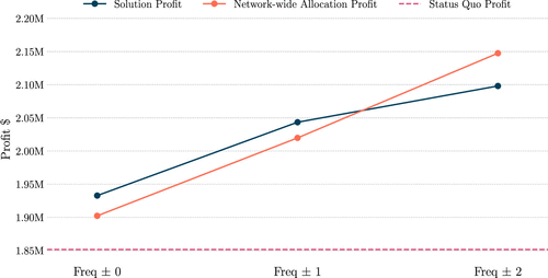
J.1. Passenger Allocation Model for Relaxing the Regional-Regional Split Market Assumption
In the following, we present the approach used to allocate passengers to the optimized schedule under the split market assumption when new markets are introduced. Recall that Q denotes the set of all markets (sets and parameters used in this appendix are defined in Table J.1). We retain the symbols used in the main body of the paper ( and for the attractiveness of all itineraries and the outside option, for the fare, for the market size), but we give them different indices and slightly different meanings, as explained in Table J.1. We now solve a network-wide passenger allocation model for the entire network rather than solving a segment-by-segment pricing subproblem as in Section 4.2; therefore, we update the meaning of the above parameters to reflect this change. Similarly, we continue to use the letter x for the following variables. The variable for denotes the number of passengers in market q who choose the outside option. The variable for and denotes the number of passengers in market q who start their itinerary at time t and use one or more regional flights. We note that the passenger’s itinerary can start with a regional flight (eventually followed by a mainline or another regional flight) or with a mainline flight (followed by a regional one). Indeed, we include in our model the following itinerary types: (a) regional, (b) regional + mainline, (c) mainline + regional, and (d) regional + regional. Whereas our optimization model included itineraries of types (a)–(c), we also include itineraries of type (d) in the following passenger allocation model.
|
Table J.1. Sets and Parameters Used in Appendix J.1
| Set | Description | |
|---|---|---|
| Q | Set of all markets, including the new ones created when the split market assumption is relaxed. | |
| Itinerary start periods for passengers. It is a superset of T because an itinerary could start before our planning horizon. | ||
| Departure times of flights on segment in the optimized schedule. | ||
| Set of tuples of the form describing regional flights with flight origin i, flight destination j, flight departure time s, and aircraft type a, which are used by passengers in market starting their itinerary at time . Because we include both nonstop and one-stop passengers, its size can be zero, one, or two. | ||
| Parameter | Description | |
| Binary parameter taking value one if there is a flight on segment operated by an aircraft of type at time in the optimized schedule. | ||
| Aircraft type used to operate a flight on segment at time in the optimized schedule. | ||
| Fare for a passenger in market starting their itinerary at time flying on the segment(s) operated by the regional airline. Unlike in Section 4, an itinerary in this passenger allocation model can include flights in two regional airline segments. | ||
| Attractiveness of the itinerary that starts at time in market . | ||
| Adjusted attractiveness of the itinerary that starts at time in market . | ||
| Attractiveness of the outside option for market . | ||
| Adjusted attractiveness of the outside option for market . | ||
| Size of market . | ||
Note. A “” next to the parameter name indicates that this parameter has been redefined with a related but slightly different meaning than in Section 4.
A linear programming formulation for the network-wide passenger allocation model reads as follows.
The Objective Function (J.1a) maximizes the fare revenue. Constraints (J.1b), (J.1c), and (J.1d) are analogous, respectively, to (7c), (7d), and (7e), but now adapted to the network-wide passenger allocation model. We note that market sizes for new markets were estimated according to the formula
References
- (1989) Applying integer linear programming to the fleet assignment problem. Interfaces 19(4):20–28.Link, Google Scholar
- (2017) Airline flight schedule planning under competition. Comput. Oper. Res. 87:20–39.Crossref, Google Scholar
- (2007) A very large-scale neighborhood search algorithm for the combined through-fleet-assignment model. INFORMS J. Comput. 19(3):416–428.Link, Google Scholar
- (2019) A robust pairing model for airline crew scheduling. Transportation Sci. 53(6):1751–1771.Link, Google Scholar
- (2009) Airline fleet assignment with enhanced revenue modeling. Oper. Res. 57(1):231–244.Link, Google Scholar
- (2014) Modeling passenger travel and delays in the national air transportation system. Oper. Res. 62(3):580–601.Link, Google Scholar
- (2002) Itinerary-based airline fleet assignment. Transportation Sci. 36(2):199–217.Link, Google Scholar
- (1999) Yield management impacts on airline spill estimation. Transportation Sci. 33(2):217–232.Link, Google Scholar
- (1994) Recovering an optimal LP basis from an interior point solution. Oper. Res. Lett. 15(4):169–178.Crossref, Google Scholar
Bureau of Transportation Statistics (2023a) Air carrier financial reports and statistics (Form 41, T100). Data for Q2 2022. Accessed October 1, 2023, https://www.transtats.bts.gov/Tables.asp?QO_VQ=EGI.Google ScholarBureau of Transportation Statistics (2023b) Airline on-time performance (AOTP). Data for June 2022. Accessed October 1, 2023, https://www.transtats.bts.gov/Tables.asp?QO_VQ=EFD.Google ScholarBureau of Transportation Statistics (2023c) Airline origin and destination survey (DB1B). Data for Q2 2022. Accessed October 1, 2023, https://www.transtats.bts.gov/Tables.asp?QO_VQ=EFI.Google Scholar- (2017) Integrated airline scheduling: Considering competition effects and the entry of the high speed rail. Transportation Sci. 51(1):132–154.Link, Google Scholar
- (1997) Daily aircraft routing and scheduling. Management Sci. 43(6):841–855.Link, Google Scholar
- (2011)
Branch-price-and-cut algorithms . Cochran J, Cox LAJ, Keskinocak P, Kharoufeh J, Smith C, eds. Wiley Encyclopedia of Operations Research and Management Science (John Wiley & Sons, Inc., Hoboken, NJ).Crossref, Google Scholar - (2008) Passenger flow model for airline networks. Transportation Sci. 42(2):197–207.Link, Google Scholar
Federal Aviation Administration (2023) Aircraft registration database. Accessed October 1, 2023, https://www.faa.gov/licenses_certificates/aircraft_certification/aircraft_registry.Google Scholar- (2019) Revenue Management and Pricing Analytics, International Series in Operations Research and Management Science, vol. 279 (Springer, New York).Crossref, Google Scholar
- (2015) A general attraction model and sales-based linear program for network revenue management under customer choice. Oper. Res. 63(1):212–232.Link, Google Scholar
- (1995) The fleet assignment problem: Solving a large-scale integer program. Math. Programming 70:211–232.Crossref, Google Scholar
- (2008) Incorporating network flow effects into the airline fleet assignment process. Transportation Sci. 42(4):514–529.Link, Google Scholar
- (2013) Robust airline schedule design in a dynamic scheduling environment. Comput. Oper. Res. 40(3):831–840.Crossref, Google Scholar
- (2010) Column generation based primal heuristics. Electronic Notes Discrete Math. 36:695–702.Crossref, Google Scholar
- (2018) Codeshare agreements in the integrated aircraft routing problem. Transportation Res. Part B: Methodological 117:272–295.Crossref, Google Scholar
- (2021) A mixed-integer nonlinear optimization model for integrated flight scheduling, fleet assignment, and ticket pricing in competitive market. J. Revenue Pricing Management 20:596–607.Crossref, Google Scholar
- (2004) Airline schedule planning: Integrated models and algorithms for schedule design and fleet assignment. Transportation Sci. 38(1):19–32.Link, Google Scholar
- (2005) Selected topics in column generation. Oper. Res. 53(6):1007–1023.Link, Google Scholar
- (2014) Gravity models for tourism demand: Theory and use. Ann. Tourism Res. 48:1–10.Crossref, Google Scholar
- (2014) A branch-and-cut algorithm for the latent-class logit assortment problem. Discrete Appl. Math. 164:246–263.Crossref, Google Scholar
- (2018) Automation and combination of linear-programming based stabilization techniques in column generation. INFORMS J. Comput. 30(2):339–360.Link, Google Scholar
- (2024) Operational research: Methods and applications. J. Oper. Res. Soc. 75(3):423–617.Crossref, Google Scholar
- (2013) Integrated flight scheduling and fleet assignment under airport congestion. Transportation Sci. 47(4):477–492.Link, Google Scholar
- (2025) Destination selection and flight scheduling for regional airlines at slot-constrained airports. Internat. Trans. Oper. Res. 32(3):1400–1421.Crossref, Google Scholar
- (2018) A conic integer programming approach to constrained assortment optimization under the mixed multinomial logit model. Oper. Res. 66(4):994–1003.Google Scholar
- (2008) Two-stage fleet assignment model considering stochastic passenger demands. Oper. Res. 56(2):383–399.Link, Google Scholar
- (2010) Integrated airline schedule design and fleet assignment: Polyhedral analysis and Benders’ decomposition approach. INFORMS J. Comput. 22(4):500–513.Link, Google Scholar
- (2013a) A benders decomposition approach for an integrated airline schedule design and fleet assignment problem with flight retiming, schedule balance, and demand recapture. Ann. Oper. Res. 210:213–244.Crossref, Google Scholar
- (2013b) An integrated approach for airline flight selection and timing, fleet assignment, and aircraft routing. Transportation Sci. 47(4):455–476.Link, Google Scholar
- (2005) Polyhedral analysis and algorithms for a demand-driven refleeting model for aircraft assignment. Transportation Sci. 39(3):349–366.Link, Google Scholar
- (2011) Robust airline scheduling under block-time uncertainty. Transportation Sci. 45(4):451–464.Link, Google Scholar
- (1993) A stochastic, multiclass airline network equilibrium model. Oper. Res. 41(4):721–730.Link, Google Scholar
- (2006) Aircraft trip cost parameters: A function of stage length and seat capacity. Transportation Res. Part E: Logist. Transportation Rev. 42(2):105–115.Crossref, Google Scholar
- (1996) An exact algorithm for IP column generation. Oper. Res. Lett. 19(4):151–159.Crossref, Google Scholar
- (2012) Modeling airline frequency competition for airport congestion mitigation. Transportation Sci. 46(4):512–535.Link, Google Scholar
- (2014) Attractiveness-based airline network models with embedded spill and recapture. J. Airline and Airport Management 4(1):1–25.Google Scholar
- (2020) Airline timetable development and fleet assignment incorporating passenger choice. Transportation Sci. 54(1):139–163.Link, Google Scholar
- (2021) Integer Programming, 2nd ed. (John Wiley & Sons, Inc., Hoboken, NJ).Google Scholar
- (2021) Airline integrated robust scheduling with a variable neighborhood search based heuristic. Transportation Res. Part B: Methodological 149:181–203.Crossref, Google Scholar
- (2023) Competitive integrated airline schedule design and fleet assignment. Eur. J. Oper. Res. 314(1):32–50.Crossref, Google Scholar
- (2022) Choice-based airline schedule design and fleet assignment: A decomposition approach. Transportation Sci. 56(6):1410–1431.Link, Google Scholar
- (2008) An airline scheduling model and solution algorithms under stochastic demands. Eur. J. Oper. Res. 190(1):22–39.Crossref, Google Scholar