


Multiobjective Line Balancing Game: Collaboration and Peer Evaluation
Abstract
We introduce a spreadsheet-based game, the multiobjective line balancing (MOLB) game, to teach assembly line balancing as a common topic of discussion in operations research, operations management, supply chain management, or management science courses at the undergraduate or graduate level. The MOLB game was designed based on the triple bottom line framework, in which the economic, social, and environmental aspects of line balancing decisions are simultaneously taken into account. The MOLB game can be played in teams of three or four students. First, each team receives unique information for balancing an assembly line. Each team should find as many feasible balances as possible in a collaborative form and then send the Pareto solution set and the best found solution to a peer team. In the second round of the game, the teams assess the results of a peer team first by trying to find infeasible or non-Pareto solutions and second by attempting to improve on the provided solutions. Finally, the reviewer team presents the results of the peer-review process to the entire class.
Supplemental Material: The Teaching Note, instruction video, and MOLB game master file is available at https://www.informs.org/Publications/Subscribe/Access-Restricted-Materials.
1. Introduction
In today’s highly competitive global marketplace, firms need to create a competitive advantage to not only survive, but also thrive by growing their market share. For the firms intent to thrive, the operations function is central to the plan and expected to be efficient and effective in transforming the organization’s resources, such as its raw materials, machines, tools, and skill set of its workers into marketable products, such as intermediate products (in business-to-business) and finished products (in business-to-consumer). Assembly line balancing (ALB) is a powerful technique that provides an efficient integration of the resources involved in the assembly lines.
An assembly line comprises a sequence of working areas known as workstations (WSs). Each workstation continually has to perform a fixed set of tasks (i.e., elements of work that have to be performed to assemble a product) on consecutive product units moving along the assembly line at a constant speed. According to the available production time and customer demand, the speed of the assembly line is determined. A fixed time interval in which one product unit should be assembled to meet the customers’ demand is called takt time. Whereas the takt time is the time available to assemble a product, under a pull strategy, one over the takt time determines the throughput rate of the assembly line. ALB is a technique to assign tasks to workstations such that a set of operational objectives are achieved subject to precedence constraints among tasks. This can get quite complex with multiple objectives and several constraints, and teaching this topic at the theoretical level to business students becomes challenging because it needs some in-depth educational background of the students in mathematical modeling and programming (Wellington and Lewis 2018).
To address this challenge, we developed a spreadsheet-based multiobjective line balancing (MOLB) game in which students go through three steps: (1) based on unique information (e.g., takt time, tool type requirement and processing time per task, objectives weighing parameters), teams collaboratively find feasible balancing solutions and determine the Pareto solution set and the best found solution; (2) each team’s solutions are distributed to a peer team that checks the results for infeasible balances and tries to improve on the Pareto solution set and the best found solution; and (3) the teams present the results of their review to the entire class, and the instructor awards credit based on the solutions found as well as the quality of the peer review.
In addition to ALB, operations managers and leaders, in general, need to make more rigorous decisions regarding economic, social, and environmental aspects of business known as the triple bottom line (TBL). We include this in the MOLB game as well, and students are allowed to attach their own weights to the three objectives. The TBL considerations require students to evaluate decision alternatives based on multiple criteria; see Zeleny (1986) for discussion of multiple criteria decision making (MCDM).
Our MOLB game integrates ALB and TBL, and it is intended for business management students at the undergraduate and graduate levels. The main learning objectives of the game are to provide students with a learning experience in
Balancing a production line according to a specified target, such as takt time.
Resolving an MCDM scenario.
Team effort in discovering and advancing a solution for implementation.
Peer critique of the suitability and appeal of a recommended solution or set of solutions.
In the remainder of this paper, we first briefly review and discuss the relevant literature in Section 2. Then, we describe the problem of discussion in Section 3. Section 4 explains the game and provides an illustration through a smaller version of the game. The learning outcomes of the game are discussed in Section 5. Finally, we conclude the narrative with evidence of its learning effectiveness and a discussion of our teaching experience with the game in Sections 6 and 7, respectively.
2. Literature Review and Background
Computer-based games are effective and dynamic teaching tools that can be utilized to teach highly applied subjects, such as operations and management science concepts at both undergraduate and graduate levels. The computer-based games provide experiential learning in which students are learning the actual subject matter through a four-stage learning cycle, such as experiencing, reflecting, thinking, and doing known as Kolb’s experiential learning model (Bergsteiner et al. 2010). According to Piercy et al. (2012), using the experiential learning approach, students can develop a high order of multiple skills, such as teamwork, interaction, communication, information gathering, conflict resolution, presentation, and decision making. In other words, computer-based games that are played in teams enhance students’ ability to apply the subject matter to real-world practice, inspire students’ motivation through active learning and prompt feedback, and spark student creativity in resolving meaningful operational problems using teamwork (Kong 2019).
2.1. Assembly Line Balancing
ALB is a common topic of discussion in operations management courses and represents a midterm decision at the tactical level that should be made in the product layout configuration (Snider et al. 2017, Dolgui et al. 2021). ALB is a technique to assign the required tasks for producing a product to a set of workstations such that predetermined objectives are optimized subject to a set of constraints. Based on the number of product models that are assembled on the same production line, the ALB problems are classified into three classes: single, multi, and mixed models (Azizoğlu and Imat 2018). Depending on the objective functions and considered constraints, ALB problems also can be classified into different types. We restrict our attention to types 1, 3, and 5 as they are closely related to this work. In ALB type 1, the production rate is dictated by the market demand rate and the number of workstations is minimized (Talbot et al. 1986), whereas in ALB type 3, the workstations’ workload smoothness is maximized (Eswaramoorthi et al. 2012). The MOLB game belongs to ALB type 5 in which multiple objectives are considered.
Computationally, the ALB problems belong to the NP-hard class of combinatorial optimization problems (Scholl and Voß 1997, Pape 2015). Therefore, heuristics and meta-heuristics techniques are essential because mathematical procedures (e.g., dynamic programming, branch and bound, and integer programming) become intractable when the number of tasks increases (Eswaramoorthi et al. 2012). Depending on the type of the ALB problem, different heuristic and meta-heuristic algorithms (e.g., genetic algorithms, simulated annealing, ant colony optimization, and tabu search) have been developed (Eswaramoorthi et al. 2012). In the MOLB game, we deal with a single-model ALB class. The effectiveness of a balancing solution is evaluated based on the TBL framework by taking the economic, social, and environmental aspects into account. The economic objective can be achieved by minimizing the number of workstations (i.e., a fewer number of workstations is translated into less labor and space costs; Talbot et al. 1986), the social objective can be achieved by maximizing operators’ workload smoothness (i.e., a higher operator workload smoothness translated into more fairness (Rachamadugu and Talbot 1991) and fewer ergonomic risks (Finco et al. 2020)), and the environmental objective can be achieved by minimizing the total number of cordless power tools required for the entire assembly line (i.e., fewer tools is translated into less hazardous materials, such as cadmium and mercury used in the batteries that can contaminate soil and groundwater; Kierkegaard 2007).
2.2. ALB Game-Based Learning
Various experiential learning methods have been introduced for teaching ALB concepts concerning different educational purposes. Huchzermeier et al. (2020) designed a case study based on a real-world application to teach undergraduate and graduate students about balancing a mixed-model assembly line with varying degrees of customization for the products. Snider et al. (2017) implemented an ALB competition in teams for designing feasible and efficient balance for a laptop assembly line. Then, each student team’s proposed design was publicly peer-reviewed by the rest of the class. They provide evidence of effectiveness, including student survey results and statistical analysis of exam question performance. Ragsdale and Brown (2004) demonstrate how the precedence relations among activities can be handled to create efficient spreadsheet models for ALB problems. The work is extended by Weiss (2013) who make use of a simple precedence coding technique and the longest task-time heuristic. The latter appears in many operations management textbooks. Finally, Feng et al. (2008) use a case-exercise approach to teach students multiobjective, multistakeholder decision model methodology as a decision-making tool to analyze real-life decision problems. Particularly, they discuss specific skills that students are expected to learn through case discussion. The incorporation of the TBL criteria in our MOLB game promotes the same skill development required in resolving an MCDM problem. In the MOLB game, the precedence relationships among tasks are fixed; however, all other parameters of the game (e.g., takt time, max stdev, tool variety, processing time and tool requirement per task, objectives weighing parameters) are randomized each time the game is conducted.
2.3. The TBL, MCDM, and Systems Thinking (ST) Concepts
According to the expanded definition of sustainability by Elkington (1994) in terms of the TBL, students in our MOLB game learn about sustainable decision making in ALB. In this sense, students are looking for the best found decision that provides a win–win–win line balance that simultaneously benefits the company, its workers, and the environment. As such, students learn about MCDM and thereby develop their ST skills as they understand how these three aspects are interrelated and influence each other. Hence, our MOLB game helps students develop the ability to understand broad interconnected TBL concepts and to think strategically (Elsawah et al. 2022).
3. The ALB Problem Statement
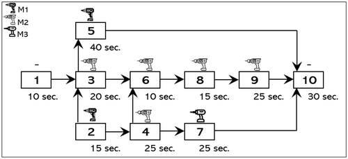
In this section, we describe the ALB problem as the main topic of discussion in the MOLB game before turning to the actual game in Section 4.1. Suppose a manufacturer plans to design an assembly line (i.e., a sequence of working areas known as workstations) that is able to produce 576 units of a single-type product in an eight-hour production shift. Based on the information received from the product design department, for this product, 10 tasks (i.e., elements of work that have to be performed to assemble the product) should be performed according to the precedence diagram presented in Figure 1. The precedence diagram containing nodes and arrows that partially specify the sequence of tasks that has to be considered to be able to perform tasks. For instance, as shown in Figure 1, both tasks 3 and 4 have to be completed before task 6 can be started.
Note. Image icons extracted and modified from Flaticon.com.
Performing each task requires some time, which is called task processing time. Also, each task might need a specific type of cordless power tool that is necessary to perform the corresponding task in the assembly line. The processing time and tool requirement per task are given below and above the corresponding task box, respectively, in Figure 1. There are three different types of cordless power tools labeled M1, M2, and M3. For instance, task 1 does not need a tool; however, tasks 2 and 5 require tool type M1 to be performed by the operator.
Because the production plan is producing 576 units in an eight-hour production shift, then every seconds, one unit of the product should be assembled to meet the production plan. The 50-second time interval is called takt time. To balance the line, we need to assign tasks to workstations such that the precedence restrictions among tasks are not violated and the workload given to each workstation does not surpass the takt time. Figure 2 represents one feasible balance with five workstations/operators and seven cordless power tools that produces exactly 576 units in an eight-hour production shift (i.e., if the interarrival time to the assembly line is set equal to the takt time). See Appendix C to see how the balancing solution presented in Figure 2 is created.

Note. Image icons extracted and modified from Flaticon.com.
As seen in Figure 2, at each workstation, one operator is responsible to perform all the assigned tasks utilizing the required tool at the corresponding workstation. The effectiveness of a balancing solution is evaluated based on the TBL framework by taking the economic, social, and environmental aspects into account. The economic objective can be achieved by minimizing the number of workstations (i.e., a fewer number of workstations is translated into less labor and space costs), the social objective can be achieved by maximizing operator workload smoothness (i.e., a higher operator workload smoothness is translated into more fairness and less ergonomic risks), and the environmental objective can be achieved by minimizing the total number of cordless power tools required for the entire assembly line (i.e., fewer tools are translated into less hazardous materials, such as cadmium and mercury used in the batteries that can contaminate soil and groundwater).
Depending on how each task is assigned to a workstation, the number of workstations as well as the operator workload balance and the number of required tools will be different. For instance, Figures 2 and 3 present two different feasible balancing solutions. By comparing these two balancing solutions, we can observe that Figure 2 presents a more economical balanced line (i.e., it needs five workstations/operators instead of six workstations/operators), whereas Figure 3 presents a more environment-friendly balanced line (i.e., it needs five instead of seven cordless power tools). Moreover, Figure 2 presents a balanced line with a smoother workload division among the workstations/operators.

Note. Image icons extracted and modified from Flaticon.com.
4. An Overview of the MOLB Game
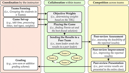
The MOLB game is intended as a team game that can also be played individually. Students are ideally teamed up with three or four students such that there are at least two teams to create a collaborative and competitive atmosphere within and across the teams. Before the instructor shares the game Excel file with the teams, each team should submit its objective weighting parameters based on the team members’ perspective. For example, all team members can assign a weight to each objective, and the average values are taken as the team’s objective weighting parameters. The instructor then initializes the game by sharing the game Excel file with dedicated parameter settings (e.g., takt time, max stdev, tool variety, processing time and tool requirement per task, objective weighing parameters). Notice that, whereas all teams receive the same precedence diagram, all the mentioned parameter values are uniquely generated by the instructor for each team.
Initially, team members play the game individually and try to find as many feasible balances as they can and collect all the feasible balancing solutions. Then, as a team, they bundle all the different feasible solutions found by the team members and form the Pareto solution set and best found solution by eliminating the dominated ones. They should also recheck the feasibility of the solutions in the Pareto solution set and their corresponding objective values to prevent any possible mistakes. By the end of this collaborative session, each team should send a single MOLB file containing the Pareto solution set and the best found solution to a predetermined peer team. We suggest a cycle procedure in which teams are numbered with consecutive numbers, and each team should send its results to the next team with one higher number (e.g., team 2 should send its MOLB file to team 3). The last team should send its file to the first team, and the cycle is complete.
Teams should review the received work in two phases, namely, assessment and improvement. In the assessment phase, they assess if the Pareto solution set contains any non-Pareto solutions, and they check the feasibility of the solutions as well as whether the best found solution is reported correctly. In the improvement phase, the reviewer team can improve the reported results by finding new Pareto solution(s) and a new best found solution. Then, teams should present the results of their review to the entire class by including the received solutions and possible mistakes and improvements found. The instructor can determine the final grade of the teams using at least one of the following two different grading schemes.
Zero-sum scheme: by first awarding 100 points to each team for playing the game and then adding rewards to the peer-review team and subtracting penalties from the reviewed team based on the reward/penalty scheme presented in Appendix A (i.e., for every mistake/improvement found, the peer-review team gains points that are subtracted from the reviewed team).
Additive scheme: by first awarding a base grade (e.g., 60 points or so) to each team for playing the game and then adding peer-review rewards to it based on the reward scheme presented in Appendix A (i.e., for every mistake/improvement found, the peer review team gains points, and they are added to the base grade).
Based on our experience in the classroom, undergraduate students appreciated the zero-sum scheme, whereas the graduate students felt that the zero-sum aspect of the peer reviews was too harsh and preferred the additive scheme. The entire process flow for playing the MOLB game is illustrated and categorized in terms of coordination, collaboration, and competition efforts in Figure 4.
4.1. An Illustration of the MOLB Game
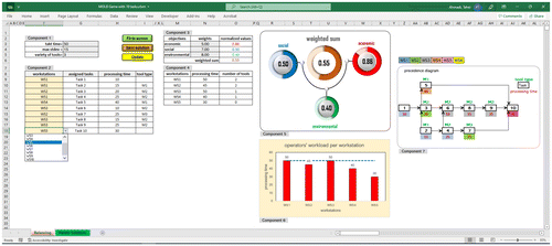
The MOLB game was designed in Microsoft Excel. The game Excel file contains three worksheets, namely, “overview,” “balancing,” and “Pareto solutions” worksheets. After the instructor has set up the game, only the balancing and Pareto solutions worksheets are visible to the students. The former is the main screen of the game, and the latter is used as a placeholder for saving the solutions by the student. For the sake of simplicity, we explain the MOLB game using the 10-task example from Figure 1, whereas the full game includes a 30-task example. Suppose the game is set up with the parameter setting presented in Figure 5 (i.e., entries in cells (G3:G5), cells(N3:N5), and cells(G9:I18)). Students can see three buttons in the balancing worksheet, namely, “fit to screen,” “save solution,” and “update.” The fit to screen button is used when the user wants to fit the working area in the balancing worksheet to its device screen. The save solution is used when the user wants to save a feasible balancing solution in the Pareto solutions worksheet. Finally, the update button is used whenever the user wants to see the most updated entries that are calculated automatically. To explain the functionality of the main components on the main screen of the MOLB game, we label the components as components 1–7 according to Figure 5.
Component 1: This component contains entries for the takt time, max stdev, and variety of tools (i.e., in cells(G3:G5)). This information is randomly generated by the instructor prior to the game and remains static during the student experience.
Component 2: This component contains the list of tasks (i.e., in cells(G9:G18)), their processing time (i.e., in cells(H9:H18)), and tool type requirement (i.e., in cells(I9:I18)). This information is randomly generated by the instructor prior to the game and remains static during the student experience. However, the user should add workstations in cells(F9:F18) manually from a drop-down menu. In this way, the user assigns workstations to the tasks (or, equivalently, tasks are assigned to workstations). This range is shaded with a light yellow color to make it clear to the user that the user needs to do the assignment of tasks to workstations here.
Component 3: This component should not be changed by the user. Entries in cells(N3:N5) are given weights to each objective that are determined by the team members through a class discussion and sent to the instructor prior to the game and remain static during the student experience (i.e., the instructor can randomly generate weights as well). Entries in cells(O3:O6) are the normalized values of the objectives and the weighted-sum value, which are calculated automatically after pressing the update button by the user. Please keep in mind that entries in cells(O3:O6) only show accurate values when the update button is pressed and all the tasks are allocated to workstations in component 2.
Component 4: This component calculates the total processing time and the total number of tools per workstation automatically after pressing the update button by the user. As the user opens more workstations by populating entries in cells(F9:F18) and pressing the update button, component 4 is extended automatically. Please keep in mind that the list of workstations in component 4 always will be in ascending order regardless of the order generated by the user in cells(F9:F18).
Component 5: This component presents the performance of a balancing solution visually to the user in terms of normalized values of economic, social, and environmental objectives as well as the weighted-sum value. All the values are on a scale of zero to one. Zero indicates the worst, and one indicates the best value for each objective. Please keep in mind that the inputs for component 5 come from component 3. The user is not allowed to change or delete component 5.
Component 6: This component provides a visual comparison between the takt time (i.e., a horizontal dashed line in blue) and the workload of the workstations (or operators). The user can judge the feasibility of a balancing solution subject to the takt time constraint. In other words, the user can ensure that the workload of each workstation does not surpass the takt time. The user is not allowed to change or delete component 6. Please keep in mind that the horizontal dashed line for takt time appears when at least two workstations are opened by the user in cells(F9:F18).
Component 7: This component represents the precedence relationship among tasks in a diagram. In addition, the processing time and tool type requirement per task are written below and above each task box, respectively. The structure of this diagram is fixed for all users (i.e., the instructor and students), and its information comes from component 2. However, students can colorize/decolorize the cells within the diagram manually according to a color code to facilitate the recognition of assignable tasks to workstations.
4.1.1. Playing the MOLB Game.
In this section, we explain how a team can play the MOLB game using a 10-task example presented in Figure 5. First, the team members receive the MOLB Excel file with fixed precedence relationships as well as fixed parameters (i.e., the latter are randomly determined by the instructor prior to the game). All the team members can contribute to the team’s achievement by playing the game on their devices independently and creating as many feasible balancing solutions as possible. To create a feasible balance, each team member should follow a step-by-step procedure (Ding et al. 2010). Let us first define available and assignable tasks according to Ding et al. (2010) as follows.
(Available Task). Task 1 is called an available task if and only if task 1 has not already been assigned to a workstation and all of task 1’s predecessors have already been assigned to a workstation (i.e., task 1 doesn’t have any predecessors or all its predecessors are colorized in the precedence diagram).
(Assignable Task). Task 1 is called an assignable task if and only if task 1 is an available task and the idle(remaining) time of the current open workstation is higher than or equal to the processing time of task 1.
Then, the step-by-step procedure for creating a feasible balancing solution can be formulated as follows.
Step 0: Delete all the WSs in component 2 (i.e., entries in cells(F9:F18)), decolorize all the cells within the precedence diagram if they have already been colorized, open WS1 (i.e., ready to assign tasks to WS1), and go to the next step.
Step 1: Determine the available tasks according to the colorized tasks (i.e., assigned tasks) and presented relationships in the precedence diagram and go to the next step.
Step 2: Determine the assignable tasks according to the idle(remaining) time of the current open workstation and processing time of the available tasks and go to the next step.
Step 3: If there is at least one assignable task, go to the next step; otherwise, go to step 5.
Step 4: Select a task from the assignable tasks (i.e., if there is more than one assignable task, prioritize them based on your preferred heuristic rule) and assign it to the current open workstation (i.e., colorize the task in the precedence diagram and add the open WS from the drop-down menu to the selected assignable task in component 2), press the update button and go back to step 1.
Step 5: If there is at least one available task, go to the next step; otherwise, go to step 7.
Step 6: Close the current open workstation (i.e., do not assign tasks to it anymore), press the update button, and open the next workstation and go back to step 1.
Step 7: Stop the procedure, press the update button first and then the save solution button.
By following the step-by-step procedure and reaching step 7, the student has created a feasible balancing solution. By executing step 7, the feasible balancing solution and its corresponding normalized objective values are saved in the Pareto solutions worksheet. To create a new feasible balancing solution, the student needs to restart the procedure and try to allocate tasks to workstations differently than what the student did in the previous feasible balancing solution (i.e., use different heuristic rules for prioritizing assignable tasks in step 4). In Appendix C, we provide a walkthrough for the population of WS1 in the game Excel file with the 10-task example presented in Figure 5 using the aforementioned step-by-step procedure.
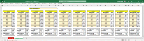
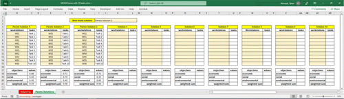
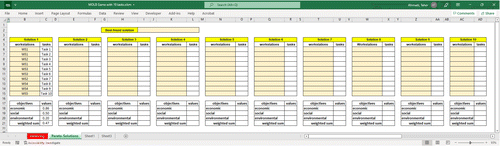
Each team member should play the game independently and try to find as many feasible balancing solutions as possible and save them in their Pareto solutions worksheet. When the team members feel that they have generated enough feasible balancing solutions (i.e., for some this might mean five, for others as many as twenty), they can stop the search and turn their focus to forming their Pareto solution set. They first need to bundle all different feasible solutions as shown in Figure 6. Please keep in mind that feasible solutions 1 and 5 are not the same balancing solution even though they have the same normalized objective values and weighted-sum value (e.g., task 3 has been assigned to different workstations in solutions 1 and 5). Next, the team needs to review their final feasible solution set to reach a Pareto solution set by comparing all the feasible solutions two by two in terms of their economic, social, and environmental objective values and eliminating dominated solutions. First, let us define the dominance and Pareto solution set concepts according to Figueira et al. (2010).
(Dominance). Solution II dominates solution I if and only if solution II is no worse than solution I in all objectives and solution II is strictly better than solution I in at least one objective.
(Pareto Solution Set). A set of feasible solutions in which none of them are dominated by the others.
Based on Definition 3, the feasible solution set presented in Figure 6 can be edited and changed to a Pareto solution set. To do so, we need to compare all the feasible solutions two by two. For instance, feasible solution 1 is dominated by feasible solution 2 (i.e., equivalently, solution 2 dominates solution 1). Then, solution 1 should be removed from the Pareto solutions worksheet. Solution 2 does not dominate solutions 3 and 4. However, it dominates solution 5. Thus, solution 5 should be removed from the Pareto solutions worksheet as well. By comparing all the feasible solutions two by two and removing all the dominated ones, feasible solutions 2, 3, and 4 remain. These solutions can be labeled as Pareto solutions 1, 2, and 3, respectively, as presented in Figure 7. In addition, by comparing the weighted-sum value of the Pareto solutions, Pareto solution 2 with the highest weighted-sum value is reported in cell(I2) as the best found solution of the team. Then, the file is saved and sent to the reviewer team as the final result of the team.
4.1.2. Incorporating Three Objectives into a Decision.
Let’s now consider more closely how the three objectives are weighted in the decision-making process. Obviously, the economic, social, and environmental objective values have different scales. Therefore, we first need to normalize them. Let Ni indicate the value of objective i, , on a scale of , where Ni = 0 shows no achievement and Ni = 1 shows a full achievement of objective i.
The economic objective measures the effective usage of resources (e.g., labor and space) in the balanced line. Then, its minimum value occurs when every single task is assigned to a dedicated workstation, and its maximum occurs when the same workload as the takt time is assigned to all the workstations (i.e., ). The economic objective is measured in terms of line efficiency. Let be the line efficiency. Then,
The social objective measures the fairness of the workload distribution among the workers in the balanced line. Its maximum occurs when all the workstations have the same workload (i.e., ). For the minimum of the social objective, we define a threshold that appears in the game Excel file as the “max stdev” parameter. Hence, the standard deviation of the workloads across workstations at max stdev and beyond, makes fairness meaningless (i.e., ). The social objective is determined in terms of the standard deviation of the workloads across the workstations. Let be the standard deviation of the workloads across the workstations, and then,
The environmental objective measures the effective usage of cordless power tools that can harm the environment with hazardous materials, such as cadmium and mercury used in the batteries. Its maximum occurs when all the tasks are assigned to one workstation (i.e., ), and its minimum occurs when all the tasks with a tool requirement are assigned to different workstations (i.e., ). The environmental objective is measured in terms of the total number of tools needed for the balanced line. Let be the total number of tools needed for the entire balanced line. Then,
Finally, the weighted-sum value corresponding to a balance decision can be calculated by incorporating the decision maker’s preferences. Let be the given weight to objective i, and then,
In the game Excel file, components 4 and 5 in the balancing worksheet are dedicated to calculating and presenting the normalized objective values.
4.1.3. Strategies for Improving Objective Functions.
In this section, we provide some heuristic-based rules that students can use to prioritize assignable tasks (i.e., in step 4 of the step-by-step procedure) to improve each of the three objective functions. This information can be shared by the instructor either before the students attempt to find feasible ALB solutions, when they are working on it, or only in the peer-review stage when students are trying to improve on their peers’ solutions.
4.1.3.1. Economic Objective.
Achievement of the economic objective may be measured in terms of line efficiency. Hence, a lower number of workstations leads to the higher achievement of the economic objective. It is noteworthy that the theoretical minimum number of workstations is a lower bound for the optimal number of workstations, and the theoretical minimum number of workstations is calculated as
4.1.3.2. Social Objective.
Achievement of the social objective may be measured by the variation (standard deviation) in workload distributions among the workstations. Less variation among the workloads relates to the higher achievement of the social objective. Notably, all the ALB heuristic procedures are greedy in assigning as much work as possible to the early workstations to reduce the number of workstations and maximize the economic objective. This leads to more idle time for later workstations and, in turn, a more imbalanced workload across workstations and lower social objectives. To overcome this issue, the student might need to overrule the heuristic rules for improving the economic objective to give an even workload to all workstations and maximize the social objective as well.
4.1.3.3. Environmental Objective.
Achievement of the environmental objective may be measured in terms of the total number of tools required for the entire line. Grouping tasks with common tool requirements may decrease and lead to the higher achievement of the environmental objective. A heuristic rule for improving the environmental objective can be prioritizing assignable tasks based on their tool-type similarity with the assigned tasks to the current open workstation (i.e., tool variety reduction within each workstation). For instance, suppose a task with a tool requirement of type M1 was already assigned to the current open workstation and two assignable tasks exist with tool requirements of type M1 and M2. Then, the assignable task with tool type M1 gets a higher priority compared with the other assignable task for the assignment to the open workstation because it results in less tool variety in the open workstation and, in turn, fewer total tools for the entire production line.
Remember that the aforementioned heuristic rules are for improving just one objective. During the game, students need to integrate the heuristic rules to be able to improve two or all three objectives simultaneously. As far as the authors are aware, such combined heuristics that improve two or even three objectives simultaneously do not exist in the literature, which makes this game a unique challenge to the students that closely mimics real-life decision making.
5. Learning Outcomes of the Game
By playing the MOLB game, students actively learn about ALB, the TBL framework, ST, and the MCDM concepts. We explain each of these three learning outcomes briefly.
By playing the game, students are practicing ALB by finding feasible balance decisions, repetitively. This means that students are practicing making a tactical decision on matching supply with the market demand. In essence, students are learning how to design an assembly line based on a product layout process configuration (i.e., flow shop). Students learn how to assign tasks to a set of sequential workstations such that the workstations’ workloads don’t surpass predetermined takt time on the one hand and the precedence relationships among tasks are not violated on the other. In other words, team members are trying to find as many feasible balances as possible and give prompt feedback to each other in case finding a feasible balance has not been understood by all the team members properly.
In the MOLB game, the economic objective measures the effective usage of resources (e.g., labor and space), the social objective measures the fairness of the workload distribution among the operators, and the environmental objective measures the effective usage of tools (i.e., assuming that batteries in cordless power tools contain destructive materials to the environment) in the production line. As such, students get familiar with the economic, social, and environmental aspects of ALB known as the TBL framework. Given that they have to balance these three objectives simultaneously, students also get introduced to the MCDM concept.
Team members discuss all the found feasible balancing solutions to form the Pareto solution set. To do so, they need to compare the feasible solutions with each other and eliminate all the dominated ones to form the Pareto solution set. Then, they need to look at the weighted sum of the Pareto solutions to determine the best found solution with regard to the given weights to the objectives. By going through this process, team members are sharing their understanding of these concepts and providing prompt feedback to each other. This also means that students are introduced to an ST approach that looks beyond a simple solution to a straightforward problem.
6. Evidence of the MOLB Game Effectiveness
In this section, we test the effectiveness of the MOLB game by surveying the graduate and undergraduate students who played the game. Next, we benchmark the MOLB game against other well-known games that are played by business schools around the globe.
6.1. Surveying the Students
We have used the MOLB game in the operations management course at the undergraduate level as well as in the operations and supply chain management course at the graduate level. We have played the MOLB game with teams of four students. Each team received an MOLB game Excel file containing the same precedence diagram with 30 tasks and three different types of tools. The precedence relationships were fixed, but everything else was randomly generated by the instructor per team.
We started the first session with a 15-minute introduction to the game using the 10-task example presented in this paper. Then, teams started working on their unique problem in the same way as discussed in Section 4.1.1. In a second session, each team conducted the peer reviews. Then, each team made a 10-minute presentation to present their review effort to the entire class in the third session. Please note that we always awarded grades based on the zero-sum structure in Appendix A. As previously discussed, the graduate students particularly objected to this, so the additive scheme might be more useful.
We observed that students were actively engaged and provided feedback to each other in the team. Interestingly, we noticed that a substantial number of teams made a mistake when they generated their Pareto solutions themselves, whereas they noticed similar types of mistakes in the work of their peers. This means that the learning process was also happening during the peer review. After playing the game, we surveyed the students anonymously and ask students’ opinions on the effectiveness of the MOLB game by asking the following questions similar to Snider et al. (2017).
Learning about ALB: After playing this game, I am confident that I can determine a feasible solution for an ALB problem.
Learning about the TBL framework: By playing the game, I learned how the TBL framework can be incorporated into business decisions.
Learning about MCDM concept: By playing the game, I learned how a final decision can be made by incorporating different objectives.
Learning through collaboration: Playing in a team helped me to learn even more by having discussions with teammates.
Learning through competition: The zero-sum grading policy (i.e., gaining the same points that another team loses) encouraged me to put more effort and learn more.
Effectiveness of peer review: Evaluating what the other teams proposed helped me to learn even more about the ALB concept.
Superiority of the MOLB game over lecturing: I enjoyed learning about ALB through this game more than I would have through a traditional lecture.
The MOLB game satisfaction: What is your overall satisfaction rating for the game (out of 10)?
Questions 1–7 were developed based on a five-point Likert scale from strongly disagree to strongly agree. Question 8 captured students’ overall satisfaction on a scale of 0 to 10. We also asked, “Do you have any suggestions for improving the game?” as an open question to collect students’ views and suggestions regarding the improvement of the MOLB game. A sample of students’ suggestions can be found in Appendix B. Tables 1 and 2 represent the results of questions 1–7 for undergraduate and graduate students who played the game.
|

Table 1. Undergraduate Students Survey Results
| Questions | −2 | −1 | 0 | 1 | 2 | Total | Mean | % − (%) | % 0(%) | % + (%) |
|---|---|---|---|---|---|---|---|---|---|---|
| Learning about ALB | 0 | 0 | 1 | 9 | 27 | 37 | 1.70 | 0.0 | 2.7 | 97.3 |
| Learning about the TBL framework | 0 | 0 | 1 | 13 | 23 | 37 | 1.59 | 0.0 | 2.7 | 97.3 |
| Learning about MCDM concept | 0 | 0 | 1 | 16 | 21 | 38 | 1.53 | 0.0 | 2.6 | 97.4 |
| Learning through collaboration | 0 | 2 | 2 | 10 | 22 | 36 | 1.44 | 5.6 | 5.6 | 88.9 |
| Learning through competition | 1 | 3 | 4 | 10 | 18 | 36 | 1.14 | 11.1 | 11.1 | 77.8 |
| Learning through peer review | 0 | 0 | 3 | 9 | 24 | 36 | 1.58 | 0.0 | 8.3 | 91.7 |
| Superiority of the MOLB over lecturing | 0 | 0 | 0 | 5 | 31 | 36 | 1.86 | 0.0 | 0.0 | 100.0 |
Note. Average overall MOLB game satisfaction: 8.6 out of 10.
|
Table 2. Graduate Students Survey Results
| Questions | −2 | −1 | 0 | 1 | 2 | Total | Mean | % − (%) | % 0(%) | % + (%) |
|---|---|---|---|---|---|---|---|---|---|---|
| Learning about ALB | 1 | 5 | 4 | 30 | 42 | 82 | 1.30 | 7.3 | 4.9 | 87.8 |
| Learning about the TBL framework | 1 | 7 | 10 | 33 | 32 | 83 | 1.06 | 9.6 | 12.0 | 78.3 |
| Learning about MCDM concept | 2 | 3 | 4 | 32 | 43 | 84 | 1.32 | 6.0 | 4.8 | 89.3 |
| Learning through collaboration | 3 | 3 | 8 | 24 | 44 | 82 | 1.26 | 7.3 | 9.8 | 82.9 |
| Learning through competition | 10 | 11 | 12 | 21 | 27 | 81 | 0.54 | 25.9 | 14.8 | 59.3 |
| Learning through peer review | 9 | 8 | 12 | 22 | 31 | 82 | 0.71 | 20.7 | 14.6 | 64.6 |
| Superiority of the MOLB over lecturing | 4 | 7 | 3 | 20 | 47 | 81 | 1.22 | 13.6 | 3.7 | 82.7 |
Note. Average overall MOLB game satisfaction: 7.4 out of 10.
The results clearly show the students’ appreciation for our MOLB game in all its aspects, perhaps most notably in its superiority over normal lectures. We can also observe that the undergraduate students were more positive about the game than the graduate students, particularly regarding learning through competition. Based on our experience in the classroom, undergraduate students appreciated the zero-sum scheme, whereas the graduate students felt that the zero-sum aspect of the peer reviews was too harsh and preferred the additive scheme
6.2. Benchmarking
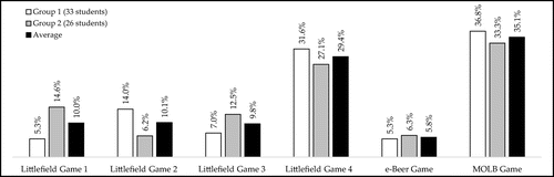
In addition to our MOLB game, we also played other web-based simulation games in our courses. These web-based simulation games are known as Littlefield and the eBeer game. We played four rounds of the Littlefield game (Snider and Balakrishnan 2013, Lojo 2016). In the academic year 2020–2021, two groups of 40 undergraduate students played four rounds of the Littlefield game individually and the e-Beer and MOLB game in teams of four students. We surveyed all students anonymously to determine their favorite game among these six games. As can be observed from Figure 8, our students were more satisfied with playing the Excel-based MOLB game compared with the other web-based simulation games that are well-known games and played by various business schools around the globe.
7. Teaching Experience
We have played our MOLB game at the undergraduate and graduate levels six times (i.e., in total >70 teams) so far. No technical or other issues were reported by the students. Because we used the precedence diagram with 30 tasks, there is an almost infinite set of feasible balances, and therefore, students always found room for improvement in the peer-review round. We experienced that the parameter setting of the MOLB game can be customized per team by the instructor with very little effort and time by pressing the “set the parameters” button in the master file of the game. The MOLB game Excel file can be shared with the teams via available information-sharing platforms or directly via email. We observed that providing a 15-minute overview of the game helps students reduce their fears and get started in the right direction. This fact has also been echoed by Snider and Balakrishnan (2013).
Because we played the game in teams of four students, it was interesting that we did not receive any complaints regarding free-riders within the teams because everyone could contribute to the achievement of the team by playing the game individually. Based on students’ feedback and comments received from the anonymous survey, the MOLB game was recognized as a user-friendly and easy game to play. The peer-review evaluations were constructive as we frequently observed that a team had poor performance (e.g., reported infeasible solutions and not a reliable Pareto solution set) when they played the game, whereas they did a wonderful job when they reviewed a peer’s work and providing feedback on very similar mistakes that they made themselves in the first round of playing the game. Even though some students criticized the zero-sum scheme for grading the game, we noticed that students were engaged and were able to reflect on their work when the peer team presented their findings and improvements with them.
We thank the editor, associate editor, and the anonymous referees for their constructive suggestions that substantially improved the quality of the paper and the game Excel worksheets. Furthermore, we thank all the students who played the game and provided feedback and comments either in class or through anonymous surveys.
Appendix A. Grading Scheme
The reviewer team is rewarded for finding any mistakes or possible improvements according to the following scheme, and the team that owns the work is penalized with similar points. The review process for the MOLB game should be done in two phases:
Assessment phase: The reviewer team needs to check the feasibility of all the reported results. This means checking if
• The Pareto solution set contains non-Pareto solutions (±5 points for each case).
• The best found solution is determined incorrectly (±5 points).
• The workload of the workstations surpasses the takt time (±5 points for each case).
• The objective values and total are reported incorrectly (±2 points).
• The precedence relationship among tasks is violated (±5 points for each case).
Improvement Phase: The reviewer team can improve the reported results by finding
• New Pareto solutions (±10 points for each).
• New best found solution (±5 points).
In case the reviewer team is not eligible for a reward, the results can be reviewed by the instructor. In this case, any findings by the instructor result in double penalties for the reviewer team and the same penalties mentioned in the grading schemes.
Appendix B. Feedback on the Game by the Students
Here, we share some appreciation and constructive feedback by students (i.e., both undergraduate and graduate students who played the game) on the MOLB game collected through anonymous surveys.
Appreciation feedback:
I don’t have any suggestions, it was pretty entertaining!
I don’t have any suggestions. I think it works really well, and the way it works is really nice! The game was very nicely designed, I had a lot of fun playing!
No suggestions. I really enjoyed playing this game as a team. We spent so much time on this game because we really liked it, thank you for the class!!
No suggestions at the moment, thank you so much!
I have no suggestion to improve the game, it was the first time I played this kind of game and I really learned a lot from it. Thank you very much for this class.
No further suggestions. I really enjoyed learning more about ALB interactively. I think it was an awesome game, and if you had put time and effort into it, it is doable and understandable.
It was a well-thought-out game! It might be a better idea to create a different grading system than a zero-sum scheme.
No suggestions. I think the game was good and fun, maybe some extra explanation about some terminologies, such as Pareto and best-found decisions.
No suggestions. It was a great game, and I enjoyed it as well as the grading part.
No specific suggestions. I thought that everything was really clear and easy to work with. I had a lot of fun, and the different concepts and definitions became really clear because of playing the game.
We really enjoyed the game, and it was really educational!
No suggestions. I did learn more knowledge of ALB when playing this game. Thank you for designing this game.
Personally, I feel that the MLOB game is a great addition to the OSCM course.
No suggestions. Please keep it in the course.
Very fun to play it!
Constructive feedback:
Find a way to notify automatically if a solution is not feasible because of violating the precedence relationship among tasks!
Automatic colorizing of the tasks in the precedence diagram when they are allocated into workstations.
Play the game in the middle of the term and not the last days before the exams!
I do not like that one team (the owner of the work) loses points while the reviewer team gets them. Maybe only give the reviewer team points for their review and don’t subtract them from the owner of the work.
I would suggest sharing the peer-review results by the reviewer team with the owner of the work one day before the presentation session. So the owner of the work has enough time to evaluate the accuracy of the peer-review results.
First of all, I want to say that I’m very impressed by the way that you invented the game. However, I did not like very much the zero-sum grading scheme in which one team gets points from the other team!
I think it was a great way to understand this topic. It could be helpful to understand how we could make such an Excel file.
Make it less abstract, not only numbers in Excel but a real story behind the game.
Appendix C. Creating a Feasible Balancing Solution Using the MOLB Game
Here, we illustrate how the step-by-step procedure for creating a feasible balancing solution is applied by providing a walkthrough for the population of the first workstation in the game Excel file for the 10-task example.
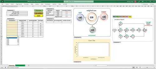
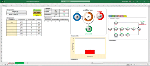
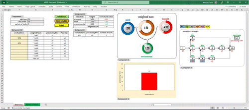
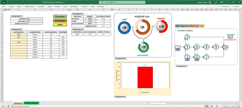
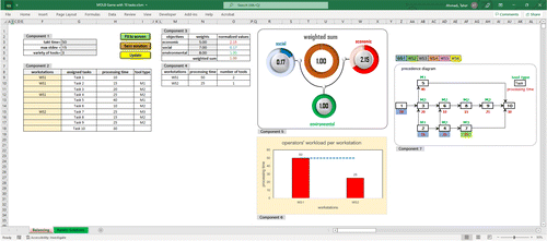
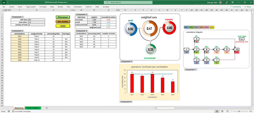
For step 0 as seen in Figure C.1, there are no entries in cells(F9:F18), and the cells within the precedence diagram are not colorized. Then, we open WS1 (i.e., ready to assign tasks to it) and go to step 1. In step 1, we need to look at the precedence diagram and try to find the available tasks. As is seen from the precedence diagram, tasks 1 and 2 are the only available tasks for now because they have no precedence tasks and they have not been assigned to a workstation yet. Then, we need to go to step 2. For step 2, because the processing time of both available tasks are less than or equal to the idle time of WS1 (i.e., because no tasks have been assigned to WS1 yet, it has an idle time equal to the takt time), both tasks 1 and 2 are assignable. Then, we need to go to step 3. In step 3, because there are two assignable tasks, we need to go to step 4. In step 4, we can choose either task 1 or 2. Let’s choose task 2 according to the LCR heuristic rule (i.e., it has a bigger processing time) and assign it to WS1. To do so, as is presented in Figure C.2, we need to first colorize cell(AB19) in blue manually (i.e., according to the predefined color code above the precedence diagram) and then populate an entry in cell(F9) by clicking on the cell and choosing WS1 from the drop-down menu and pressing the update button. By doing so, task 2 is allocated to WS1, and a summary of WS1 is given in component 4. Then, we need to go back to step 1. Please keep in mind that, because we have not assigned all the tasks to workstations, the normalized objective values in components 3 and 5 are not accurate. In step 1, from the precedence diagram presented in Figure C.2, we see that tasks 1 and 4 are the available tasks. Then, we need to go to step 2. In step 2, based on the idle time of WS1 (i.e., 50 − 15 = 35) and the processing time of available tasks, we see that both tasks 1 and 4 are assignable. Then, we need to go to step 3. In step 3, because there are two assignable tasks, we need to go to step 4. In step 4, we can choose either task 1 or 4. Let us choose task 4 according to the LCR heuristic rule (i.e., it has a bigger processing time) and assign it to WS1. To do so, as is presented in Figure C.3, we need to first colorize cell(AD19) in blue (i.e., according to the predefined color code above the precedence diagram) and then populate an entry in cell(F12) by clicking on the cell and choosing WS1 from the drop-down menu, and press the update button. By doing so, task 4 is also allocated to WS1 and a summary of WS1 is given in component 4. Then, we need to go back to step 1. In step 1, from the precedence diagram presented in Figure C.3, we see that by assigning tasks 2 and 4 to WS1, tasks 1 and 7 become available tasks. Then, we need to go to step 2. In step 2, based on the idle time of WS1 (i.e., 50 − 40 = 10) and the processing time of available tasks, we see that just task 1 is assignable. Then, we need to go to step 3. In doing step 3, because there is one assignable task, we need to go to step 4. In step 4, because there is just one assignable task, we assign task 1 to WS1. To do so, as is presented in Figure C.4, we colorize cell(Z15) in blue, populate an entry in cell(F9) by clicking on the cell and choosing WS1 from the drop-down menu and pressing the update button. By doing so, task 1 is also allocated to WS1. Then, we need to go back to step 1. In doing step 1, from the precedence diagram presented in Figure C.4, we see that by assigning tasks 1, 2, and 4 to WS1, tasks 3 and 7 are the available tasks. Then, we go to step 2. In step 2, because the idle time of WS1 is zero and zero is less than the processing time of available tasks 3 and 7, there is no assignable task. Then, the following occurs. In step 3, because there is no assignable task, we need to go to step 5. In step 5, because tasks 3 and 7 are available, we need to go to step 6. In step 6, we need to open WS2 (i.e., ready to assign tasks to it) and go back to step 1. For step 1 from the precedence diagram presented in Figure C.4, we see that tasks 3 and 7 are the available tasks. Then, we need to go to step 2 in which the idle time of WS2 is 50, and 50 is more than the processing time of available tasks, both tasks 3 and 7 are assignable tasks. Then, we need to go to step 3. In step 3, because there are two assignable tasks, we need to go to step 4. In step 4, we can choose either task 3 or 7. Let’s choose task 7 according to the LCR heuristic rule (i.e., it has a bigger processing time) and assign it to WS2. To do so, as is presented in Figure C.5, we need to first colorize cell(AF19) in green (i.e., according to the predefined color code above the precedence diagram) and then populate an entry in cell(F15) by clicking on the cell and choosing WS2 from the drop-down menu and pressing the update button. By doing so, task 7 is also allocated to WS2, and a summary of WS1 and WS2 is given in component 4. Then, we need to go back to step 1. By continuing the procedure, all the nonassigned tasks can be assigned to WS2, WS3, WS4, and WS5 in the same way that tasks were assigned to WS1. When we reach step 7, we have created a feasible balancing solution (see Figure C.6). By executing step 7 and pressing the save solution button, the feasible balancing solution is saved in the Pareto solutions worksheet as presented in Figure C.7, and a confirmation message box appears on the screen. The user needs to press “OK” to close the message box.
References
- (2018) Workload smoothing in simple assembly line balancing. Comput. Oper. Res. 89:51–57.Crossref, Google Scholar
- (2010) Kolb’s experiential learning model: Critique from a modelling perspective. Stud. Continuing Ed. 32(1):29–46.Crossref, Google Scholar
- Ding LP, Feng YX, Tan JR, Gao YC (2010) A new multi-objective ant colony algorithm for solving the disassembly line balancing problem. Internat. J. Advanced Manufacturing Tech. 48(5):761–771.Google Scholar
- (2021) Design and management of assembly systems 4.0: Systematic literature review and research agenda. Internat. J. Production Res. 60(1):184–210.Crossref, Google Scholar
- (1994) Toward the sustainable corporation: Win-win-win business strategies for sustainable development. California Management Rev. 36(2):90–100.Crossref, Google Scholar
- (2022) Teaching systems thinking in higher education. INFORMS Trans. Ed. 22(2):66–102.Link, Google Scholar
- (2012) Flow index based line balancing: A tool to improve the leanness of assembly line design. Internat. J. Production Res. 50(12):3345–3358.Crossref, Google Scholar
- (2008) Modeling multi-objective multi-stakeholder decisions: A case-exercise approach. INFORMS Trans. Ed. 8(3):103–114.Link, Google Scholar
- Figueira JR, Liefooghe A, Talbi EG, Wierzbicki AP (2010) A parallel multiple reference point approach for multi-objective optimization. Eur. J. Oper. Res. 205(2):390–400.Google Scholar
- (2020) Workers’ rest allowance and smoothing of the workload in assembly lines. Internat. J. Production Res. 58(4):1255–1270.Crossref, Google Scholar
- Groover MP (2016) Automation, Production Systems, and Computer-Integrated Manufacturing (Pearson Education India).Google Scholar
- Helgeson W, Birnie DP (1961) Assembly line balancing using the ranked positional weight technique. J. Indust. Engrg. 12(6):394–398.Google Scholar
- (2020) Case—The fendt variotakt: Revolutionizing mixed-model assembly line production. INFORMS Trans. Ed. 20(3):141–153.Link, Google Scholar
- (2007) Charging up the batteries: Squeezing more capacity and power into the new EU battery directive. Comput. Law Security Rev. 23(4):357–364.Crossref, Google Scholar
- Kilbridge M, Wester L (1961) A heuristic method of assembly line balancing. J. Indust. Engrg. 12(4):292–298.Google Scholar
- (2019) Active game-based learning of dynamics modeling and simulation in biomedical systems engineering. INFORMS Trans. Ed. 20(1):16–25.Link, Google Scholar
- Lojo MP (2016) Improving undergraduate student performance on the littlefield simulation. INFORMS Trans. Ed. 16(2):54–59.Google Scholar
- (2015) Heuristics and lower bounds for the simple assembly line balancing problem type 1: Overview, computational tests and improvements. Eur. J. Oper. Res. 240(1):32–42.Crossref, Google Scholar
- (2012) Examining the effectiveness of experiential teaching methods in small and large OM modules. Internat. J. Oper. Production Management 32(12):1473–1492.Crossref, Google Scholar
- (1991) Improving the equality of workload assignments in assembly lines. Internat. J. Production Res. 29(3):619–633.Crossref, Google Scholar
- (2004) On modeling line balancing problems in spreadsheets. INFORMS Trans. Ed. 4(2):45–48.Link, Google Scholar
- (1997) Simple assembly line balancing-heuristic approaches. J. Heuristics 2(3):217–244.Crossref, Google Scholar
- Snider B, Balakrishnan J (2013) Lessons learned from implementing web-based simulations to teach operations management concepts. INFORMS Trans. Ed. 13(3):152–161.Google Scholar
- (2017) Student peer evaluated line balancing competition. INFORMS Trans. Ed. 17(2):43–48.Link, Google Scholar
- (1986) A comparative evaluation of heuristic line balancing techniques. Management Sci. 32(4):430–454.Link, Google Scholar
- (2013) Teaching note-implementing line balancing heuristics in spreadsheets. INFORMS Trans. Ed. 13(2):114–125.Link, Google Scholar
- (2018) Interactive Excel-based procedure for line balancing. INFORMS Trans. Ed. 19(1):23–35.Google Scholar
- (1986) Optimal system design with multiple criteria: De novo programming approach. Engrg. Costs Production Econom. 10(1):89–94.Crossref, Google Scholar

