Case—Racial Bias in Automated Traffic Law Enforcement and the Price of Unjustness
Abstract
This case study has been developed for students to practice their data analysis and optimization skills in a contemporary societal issue: that of injustice in automated traffic law enforcement. Specifically, this case study is for students of modern data analysis and statistical modeling courses that focus on hypothesis testing; it also has a component for students in optimization and mathematical modeling courses that focus on linear and network optimization. The case study has been used since Spring 2023 in a combination of two courses from the Industrial Engineering (Analysis of Data, an introduction to probability and statistics) and Civil Engineering (Transportation Systems, an introduction to mathematical modeling and optimization for civil engineers with a focus on transportation) curricula.
History: This paper has been accepted for the INFORMS Transactions on Education Special Issue on DEI in ORMS Classrooms.
1. Introduction
The purpose of this case study is to use real-life data to perform a full hypothesis testing and solve an optimization problem with societal and justice implication. First, we introduce a timely societal issue that combines notions from transportation engineering, law enforcement, and racial injustice. Then, students are asked to formulate a suitable statistical hypothesis to see whether a specific automated law enforcement tool can, in fact, be unjust for part of the population. At this step, students use real-world data and the Python pandas package to collect the necessary information and use them in the context of hypothesis testing. Students are also asked to rethink how shortest path problems need to be formulated to capture side-constraints emerging from automated traffic law enforcement system biases. Finally, after this case study, students have a better understanding how numerous policies have unintended consequences and discuss as a group ways to use data analysis and network optimization to improve policy outcomes. Specifically, the objectives of this case study are as follows:
O1. Read data using the pandas package and visualize summary statistics using matplotlib.
O2. Estimate probabilities and conditional probabilities using real-world data.
O3. Formulate relevant statistical hypotheses and devise a plan to collect and use data to reject or fail to reject them.
O4. Derive meaningful analyses from our statistical hypotheses and report useful information such as P-values and errors.
O5. Mathematically model problems on networks, such as the shortest path problem and the constrained shortest path problem, inspired by contemporary issues in urban traffic law enforcement.
O6. Use linear optimization and open-source optimization solvers (such as PuLP) to solve unconstrained and constrained shortest path problems on networks.
O7. Critically analyze the results from linear optimization as a tool to evaluate and critique disparities and injustice.
Additionally, the case study is at the intersection of various areas of study, including the following:
A1. Statistics and data analytics.
A2. Operations research.
A3. Transportation engineering and systems.
A4. Justice and law enforcement.
Although the case study is meant to be taught so that engineering students are primarily exposed to these areas, some areas may be more or less pronounced in each of the questions. We mark each question with the appropriate areas to make this conversation easier.
2. Are Red Light Cameras Racist?
If you have ever driven a vehicle in the state of Illinois, then chances are you have observed cameras in certain intersections. These serve to automatically monitor certain traffic safety laws, such as failing to stop at a red light and/or speeding, especially in locations where traffic stops are difficult to perform (Goodwin et al. 2015, Centers for Disease Control and Prevention 2022). As of October 2023, there are 336 communities across 23 states and the District of Columbia that employ cameras as a law enforcement tool (Insurance Institute for Highway Safety (IIHS) 2023). Chicago, Illinois, and its surrounding areas are among these communities and we will be using data from the city of Chicago in our analysis. Figure 1 shows a map of the United States with all states that are using traffic cameras for traffic law enforcement.
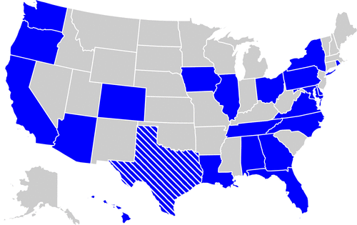
Note. Texas (shown in striped blue) has a state law disallowing the use of red light cameras since June 2019; however, it also has communities that are permitted the use due to preexisting contracts in place.
What is our motivation? ProPublica made a pretty daring claim that Chicago’s supposedly “race-neutral” traffic cameras “disproportionately ticket Black and Latino motorists” (Hopkins and Sanchez 2022). If this is true, it affects how people transport themselves in the community as Black and Latino drivers would be more prone to avoiding certain areas; it would affect access to opportunities in Chicago and its surrounding areas; and it would also lead to economically ruining citizens and residents (Sanchez and Kambhampati 2018). Seeing as more cities and states are advocating using traffic cameras, we can see how a sound scientific statistical analysis is necessary and timely and how you are the best-equipped to do it.
2.1. The Story of Ameenah1
As an extra motivation for studying this problem, we present a story that is not that uncommon for many drivers in Chicago. Ameenah is a lifelong Chicago resident who left for college before returning to Chicago for work. Her position requires her to drive in and around the city, as well as make multiple stops in a day. Although she is driving the same way as when she used to commute to school, she is now amassing more tickets: All of them come through the mail, and all of them are from a camera in one of the intersections she has crossed. Specifically, Ameenah has on “red light” camera violation and five “high speed” violations from a radar, for a total cost of $600. Although she counts herself lucky to be able to afford that, she cannot stop thinking that something is amiss.
2.2. Data
In the remainder of this case study (and to help Ameenah figure out whether something is truly amiss with the automated traffic law enforcement systems in Chicago), you will need a series of data. First, we need access to the data files from the ProPublica investigation that includes information about every ticket issued automatically by a traffic camera in Chicago, Illinois, since 2010. These files can be accessed through here: https://www.propublica.org/datastore/dataset/city-of-chicago-camera-tickets-and-warnings-data; we are also providing you with the necessary information in a series of text files called “year.txt” where year. As an example, file “2019.txt” would include all necessary data for tickets issued in 2019. The data set includes multiple interesting information, as shown in Table 1. In this case study, we will specifically focus on only a few of the fields.
|

Table 1. Data Set Fields and Their Format
| Field | Description |
|---|---|
| ticket_number | Citation ID |
| issue_date | Date (DD/MM/YY) and time of ticket |
| violation_location | Location (street address) of ticket |
| violation_code | Code associated with violation |
| violation_description | Description of violation |
| zipcode | ZIP code (in xxxxxyyyy, where xxxxx is the five digit zip code) associated with the vehicle registration |
| unit | Abbreviated camera unit type. Marked as “SPD” for speed camera violations, “RDFX”, “CDNT”, or “XERX” for red-light camera violations. |
| unit_description | Unabbreviated camera unit type. |
| officer | Similar to unit. Marked as “SPEED” for speed camera violations, and “RDFX” or “XERX” for red-light camera violations. |
| vehicle_make | The make of the vehicle ticketed. |
| license_plate_type | Type of vehicle ticketed. The vast majority will be “PAS” (passenger), however also included are commercial vehicles like trucks or taxis (e.g., “TRT”, or “TXI”), temporary plates (“TMP”), and others. |
| fine_level1_amount | Original citation cost. |
| fine_level2_amount | Citation cost after including late penalty fees. |
| current_amount_due | Total amount due after including late penalty fees and after accruing a 22% collection charge. |
| total_payments | Total amount paid. |
| ticket_queue | Most recent status of the ticket (e.g., paid, dismissed, hearing, etc.). |
| ticket_queue_date | Date of latest status update. |
| notice_number | Unique notice ID. |
| notice_level | The notice that was sent to the driver, including “VIOL” (for violation), “SEIZ” (when the vehicle is to be booted), “FINL” (final disposition and ticket is sent to collections). The field could be blank (i.e., no notice). |
| hearing_dispo | Hearing outcome/disposition, finding a driver “liable” or “not liable”. The field could be blank if the driver never contested the ticket. |
| hearing_reason | Reason of ticket dismissal, if the ticket was dismissed. If the ticket was either not contested (i.e., no hearing) or if the driver was found liable, this field is blank. |
Note. All fields are separated through the use of a “$” as a separator character.
[
Using pandas, read the data set, ignoring any observations without a zip code. Recall that the data are separated using a “$”, so use the separator argument in the pandas read_csv functionality [O1].
Report the number of notices in your data set [O1].
Time for a conditional probability calculation: what is the probability that a hearing finds the driver not liable? That is, among the drivers that contested the ticket, what fraction found them not liable [O2]?
Use your earlier calculation to answer the following question: what is the probability that a random ticket is found not liable? As a hint, consider using the law of total probability or the multiplication rule for probabilities [O2].
[
For every zip code in the data set, isolate only the five first digits (e.g., for a zip code like 618013633, isolate the first five digits to return 61801) [O1].
Count the number of tickets issued in each five-digit zip code in the data set [O1].
Create a dictionary that has as keys the five-digit zip codes and as values the count of tickets issued to that zip code. For example, it could look like: [O1].
Your last item would be useful to someone like Ameenah! They can immediately check whether they are an outlier, or whether their zip codes have indeed multiple issued tickets. As a reminder, a large number of tickets does not necessarily imply something in and of itself (the zip code could have a much larger population, for one). That said, we can use this information in a more statistically accurate way.
When you are done, submit the Jupyter notebook you used and the associated writeup to your laboratory section teaching assistant.
2.3. Demographic Data
On top of the ticket data, we are now going to also need access to other demographic data. The most official source of data for our neighborhoods comes from the American Community Survey (https://www.census.gov/programs-surveys/acs) from the U.S. Census Bureau. The American Community Survey (ACS) has a wealth of information that can help us make sense of all the diversity and differences that make us the United States. In this case study, we will focus on two types of data: on population characteristics (e.g., race) and household information (e.g., median income). All data can be accessed through the U.S. Census Bureau website at https://data.census.gov.
2.3.1. Filtering the Necessary Data.
Specifically, we want you to follow the next steps and obtain the necessary csv file containing information of every zip code by race.
First, select Advanced Search: https://data.census.gov/advanced.
Then, from the filters, select Geography → Illinois.
Also from the filters menu, select Geography → ZIP Code Tabulation Areas. Now choose All five-digit ZIP Code Tabulation Areas fully/partially in Illinois.
Finally, search for table B02001. You can download the five-year estimates as shown in Figure 2 (we are also providing you the 2020 file, for convenience).
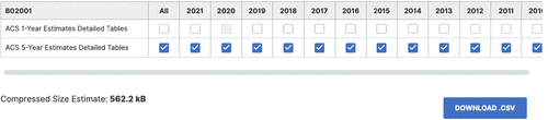
Before proceeding, you can either use our 2020 file or you can download your own, which potentially could be different.
[
Using pandas and the read_csv functionality, read the data set, using as a header the second row (i.e., in Python terms, header = 1) [O1].
For every zip code that has a population higher than 0 (i.e., the “Estimate!!Total:” column should have a value that is greater than zero), calculate two fractions:
• Fraction of the population identifying as white only vs. the total population. You may need to access the data in the “Estimate!!Total:!!White alone” column [O2].
• Fraction of the population identifying as black or African American only versus the total population. You may need to access the data in the “Estimate!!Total:!!Black or African American alone” column [O2].
For every zip code, categorize it as majority white or majority black. This will be necessary in formulating our hypothesis test [O1, O2].
Ameenah identifies herself as Black. Hence, she would like to focus her research on these zip codes (including her own community, which so happens to be categorized as majority black).
At this point, in the next part, we will contrast tickets sent to majority White or majority Black zip codes in Illinois. Of course, we could have investigated tickets sent to majority Latino or American Indian or Alaskan Native, and so on. We leave these analyses as a possible extension to the interested student.
2.4. Hypothesis Testing
We now proceed with the formulation of our statistical hypothesis. Going back to the title of Section 2, we ask ourselves: “are red light cameras racist?” In mathematical terms, is the number of tickets sent to majority black household ZIP codes larger than the number of tickets sent to majority white household ZIP codes?
[
Formulate a suitable statistical hypothesis to test whether majority black ZIP codes receive more tickets than majority white ZIP codes [O3].
Establish the limits of rejection for [O4].
For this next part, you will need to use the information you have collected from Exercises 1–3.
Using the data from Exercises 1–3, do we have enough evidence to believe that majority black ZIP codes receive more tickets from automated camera systems than majority white ZIP codes [O3]?
What is the p value [O4]?
2.5. Conclusion
In lieu of a conclusion, we ask you to continue the discussion with the rest of the members in your group. How does hypothesis testing help as a tool for policy and social change?
[
Another reason why this is happening lies in the criteria of the selection of the intersections. Per your observations and results, specific drivers are more burdened than others from red light cameras and other automated traffic law enforcement mechanisms. If indeed the locations of these mechanisms are selected because they are unsafe, this speaks volumes for the lack of high-quality transportation infrastructure near cities and neighborhoods that are majority minority. Conversely, if the locations are selected with less transparent methods (and indeed, most red light cameras are located in intersections that are deemed as safe by the Illinois Department of Transportation; Mahr and Walberg 2017), then this lack of transparency can lead to the unfair ticket allocation we have been observing.
Now, imagine living in one of the areas that have been consistently ticketed from these automated traffic cameras and law enforcement mechanisms, like Ameenah. Getting ticketed could lead to financial ruin (Sanchez and Kambhampati 2018), so you opt for the next best thing: avoiding these “red zones” on your next commute, adding precious time to your drive and leading you to loss of opportunities. How about we investigate this next? Also, why don’t we help Ameenah figure out how much more time she would need to spend driving for her job to avoid getting ticketed as much?
3. Price of Unjustness
Here, we focus on an optimization problem: specifically, we discuss the shortest path problem on networks. Let G(V, E) be a transportation network, where V represents the set of all intersections (nodes) and E the set of all streets (edges). Associated with every street we have a travel time parameter, which is the amount of time it takes to traverse that street. A driver beginning their trip from an origin node (source s) and ending their trip to a destination node (terminal t) is expected to solve a shortest path problem to minimize their travel time. As an example, we present the transportation network of Figure 3.
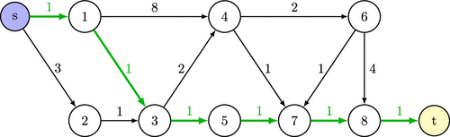
Note. The total travel time/cost is 6 units.
3.1. Defining the Optimization Problem
Now, based on our earlier discussion, people may opt to avoid certain intersections due to their being red zones. Let us locate some red zones in our toy network from Figure 3 and see what happens when trying to solve the shortest path problem while avoiding all red zones.
In Figure 4, we show the optimal solution to the shortest path connecting s to t while avoiding the one red zone in the network. That said, in most real-life transportation networks, there will be more than one red zone to avoid: We show such an example in Figure 5.
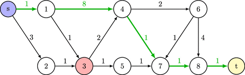
Note. The travel time/cost has now increased to 12 units.
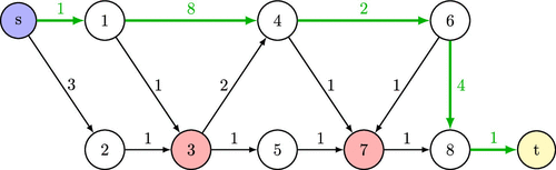
Note. The travel cost has further increased to 16 units, more than double the one of the unrestricted shortest path of Figure 3.
[
This would be the problem that Ameenah would solve under regular circumstances. As a matter of fact, when using her phone to get directions for her next stop, she does choose the fastest route. Let us contrast that to the next optimization problem.
[
This sounds extreme to Ameenah, but at least she would be certain not to have these extra ticket costs! However, is it unfair that she has to go through all these restrictions just to be safe from automated traffic law enforcement tickets: no? We quantify this next.
[
3.2. Incorporating a “Risk Budget”
As you may have observed, and as Ameenah already noted earlier, it may be unrealistic or even outright impossible for a driver to be able to indeed avoid all red zones. Instead, we may expect a driver to try to pass from few of them in their commute. Let us define a parameter as a risk budget: their allowance of how many red zones they are willing to risk driving through during their travel. As an example, consider the solution shown in Figure 6, where the driver has a budget and hence are allowed to drive through at most one red zone during their trip from s to t.
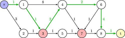
Notes. The driver has a budget of , meaning they are willing to take the chance of driving through at most one red zone. Observe that this flexibility allows them a faster shortest path than in Figure 5: Their shortest path now has a total travel time/cost equal to 11 units.
[
Ameenah can see herself use that “risk budget” idea in her daily routing plan. She can also incorporate other criteria (how much time she has until her next stop, how important the next stop is, and whether she has a time window or deadline, etc.) in her decision-making process. For example, she may opt to pass through fewer (or zero) red zones if she has more flexibility until she gets to her next stop. However, she may need to take her chances and solve the unrestricted shortest path version (that is, allowing for any “red zones”) if she is on a tighter schedule.
Now, let us rework this, focusing on the Chicago, Illinois, transportation network. We have used osmnx (Boeing 2017) to obtain the transportation network of the city using a filter to isolate all primary, secondary, tertiary, and residential links in the area. We do so through the following set of Python statements.
We selected speed limits for the streets in the network: This way, we may use the ox.add_edge_travel_times(G) statement to obtain travel times on a street level. These times do not account for any traffic that, as we may already know, can be quite significant in Chicago. Finally, the full network with the travel times is given to use in the provided chicago.txt file. In Figure 7 (left), we provide the plotted Chicago, Illinois, transportation network.
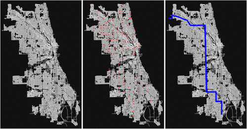
Notes. Drive network of Chicago, Illinois, obtained using osmnx is shown on the left. In the center, the same map with the red zones identified using the locations of all traffic cameras. Finally, on the right, we reveal the actual shortest from South Chicago to O’Hare International Airport (ORD).
Using your mathematical formulation and your code from Exercise 6 for solving the simple, unrestricted shortest path problem, report the amount of time it would take a person to drive from South Chicago (node: 261276337 corresponding to coordinates of -87.622000, 41.684301) to O’Hare International Airport–ORD (node: 261341174, corresponding to coordinates of −87.904724, 41.97861) [O6]. We reveal the solution on the map in the rightmost image of Figure 7.
We now move to our last part, the one that shows the price of unjustness for drivers who will try to avoid red zones, for good reason. The cost of a red light traffic camera ticket in Chicago, Illinois, is $100 if traveling with 11 miles per hour over the speed limit and $35 if traveling with 6–10 miles per hour over the speed limit. The fine doubles if not paid within 25 days. At the same time, traveling delays incur a cost for the drivers. Empirical studies (Liu et al. 2007) demonstrate that the value of travel time can vary from $5 to $30, whereas costs associated with travel time uncertainty materialize in the form of scheduling costs and are 30%–40% of the generalized costs (Ettema and Timmermans 2006).
To help you in the next activities, we provide you with a file named cameras.txt containing all locations for automated traffic camera ticketing systems (i.e., red zones). These are also visualized in Figure 7 (right) for convenience: The locations are marked in red.
[
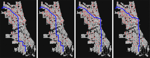
Note. Equivalently, these are the shortest paths with risk budgets .
3.3. Conclusion
Instead of a conclusion, we again ask you to have a discussion with your peers on your results. What do you observe as the budget of a person (their willingness to risk driving through a red zone) decreases?
[
How much tougher does the path get? We can define the difficulty of following a path as the number of “zig-zags” or turns the driver needs to take [O7].
Knowing that many higher speed streets are outside the downtown area of Chicago, what do you observe about driving through the downtown area of Chicago as the budget decreases? If unfamiliar with the Chicago area, consult an online map (such as Google or Apple maps) to identify the downtown area [O7].
1 Adapted from the story of Rodney Perry in the original ProPublica article (Sanchez and Kambhampati 2018).
References
- (2017) Osmnx: New methods for acquiring, constructing, analyzing, and visualizing complex street networks. Comput. Environment. Urban Systems 65:126–139.Crossref, Google Scholar
Centers for Disease Control and Prevention (2022) Automated red light camera enforcement. Accessed March 1, 2023, https://www.cdc.gov/transportationsafety/calculator/factsheet/redlight.html.Google Scholar- (2006) Costs of travel time uncertainty and benefits of travel time information: Conceptual model and numerical examples. Transportation Res. Part C Emerging Tech. 14(5):335–350.Crossref, Google Scholar
- (2015) Countermeasures that work: A highway safety countermeasure guide for state highway safety offices, 2015. Technical report, Department of Transportation, National Highway Traffic Safety, Washington, DC.Google Scholar
- (2022) Chicago’s “race-neutral” traffic cameras ticket black and latino drivers the most. ProPublica (January 11), https://www.propublica.org/article/chicagos-race-neutral-traffic-cameras-ticket-black-and-latino-drivers-the-most.Google Scholar
Insurance Institute for Highway Safety (IIHS) (2023) Red light running: Red light camera communities. Accessed October 1, 2023, https://www.iihs.org/topics/red-light-running/red-light-camera-communities.Google Scholar- (2007) Estimation of the time-dependency of values of travel time and its reliability from loop detector data. Transportation Res. Part B: Methodological 41(4):448–461.Crossref, Google Scholar
- (2017) Tribune investigation: IDOT approves red light cameras for already safe intersections. Chicago Tribune (September 23), https://www.chicagotribune.com/investigations/ct-idot-red-light-cameras-met-20170921-story.html.Google Scholar
- (2018) How Chicago ticket debt sends black motorists into bankruptcy. ProPublica (February 27), https://features.propublica.org/driven-into-debt/chicago-ticket-debt-bankruptcy/.Google Scholar