


The Snake Eggs Puzzle: Preparing Students for Benders Decomposition
Abstract
Logic puzzles are an effective way to introduce students to advanced solution techniques in operations research, such as Lagrangian relaxation, Dantzig-Wolfe decomposition, and Benders decomposition. The Snake Egg puzzle asks the player to draw a one-cell wide path, or “snake,” in a grid. The remaining cells should form a fixed number of separate, connected, discontiguous regions called “eggs.” We propose two solution approaches: a flow-based model and lazy constraints. Instead of providing the complete model at the outset, we will step through the puzzle in a manner suitable to the classroom, emphasizing the skills that are crucial to successfully implementing advanced techniques. The puzzle functions in particular as a prelude to Benders decomposition.
Funding: M. Harris is supported by an Australian Government RTP (research training program) scholarship.
1. Introduction
Logic puzzles are an effective way to teach modeling techniques in operations research, because many puzzles can be formulated as integer programs (IPs). Sudoku, for instance, is now a classical teaching example; see Conforti et al. (2014). Chlond (2015a) formulated an IP model of a chess avoidance puzzle. Chlond (2015b) formulated IP models of the Wijuko and ABC logic puzzles. Hartmann (2018) formulated IP models of several popular mobile puzzles. Many other examples can be found in this journal. But besides providing many IP modeling examples, logic puzzles are also an opportunity to demonstrate the kind of speedups that can be achieved by using advanced operations research techniques, such as Lagrangian relaxation, Dantzig-Wolfe decomposition, and, of most interest to us, Benders decomposition. For example, Pearce and Forbes (2017) proposed both row and column generation approaches to the so-called fillomino puzzle, which is difficult to solve by a direct approach.
Benders decomposition is a method of solving certain difficult optimization problems, where new constraints are added to a master problem in each iteration; see Benders (1962). Row generation algorithms like this have historically been implemented either in a loop, where the master problem is solved from scratch in each iteration, or by a specialized branch-and-cut procedure. Since 2012, however, modern solvers such as Gurobi (Gurobi Optimization LLC 2022) have included lazy constraints, allowing us to easily add user cuts at nodes of a branch-and-bound tree.
Lazy constraints, unlike valid inequalities, are allowed to cut off feasible solutions to the base model. In that way, they can be used to enforce properties that have been left out of the full model. A classic example is the Dantzig-Fulkerson-Johnson formulation of the traveling salesman problem. Although the exact formulation has exponentially many subtour elimination constraints, by adding only the ones that are violated by incumbent solutions to the relaxed problem, we can solve even relatively large instances in a reasonable amount of time; see Dantzig et al. (1954).
Teaching experience indicates that Benders decomposition is a nontrivial conceptual step above the standard linear and integer programming techniques covered during a first course in operations research. Thus, it is beneficial to introduce some of the basic notions with a logic puzzle before covering the correctness proof or any industrial applications. In this paper we will study the Snake Egg puzzle. The puzzle is credited to Serkan Yürekli and (at this time) can be found at https://www.gmpuzzles.com/blog/2016/01/snake-egg-by-serkan-yurekli/.
After stating the puzzle, we will try to formulate it as an integer program, visualizing the new solution each time new constraints are formulated. In doing so, we stress the value of incremental modelling and the types of early end-to-end testing techniques that are crucial for successfully implementing an advanced technique.
One of the puzzle rules—the connectivity of the snake eggs—turns out to be the most challenging part. We consider two approaches to enforcing this rule: a multicommodity flow approach and lazy constraints. Although enforcing connectivity is an interesting use of flow-based constraints, we find the lazy approach to be superior with respect to runtime. We also demonstrate some useful techniques and principles for benchmarking various approaches to a problem.
After solving the snake egg puzzle, students can meet Benders decomposition familiar with several important concepts, such as omitting the complicating aspects of a problem, adding new constraints at nodes of the branch-and-bound tree, the importance of strong cutting planes, and disaggregated cuts.
1.1. The Snake Egg Puzzle
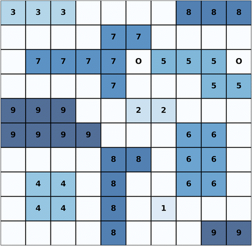
The Snake Egg puzzle is played on a grid of cells. We want to draw a snake—that is, a one-cell wide path moving orthogonally—in the grid. The head and tail of the snake are fixed and labeled with an “O” in our figures. The snake may not touch itself orthogonally. The remaining cells should form a fixed number of separate, connected, discontiguous regions—or eggs—of sizes , etc., up to the specified number of eggs. The value of some cells may be fixed in advance. We consider two instances: a 6 × 6 instance with five eggs and the 10 × 10 instance with nine eggs from the aforementioned blog post (see Figure 1).

2. Formulation
The puzzle is characterized by the following sets and data (Table 1).
|

Table 1. Notation
| Sets | Descriptions |
|---|---|
| S | The set of cells |
| The set of cells adjacent to cell | |
| The set of egg sizes | |
| The set of cell types | |
| The set of cells with predetermined values | |
| The predetermined value of cell |
To formulate the puzzle as an integer program, we need to determine a suitable set of variables. Because we want to associate each cell with an integer k, it is tempting to try and use general integer variables. But this will make it difficult to write down the constraints. Instead, we define binary variables, for and , with the following interpretation:
Here, means that cell s is part of the snake. In our visualizations, we leave snake tiles blank, except for the head and tail.
Using binary variables—which are more numerous—may contradict the instinct to minimize the number of integer variables when possible. But modern IP solvers are very good at exploiting the geometry of the unit hypercube for the generation of cutting planes, when making branching decisions, in pre-solve, and in other contexts.
Several constraints are now obvious:
Each cell belongs to exactly one egg or the snake:
(1)There are k cells in egg k for :
(2)The values of preset cells are fixed:
(3)
We can solve (1–3) to get a starting visualization that helps to prompt other constraints; see Figure 2.
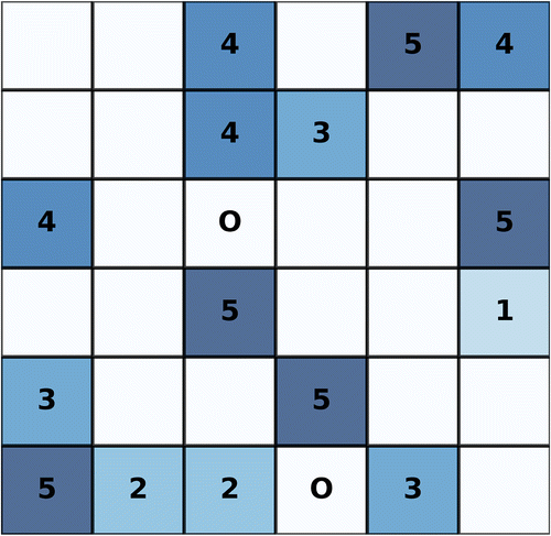
Although the eggs are the right size, they have been scrambled. We want to pull together the cells of similar type. A start is to observe that each cell of type should have at least one neighbor with the same egg type. We can impose this with
After re-solving the model, we get the solution in Figure 3.
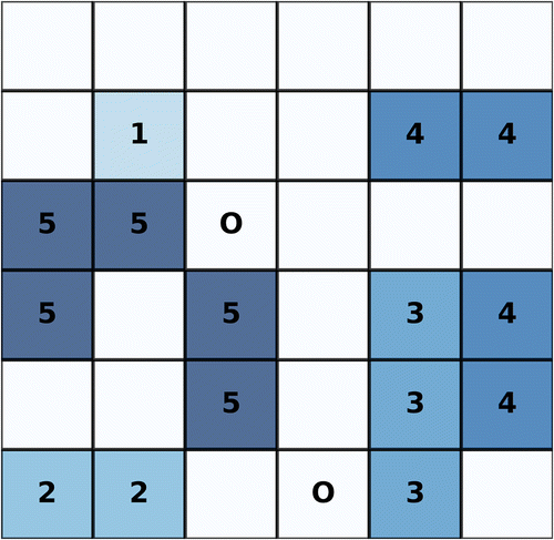
This is closer to a valid solution, but different eggs can still touch. To push the eggs apart we impose
Now if cell s is a part of egg k, then each cell is part of k as well, or it is part of the snake. Solving the model again gives the solution in Figure 4.
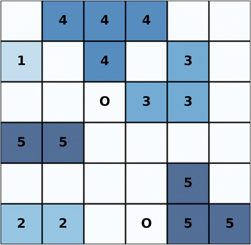
There are two more obvious problems; the egg is disconnected, and the snake is not actually a snake. We know that the head and tail of the snake need to be adjacent to exactly one other snake cell each:
This gives the solution in Figure 5. Next, each interior cell of the snake should be adjacent to exactly two other snake cells. A common suggestion from students is
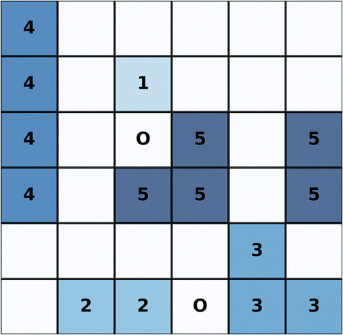
This works if . But if , then it prohibits any neighbor of s from being a snake cell, leading to an infeasible model. Instead, we add two sets of constraints:
If , then together these constraints imply , as required. But when , we get , which is vacuous. Re-solving the model now gives the solution in Figure 6.
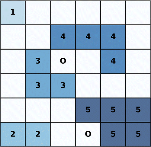
This is a valid solution to the 5 × 5 instance. But an astute student will notice that the and eggs are connected only by coincidence. In general, (4) is sufficient only for the and eggs. This becomes clear when we try to solve the 10 × 10 instance. See Figure 7, where the and eggs are disconnected and there is a separate loop in the snake. We will consider two approaches to enforcing connectedness and eliminating loops.
2.1. Flow Formulation
We can enforce the continuity of the snake eggs and the snake by imposing a multicommodity flow superstructure. The idea is to choose an arbitrary source for each egg and the snake. Each other cell in each egg receives one unit of flow from its source. Flow conservation then guarantees that the cells are connected.
For each and , let ysk be a binary variable with the following interpretation:
For , and , let be a continuous variable with the following interpretation:
We make sure there is only one source per egg, including the snake, with
We guarantee that only a type k cell can be the source for egg k with
For , we limit the outflow of each cell to k – 1 if that cell is the source of commodity k, to k – 2 if it is a type k cell, but not a source, and to zero otherwise with
We enforce flow conservation for the eggs with
In other words, if cell s is the source for commodity k, then the net outflow is k – 1. Otherwise, the net inflow is 1. Finally, we enforce flow conservation for the snake with
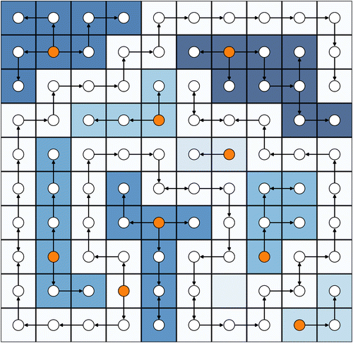
Note that retaining (4) means no flows of commodities 2 and 3 are needed. We could also fix the source of the snake flow to one of the ends. Constraints (1–13) constitute a compact formulation of the snake egg puzzle, because the number of variables and constraints is polynomial in the size of the puzzle.
3. Lazy Constraints
Although the flow formulation of the 10 × 10 puzzle is not intractable, we can speed up the solution time by using lazy constraints. In this section, we drop the flow variables and constraints (9–13). We will call (1–8) the master problem. One way to solve the Snake Egg puzzle is to solve the master problem over and over again in a loop, where in each iteration we check whether the eggs are connected. If they are not, we add a new constraint that bans that solution and continue. Say that is the incumbent solution. One such constraint is
The question to ask ourselves is as follows: Given the current master solution, can we come up with a stronger constraint that not only cuts off the current solution but also a large number of other bad solutions at the same time, a good cut, so to speak? Say that C is a disconnected subset of the egg in the current solution. The no-good cut can be satisfied by exchanging the value of any two cells in while preserving the disconnected egg. But because and the eggs must be connected, we know that region C can only be part of egg k if at least one cell directly adjacent to C is part of the egg as well. Let’s make this formal.
For , define to be the set of all subsets with such that C is connected. For , let
In other words, for and , the set C may not be a subset of egg k unless at least one neighbor of C is, too. Now (1–8, 14) is an exact formulation of the Snake Egg puzzle. A formal proof of this fact is in the Appendix.
Unlike the flow model, this is a noncompact formulation, because (14) is an exponential number of constraints. Therefore, adding them all to the model is not an option. Instead, we can solve the master problem and, at nodes of the branch-and-bound tree, use special-purpose code to detect the disconnected eggs. For each connected component of a disconnected egg, we add the corresponding constraint from (14) as a lazy constraint and continue with the solve. The hope is that significantly fewer constraints will be needed before we discover a good solution.
It turns out that we can do even better by disaggregating the cuts. The following family of constraints also guarantees that all eggs are contiguous:
A formal proof of this, too, may be found in the Appendix. The constraints state that each individual cell in the disconnected region is deactivated unless at least one more cell on its boundary has the same type. Note that the “aggregated” cuts are obtained by summing the disaggregated cuts over . We will add each cut as a separate lazy constraint, as required.
3.1. Results
Integer programming solvers are well-known to be chaotic systems; runtimes can vary dramatically with the path taken through the branch-and-bound tree. This is even more pronounced with feasibility problems, where with good luck we could stumble upon a solution very quickly. Therefore, to do rigorous benchmarking, we need to test the proposed approaches on many instances. We would like to compare the following approaches to the 10 × 10 puzzle:
Solving once with (15) added as lazy constraints; Lazy
Solving from scratch in each iteration, with (15) added as regular constraints; Loop,
; Flow.
We solved the 10 × 10 instance 1,000 times for each approach using distinct seeds, which impact the path taken through the tree. The models were programmed in Python 3.8.12 via the Anaconda distribution (4.11.0) and solved using Gurobi 9.1.2 (Gurobi Optimization LLC 2022). Jobs were run in parallel on a computing cluster operating 2.5 GHz CPUs. Each job was given a time limit of 10 minutes and a single thread. Performance profiles can be found in Figure 9.
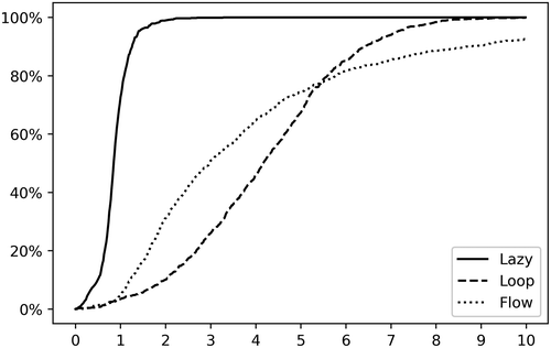
The horizontal axis represents time in minutes. The vertical axis represents the percentage of 1,000 instances solved within that time. Although some of the fastest runs of the flow model outperform the slowest runs of the lazy model, the general trend is clear. The lazy model solves all instances within 3 minutes, and many of them much faster than that. On the other hand, the flow model fails to solve some instances even within 10 minutes. The intersection of the Loop and Flow curves is also interesting. Minimum, maximum, mean, and standard deviations of the runtimes are given in Table 2; note that the Flow column is skewed in its own favor because 68 instances timed out before finding a solution.
|
Table 2. Comparing Three Formulations
| Time (s) | Lazy | Loop | Flow |
|---|---|---|---|
| Minimum | 0.37 | 0.39 | 7.9 |
| Maximum | 196.32 | 585.92 | 616.79 |
| Mean | 52.19 | 250.56 | 202.37 |
| SD | 20.62 | 103.31 | 129.89 |
3.2. Improvements
Students often suggest improvements to the model in class. In this section, we outline two of these suggestions.
Let be the set of all 2 × 2 connected squares of the form
Then,
A second suggestion from students came before the lazy constraints had been introduced. Having asked the students to think of ways to enforce the connectivity of the snake eggs, one suggestion was to introduce an objective function maximizing the number of connections between adjacent egg cells. Although a novel and very reasonable suggestion, we were able to confirm that it does not produce a valid solution to the puzzle; the optimal solution includes a disconnected loop in the snake. What we can do is incorporate the objective function into the lazy model and simply terminate when a valid solution is found. The hope is that the objective will encourage the solver to favor connected eggs.
Figure 10 contains performance profiles for the standard lazy model, the lazy model with an objective function, and the lazy model with the valid inequalities.
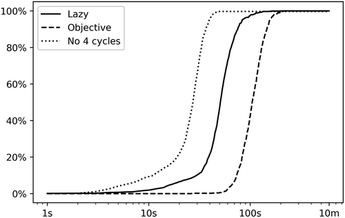
This time we have plotted the profiles on a logarithmic scale. We see that including an objective function actually hinders the model. On the other hand, the valid inequalities approximately halved the runtime. See the table of results (Table 3).
|
Table 3. Comparing Two Potential Improvements
| Time (s) | Lazy | No-4 | Obj. |
|---|---|---|---|
| Minimum | 0.37 | 1.25 | 26.98 |
| Maximum | 196.32 | 49.1 | 218.93 |
| Mean | 52.19 | 25.7 | 107.84 |
| Dev | 20.62 | 9.4 | 28.52 |
4. Conclusion
In this paper, we have shown how up to a 10 × 10 instance of the Snake Egg puzzle with nine eggs can be solved using lazy constraints. Instead of providing the complete model at the outset, we stepped through the puzzle in a manner suitable to the classroom. Advantages of this include (i) the early detection of errors and (ii) early visualization of partial solutions. We benchmarked several approaches and found the lazy approach to be superior with respect to runtime. The lazy approach we have described is, in fact, an example of so-called Logic-Based Benders decomposition; see Hooker (2000) and Hooker and Ottosson (2003). In that context, the lazy constraints are called feasibility cuts. We believe that the snake egg puzzle is an effective pedagogical prelude to both classical and logic-based Benders decomposition.
We thank the editors, reviewers, and all involved for their consideration of our work.
Appendix. Correctness of the Lazy Constraints
Fix and an integer solution to (1–8), and let . Then, satisfies every constraint of (14) indexed by k if and only if C is connected.
) Suppose C is connected. Choose . If , then
If , then
Because was arbitrary, every constraint in (14) indexed by k is satisfied by .
) Conversely, suppose C is not connected. Without loss of generality, there exists and with and . Therefore,
Fix and an integer solution to (1–8), and let . Then, for satisfies every constraint of (15) indexed by k and s if and only if C is connected.
) Suppose C is connected. Choose and . If , then
If , then
Because and s were arbitrary, satisfies every constraint in (15).
) Suppose C is not connected. Without loss of generality, there exists and with and . Therefore, for each ,
References
- (1962) Partitioning procedures for solving mixed-variables programming problems. Numerische Mathematik 4:238–252.Crossref, Google Scholar
- (2015a) Puzzle—chess avoidance puzzles. Trans. Educ. 15(3):254–256.Link, Google Scholar
- (2015b) Puzzle—ip in the i. Trans. Educ. 16(1):39–41.Link, Google Scholar
- (2014) Integer Programming, volume 271. (Springer). https://link.springer.com/book/10.1007/978-3-319-11008-0.Crossref, Google Scholar
- (1954) Solution of a large-scale traveling-salesman problem. J. Oper. Res. Soc. Am. 2(4):393–410.Link, Google Scholar
- (2022) Gurobi Optimizer Reference Manual. https://www.gurobi.com.Google Scholar
- (2018) Puzzle-solving smartphone puzzle apps by mathematical programming. Trans. Educ. 18(2):127–141.Link, Google Scholar
- (2000) Logic-based Methods for Optimization: Combining Optimization and Constraint Satisfaction. (Wiley, New York).Crossref, Google Scholar
- (2003) Logic-based benders decomposition. Math. Programming 96(1):33–60.Crossref, Google Scholar
- (2017) Puzzle-the fillomino puzzle. Trans. Educ. 17(2):85–89.Link, Google Scholar

