Case—AdWords to AdWards: Online Optimization for Hospital Patient Placement
Abstract
This case illustrates online optimization algorithms for sequential decision making. Students are asked to translate an unfamiliar healthcare setting into a well-known online optimization problem, the Google AdWords problem. The case is based on an actual process improvement project aimed at maximizing the use of a hospital’s capacity. The main character, Dr. Kelly, heads an observation unit and had tried a predictive model for patient assignments to her unit versus the hospital wards, which, however, can sometimes lead to inefficient bed capacity management. She is looking to improve patient allocation decisions made in real time. The complexity of the healthcare environment makes the mapping challenging, requires discussions with experts with domain knowledge and various stakeholders in the process, and raises ethical questions.
Dr. Kelly’s Dilemma
Dr. Erin Kelly was in charge of a 23-bed observation unit at Montanaro, a 260-bed hospital in a medium-sized U.S. city. Observation units (OUs) house observation status patients with complex but not life-threatening symptoms so that healthcare providers can observe such patients for a period of time and decide whether inpatient hospitalization is required or whether the patient can be safely discharged from the hospital. In practice, not all observation status patients are placed in the OU, which has a limited capacity; some are placed directly in the inpatient wards. Patients placed in the OU are expected to spend, on average, 48 hours before being moved to the wards or discharged.
After analyzing data from the OU several months ago, Dr. Kelly had become concerned about the long length of stay (LOS) for some OU patients, as well as the high percentage of OU patients who “flipped,” or acquired inpatient status, while in the OU. The former group of patients took up space in the OU that could be assigned to patients who could benefit more from the OU beds. The latter group of patients spent a lot of time in transit between departments at the hospital. Dr. Kelly focused on patients placed in her OU after presenting at the emergency department (ED) and collaborated with a professor at a nearby university, Professor Viviana Devis, to build predictive models to identify patients who were likely to flip after being placed in the OU. Such patients could be placed directly in the inpatient wards after presentation at the ED. Appendix A contains the data dictionary for the data set Dr. Kelly and Professor Devis used in the original analysis (Table A.1), as well as an example of what the final predictive model could have looked like (Figure A.1).
Decisions in healthcare settings are never easy or clear-cut. Predictions of the likelihood that a patient would flip were not perfect, and many patients were borderline cases, so they could be considered for both OU and inpatient ward placement. In addition, when testing the recommendations of the predictive model on past patient arrival data, Dr. Kelly and Professor Devis observed that sometimes the OU would not be very busy while the inpatient wards would be full, and vice versa. Dr. Kelly wanted to know when she could take in more patients to help congestion in the inpatient wards and when she should save capacity in the OU.
Dr. Kelly reached out to Professor Devis once again. Professor Devis had been working on online optimization algorithms for ad placement and order fulfillment. The description of Dr. Kelly’s problem reminded her of such settings. She wondered whether online optimization algorithms could be used to address Dr. Kelly’s question.
Sequential Decision Making and Online Optimization
Offline optimization algorithms are built on the assumption that all necessary data are available beforehand, allowing for decisions to be made after analyzing the entire data set and enabling careful planning to achieve the optimal solution. There are settings where this is an appropriate approach; typically, such settings have a static environment where conditions remain relatively stable over time and do not require an immediate response. Many decisions in the real world, however, must be made in a dynamic environment where conditions change rapidly and unpredictably. The person or system issuing a request requires a response immediately; it is not feasible to wait for additional information to arrive before deciding how to serve the request in the most cost-efficient or profit-maximizing way. Such situations call for real-time (also referred to as online) decision making in which decisions are made sequentially as new data become available. Examples of such settings include sales of different fare classes of airline tickets, online advertising, dynamic pricing, and inventory management for new products.
An Illustrative Example
A classic example of the online decision-making setting is the so-called “AdWords problem” that arises in online advertising. The goal is for an online advertising platform to allocate a sequence of advertising spaces associated with search queries to budget-constrained advertisers in a way that maximizes the platform’s expected revenue. This problem is an example of online matching problems, studied extensively in computer science.
Let’s consider a particular instance of the AdWords problem (Figure 1). Suppose there are advertisers (bidders), , with specified budgets . is a set of query words . Each advertiser specifies a bid for query word . If advertiser s ad is shown when query word arrives, the platform realizes the revenue from the bid only if the customer who generated the query clicks on the ad. Assume that the click-through rate for s ad for query word is approximately known based on past data. This means that the expected revenue to the platform from showing s ad for query word can be estimated as .
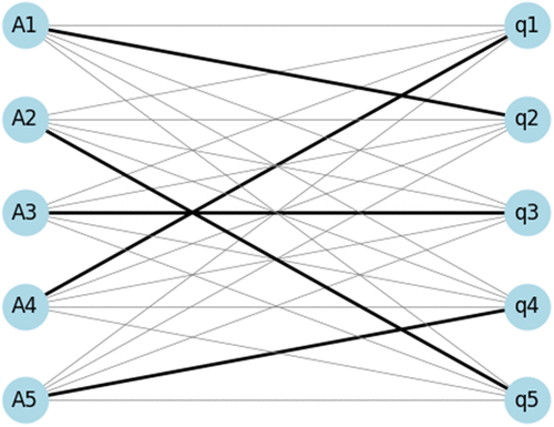
Note. Advertisers (nodes on the left) need to be matched with arriving queries over time (nodes on the right).
A sequence of query words arrive during the day, where denotes the type of the th word that arrives. Suppose that there is a single ad slot and each query must be assigned to an advertiser . Which advertiser should be selected?
The “Clairvoyant” Problem
If the sequence of query words were known in advance, the problem could be solved as follows. Consider decision variables if query word arriving at time is allocated to advertiser , and zero otherwise. (The subscript here is only used to denote the different query word arrivals. The relative ordering of and the exact time at which queries arrive do not matter.) We can formulate the following offline optimization problem:
Maximize
This formulation is referred to as the “clairvoyant” problem because the resulting allocations are created assuming that future arrivals are known, and therefore, they are the best they can be. If all information is known in advance (i.e., we know what the query type of each arriving query will be over the time horizon ), the optimal allocation across all arriving queries and all advertisers over given their budgets can be found. A simple example is described in Appendix B.
Heuristics
Unfortunately, the types of queries arriving over time are not known in advance, and decisions need to be made in an online fashion. Heuristics—quick methods to arrive at decisions that “make sense” but are not guaranteed to be optimal—can be employed in such circumstances; however, some heuristics are better than others. A purely “greedy” heuristic—one that allocates each arriving query to the advertiser with the highest bid for that query until the advertiser’s budget is exhausted—may seem logical, but it often performs poorly in practice.
What Constitutes “Good” Performance for an Online Algorithm?
The performance of an online algorithm is often evaluated through the competitive ratio: the ratio of the worst-case value obtained by the online algorithm (revenue in the case in the AdWords problem) over the sequence of arrivals and the best value achievable by the offline clairvoyant algorithm. How do we know the best value achievable by the offline clairvoyant algorithm if we do not know the sequence of arrivals in advance? We can sometimes calculate a bound for it. An online algorithm is said to be -competitive if, for every instance, the ratio of the revenue of the online algorithm to the revenue of the best offline algorithm is at least .
An important breakthrough in developing online algorithms for online matching problems (and the AdWords problem in particular) was the realization that instead of a purely greedy algorithm that assigns queries to advertisers based on the magnitude of their bids, one can calculate “rewards” that represent the bids scaled to reflect the remainder of the advertisers’ budgets at that point in time and use those rewards for allocation purposes. Having observed a query and calculated the rewards for each query-advertiser pair, the online algorithm would allocate the current query to the advertiser with the highest reward (rather than the highest bid ). An advertiser whose budget is almost exhausted (i.e., the ratio is very small) would have its bid scaled down, reducing the reward of allocating the current query to that advertiser relative to other advertisers with comparable bids but whose budgets have not been exhausted yet.
The reward of allocating query to advertiser with bid , initial budget , and current (remaining) budget is defined as
Selecting an exponential function instead, , results in a greater penalty the first time an advertiser’s budget is used but then less dramatic further penalties for depleting the budget; see Figure 2. In practice, this exponential function is often scaled by a factor of , which keeps it in the range and ensures more balanced penalties as the budget is decreased. The reward for the scaled exponential function is determined as
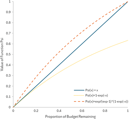
The choice of affects the performance of the online optimization algorithm. In particular, using the exponential function has been shown to result in a good competitive ratio of under certain conditions. The exact definition of the function is sometimes guided by the so-called “dual” problem of the “primal” clairvoyant optimization problem. The dual variables corresponding to the constraints in the primal problem are used to assess the incremental value of depleting a particular budget or resource. Such primal-dual approaches have been successfully applied, for example, by online retailers when deciding from which warehouse orders should be shipped to customers given shipping costs and available inventories or to determine personalized assortments to offer to customers given limited inventories of the products used in the assortments.
Appendix B describes further the difference between the greedy and the “scaled greedy” online algorithms for simple examples, and shows how one could calculate the competitive ratio.
Online Capacity Balancing for Montanaro?
Professor Devis reviewed the summary data provided by Dr. Kelly. (See Table 1 and file OUSummaryData.xlsx.) Use this information to address the following questions:
|

Table 1. Summary Data from Dr. Kelly’s Data Set
| DRG code | Description | Percentage | Probability of flipping | Expected LOS, OU start | Expected LOS, W start | Difference W-OU LOS |
|---|---|---|---|---|---|---|
| 276 | Dehydration | 0.1175 | 0.6033 | 5.71 | 6.73 | 1.01 |
| 428 | Congestive heart failure | 0.0438 | 0.6122 | 3.75 | 5.76 | 2.02 |
| 486 | Pneumonia | 0.0569 | 0.5789 | 3.44 | 5.46 | 2.02 |
| 558 | Colitis | 0.0336 | 0.7273 | 5.71 | 3.69 | −2.02 |
| 577 | Pancreatitis | 0.0187 | 0.7619 | 3.42 | 3.42 | 0.00 |
| 578 | GI bleeding | 0.0392 | 0.5366 | 5.47 | 8.50 | 3.03 |
| 599 | Urinary tract infection | 0.0765 | 0.6585 | 7.99 | 5.97 | −2.02 |
| 780 | Syncope | 0.2761 | 0.3725 | 5.68 | 9.72 | 4.04 |
| 782 | Edema | 0.0196 | 0.3913 | 4.80 | 3.79 | −1.01 |
| 786 | Chest pain | 0.1371 | 0.3378 | 3.20 | 9.26 | 6.06 |
| 787 | Nausea | 0.0793 | 0.4578 | 3.33 | 7.37 | 4.04 |
| 789 | Abdominal pain | 0.1017 | 0.3287 | 3.66 | 6.69 | 3.03 |
Note. The columns in the table show the 12 most frequently encountered diagnoses in the ED (“DRG code” column), the definition of the diagnosis (“Description” column), the average percentage of cases for each diagnosis (“Percentage” column), the probability of flipping for each diagnosis, the expected length of stay (LOS) when the patient starts in the OU vs. the wards (“Expected LOS, OU start” and “Expected LOS, W start” columns, respectively), and the difference between the two expected LOS (“Difference W-OU LOS”).
Can Dr. Kelly’s problem be represented as an online optimization problem similar to the AdWords problem? If yes, what would be the equivalent for the advertisers, budgets, bids, click-through rates, queries, and query types in Dr. Kelly’s problem?
What could constitute a “revenue” associated with matching a query with an advertiser in Dr. Kelly’s context?
Appendix A. Predictive Model Information
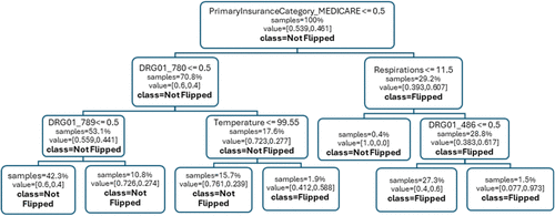
|
Table A.1. A List of Variables and Their Definitions Used by Dr. Kelly and Professor Devis to Build the Predictive Model
| Variable | Definition |
|---|---|
| Age | Age of patient, in years |
| Gender | Patient gender (recorded as male/female) |
| PrimaryInsuranceCategory | Insurance provider for the patient, e.g., Medicare, Medicaid, Private, other |
| Flipped? | The value of this variable is “flipped” if a patient flipped from OBSERVATION status to INPATIENT status, and “not flipped” if the patient stayed in OBSERVATION status during the whole stay in the OU |
| OU_LOS_hrs | Length of stay in the OU in hours |
| DRG01 | Primary diagnosis-related group (code) upon admission of the patient in the OU: 276 Dehydration 428 Congestive heart failure 486 Pneumonia 558 Colitis 577 Pancreatitis 578 GI bleeding 599 Urinary tract infection 780 Syncope 782 Edema 786 Chest pain 787 Nausea 789 Abdominal pain |
| BPUpper, BPLower, BPDiff, Pulse, PulseOximetry, Respirations, Temperature | Patient vital signs (BP = blood pressure) |
Appendix B. Simple Examples of Online Algorithms
Let us see some examples of how online optimization algorithms work.
Consider a simple setup in which there are two advertisers, and , with equal starting budgets, and , of two units each. There are two types of query words, and , and the bids advertisers and have placed on those queries are shown in Figure B.1(b). Assume that the click-through rates are always one, and one ad is shown for each arriving query. Suppose that four queries have arrived, the first two of type and the last two of type .
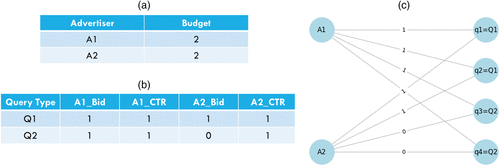
Notes. (a) Advertisers and budgets. (b) Query types, advertiser bids for each query type, and click-through rates. (c) A sketch of the simple example setup.
We next discuss the optimal clairvoyant solution and two “reasonable” algorithms and illustrate the allocations in Figure B.2.
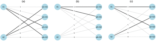
Notes. (a) Optimal clairvoyant solution (revenue = 4). (b) Greedy solution (revenue = 2; competitive ratio = 1/2). (c) Balance-budget solution (revenue = 3; competitive ratio = 3/4).
B.1. Clairvoyant Solution
If we knew in advance that the sequence of query types would be , we would allocate the first two queries, (of type) and (of type), to advertiser , and the last two queries, (of type) and (of type), to advertiser . This would generate the maximum possible revenue of four.
Let’s see how this insight would map to the clairvoyant optimization problem formulation. We know that , , , in advance. We want to find the maximum of the expression for the total revenue in the objective function
We know , , , , and all the click-through rates are one. So, the expression for the total revenue resulting from the allocation is
It is easy to see that the best combination of values for that maximizes the expression for the total revenue is
B.2. Greedy Solution
Under imperfect information about future queries, suppose that we follow a greedy algorithm: assign each arriving query to the advertiser with the highest bid for that query.
The allocation of the four arriving queries from Figure 2(c) will work as follows:
When the first query (of type ) arrives, both ’s and ’s bids are one. (See first row of the table in Figure B.1(b)) We can allocate randomly to one of the two advertisers then. Let’s pick . Revenue so far equals one.
When the second query (of type ) arrives, both and ’s bids are one. (See first row of the table in Figure B.1(b).) Again, let’s allocate randomly to one of the two advertisers, . Cumulative revenue so far equals two.
When the third query (of type ) arrives, ’s bid is one, and ’s bid is zero. (See second row of the table in Figure B.1(b).) If we could, we would allocate the arriving query to ; however, has no budget left. The cumulative revenue therefore remains two.
The situation in query 3 repeats when the fourth query (of type ) arrives.
The total revenue generated by the greedy algorithm is therefore two, and the competitive ratio is 2/4 = 0.50.
B.3. Balance-Budget Solution
Based on the performance of the greedy algorithm, where one advertiser ran out of budget and the other advertiser kept its entire budget but whose ad did not receive any impressions, it seems that it would be important to keep track of the remaining budget of an advertiser. What if, instead of allocating the incoming query to the advertiser with the highest bid, we allocate it to the advertiser with the highest remaining unused budget?
The allocation of the four arriving queries from Figure B.1(c) will work as follows:
When the first query (of type ) arrives, both ’s and ’s budgets are two. We can then allocate randomly to one of the two advertisers. Let’s pick . Revenue so far equals one (’s bid for query type ).
When the second query (of type ) arrives, ’s remaining budget is one,and ’s remaining budget is two. We allocate to given its higher remaining budget. Cumulative revenue so far equals two. (’s bid of one for query type was added to the revenue from step 1.)
When the third query (of type ) arrives, ’s budget is one, and ’s budget is one. We allocate the arriving query to . ’s bid for query of type is one, so the cumulative revenue is now 2 + 1 = 3.
When the third query (of type ) arrives, ’s budget is zero, and ’s budget is one. We allocate the arriving query to . However, ’s bid for query of type is zero, so the cumulative revenue does not increase—it remains at three.
The total revenue generated by the balance-budget algorithm is higher than the total revenue generated by the greedy algorithm (three versus two), and the competitive ratio is better: 3/4 = 0.75.
However, further examples can be constructed to show that (1) taking into consideration not the remaining budget but the percentage of the remaining budget of each advertiser leads to a fairer process (so that smaller advertisers are not ignored), and (2) both the remaining budget percentage and the bid of each advertiser for each keyword should be taken into consideration for better algorithm performance. (In fact, the click-through rate should also be considered, but here we assumed it to be one for all ads.) This is why a calculation for reward of the form
Worksheets AlgLinear and AlgExp in the file OnlineAlgorithmsIllustration.xlsx walk through the calculation with the more sophisticated definition of rewards for linear and exponential function .
Online capacity-balancing algorithms have been studied extensively in computer science, operations research, and operations management. Good references to learn more about the subject include:
Further Reading
- (2019) The Fulfillment-Optimization Problem, INFORMS TutORials in Operations Research (INFORMS, Catonsville, MD), 218–237.Link, Google Scholar
- (2015) Making better fulfillment decisions on the fly in an online retail environment. Manufacturing Service Oper. Management 17(1):34–51.Link, Google Scholar
- (2021) Accounting for capacity: A real‐time optimization approach to managing observation unit utilization. Naval Res. Logist. 68(5):534–555.Crossref, Google Scholar
- (2014) Real-time optimization of personalized assortments. Management Sci. 60(6):1532–1551.Link, Google Scholar
- (2000) An optimal deterministic algorithm for online B-matching. Theor. Comput. Sci. 233(1–2):319–325.Crossref, Google Scholar
- (2013) Online matching and ad allocation. Foundations Trends Theoret. Comput. Sci. 8(4):265–368.Crossref, Google Scholar
- (2007) Adwords and generalized online matching. J. ACM 54(5):22-es.Crossref, Google Scholar