


Realized Illiquidity
Abstract
We develop a simple theory of realized illiquidity, defined as the ratio of realized volatility to trading volume. Building on the widely used price impact measure of Amihud (2002), we introduce the realized Amihud, which significantly improves measurement accuracy. Our theoretical and numerical results show that it robustly captures cumulative intraday price sensitivity to trading, accounting for stochastic volatility, microstructure noise, and information jumps. Empirically, we uncover distinct time-series patterns in realized stock illiquidity—heterogeneous clustering, leverage effects—and show that it predicts short-term returns.
This paper was accepted by Agostino Capponi, finance.
Funding: A. Ranaldo acknowledges financial support from the Swiss National Science Foundation [SNSF Grant 182303]. P. Santucci de Magistris also acknowledges the research support of the Project 2 Grant of the Danish Council for Independent Research (IRFD), Social Sciences, No. 8019-00015A, and of the European Union’s - Next Generation EU program through the Italian PRIN 2022 -M4C2, Investment 1.1 - “Monitoring Risks in Financial Markets” – Codice Cineca: 2022NEL482 - CUP: I53D23003410008. D. Lacava acknowledges that part of this research was carried out while he was affiliated with Luiss University, within the project “Financial Modeling under Non-Gaussian Distributions”.
Supplemental Material: The online appendix and data files are available at https://doi.org/10.1287/mnsc.2023.02505.
1. Introduction
Market liquidity is essential to the quality and resilience of financial markets and plays a key role in capital market efficiency because, as Keynes noted, “liquidity of investment markets often facilitates, although it sometimes impedes, the course of new investment” (Keynes 1936, p. 102). However, market liquidity is an elusive concept because it includes everything that determines “the degree to which an order can be executed within a short time frame at a price close to the security’s consensus value” (Foucault et al. 2013, p. 2). Liquidity manifests itself in two key dimensions: transaction costs and the price impact of trading, the latter depending on market depth and price elasticity. The transaction cost is often gauged by the bid-ask spread, whereas a popular measure for price impact is the Amihud illiquidity (ILLIQ) measure, defined as the ratio of the absolute daily return to trading volume (Amihud 2002).1
In this paper, we study the theoretical, numerical, and empirical properties of a refinement of the Amihud ILLIQ measure, namely the realized Amihud.2 It is computed as the ratio of realized power variation (Barndorff-Nielsen and Shephard 2003) using intraday data to daily trading volume. Figure 1 provides a simple illustration of the precision of the realized Amihud (black solid line) compared with the classic (daily) Amihud (blue dashed line), using Microsoft (MSFT, left-hand side) and 3M Co. (MMM, right-hand side) stocks, representing the companies with the largest and smallest market capitalizations in our sample. Although both the realized and classic Amihud series exhibit similar levels and dynamic patterns, the classic Amihud is noticeably noisier.
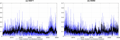
Notes. Realized Amihud (solid line) and daily Amihud (dashed line) for MSFT (for the ) and MMM (). Sample period: January 3, 2012, to January 10, 2024.
This paper contributes to the literature in two ways. First, it outlines a simple theoretical foundation for realized illiquidity. In developing it, we consider a setting where the instantaneous liquidity parameter, , follows a stochastic process in continuous time. We prove that the realized illiquidity provides a measurement of the integrated illiquidity, which is defined as the reciprocal of over periods of unit length (e.g., a day, a week, or a month). This allows us to establish how precisely the realized illiquidity measures the integrated illiquidity vis-à-vis the classic Amihud, which is a special case of the realized Amihud when only one observation per period (i.e., a daily return) is available. Because of its nonparametric nature, realized illiquidity provides a simple inverse measure of market resiliency—that is, the elasticity of asset prices with respect to trading volume, which in turn depends on the degree of disagreement among traders’ beliefs. We conclude the theoretical analysis by showing how the proposed framework can be extended to study spot illiquidity estimation and information jumps. Numerical analyses illustrate these theoretical features and show that, in controlled settings, the realized Amihud tracks the latent integrated illiquidity more closely than the classic daily Amihud, for both liquid and illiquid assets, even under market microstructure frictions.
Our second contribution is to empirically study realized illiquidity. To this end, we analyze the time-series and cross-sectional properties of a sample of U.S. stocks over the period from 2012 to 2024 using a comprehensive set of econometric specifications. Descriptive statistics comparing the realized Amihud with the classic Amihud indicate that average realized illiquidity rises monotonically as capitalization declines, whereas the classic Amihud fails to capture this expected pattern. Moreover, the distribution of the daily classic Amihud exhibits higher variance and greater leptokurtosis than that of the realized Amihud. At the individual-stock level, the realized Amihud is also markedly less noisy than the daily Amihud, particularly for large-cap stocks. Another simple yet meaningful analysis is whether realized illiquidity behaves similarly to established liquidity measures. We find that the realized Amihud aligns closely with the lambda factor of Kyle (1985) and other transaction-cost measures, whereas the classic daily Amihud exhibits substantially lower correlations.
We next examine the time-series properties of realized illiquidity. Our analysis sheds light on three main features. First, illiquidity exhibits pronounced clustering, with prolonged periods of high or low illiquidity reflecting persistent liquidity conditions over time. Second, this clustering is heterogeneous across horizons, with persistence at daily, weekly, and monthly frequencies. Using a multiplicative error model (MEM) (Engle and Gallo 2006), we show that such multiscale dependence renders illiquidity predictable over different time horizons. Third, realized illiquidity displays a leverage effect; liquidity deteriorates more following negative returns than it improves after positive returns of comparable magnitude, consistent with flight-to-liquidity dynamics and capital constraint mechanisms. Taken together, these properties are reminiscent of well-documented features of return volatility, namely persistence, predictability across multiple time scales,3 and asymmetric responses to negative versus positive shocks.
We conclude our empirical investigation by examining whether realized illiquidity predicts short-term stock returns. We find that the expected component of illiquidity positively predicts returns, whereas the unexpected component negatively predicts returns, with a substantially stronger effect. This pattern supports the notion that illiquidity shocks have persistent effects that raise expected future illiquidity and, in turn, depress stock prices. Importantly, these findings are significantly weaker when using the noisier, classic Amihud measure at both the market and individual stock levels.
Our paper contributes to the literature on market microstructure and market liquidity, which spans more than half a century (see, e.g., Silber 1975). The widespread use of the Amihud (2002) measure is due partly to its loose connection to the Kyle (1985) model, which provides a theoretical framework for how order flow impacts asset prices through the factor. However, measuring the order flow price impact requires access to comprehensive data on orders submitted by traders. Such data are often unavailable for many markets or data sets. In this context, the classic daily Amihud (2002) measure proves extremely useful for approximating the order flow impact on security prices because (a) it is an observable and nonparametric quantity and (b) it is based on daily price and volume data, which are far more accessible than tick-by-tick order and transaction data.4 However, using daily returns may introduce noise and imprecision because large intraday price movements in opposite directions can offset each other, obscuring the true sensitivity of prices to trading volume. Our realized Amihud measure retains advantage (a) but not (b) because achieving greater precision requires intraday returns to compute realized power variation. By incorporating intraday returns, the measure captures not only the daily net price movement but also cumulative intraday volatility—effectively quantifying the incremental sensitivity of prices to trading volume throughout the day. Although this refinement necessitates the use of intraday returns, it does not rely on tick-by-tick or order-book data. Instead, it can be constructed from preprocessed intraday data at one- or five-minute intervals, which are readily available through many commercial data vendors such as Bloomberg, FactSet, or Refinitiv. This offers a major practical benefit; the realized measure enhances informational content without the complexity and processing burden of tick-level data.
Barardehi et al. (2019) revisited the Amihud measure by developing a trade-time liquidity measure, which our theoretical framework is well suited to encompass. We calculate their measure and demonstrate that it correlates consistently with other illiquidity measures, including our own. Ranaldo and Santucci de Magistris (2022) adopted the realized Amihud to empirically investigate the price impact in the global FX market. We extend prior research in two key ways. First, we provide a general theoretical framework for realized illiquidity, with the Amihud ILLIQ measure arising as a specific case. Second, we study realized stock liquidity and document previously unexplored time-series features, such as heterogeneous clustering, leverage effects, and short-term return predictability. Our methodological approach is similar to that of Bandi et al. (2017, 2020, 2024), who investigated other aspects of illiquidity, such as zero returns and excess durations. In this work, we exploit a simple mechanism for generating trading volume and volatility, allowing us to derive the asymptotic properties of the realized Amihud as an estimator of integrated illiquidity.
2. A Simple Theory of Illiquidity Measurement
We develop a stylized reduced-form model of market volatility, trading volume, and liquidity, forming the basis of a nonparametric theory of illiquidity measurement inspired by Amihud (2002). Let us consider an asset traded on a financial market consisting of a finite number of active participants. Within each trading period of unit length (e.g., an hour, day, or week), the market evolves through a sequence of I intraperiod equilibria indexed by . The evolution of the equilibrium price is motivated by the arrival of new information to the market that changes the reservation prices of the traders. During intraperiod i, the quantity exchanged by the j-th trader is given by
The term is a positive parameter, and it captures the market depth. The larger the , the larger quantities of the asset can be exchanged for a given difference . For each trading interval , where , we define the liquidity parameter as the liquidity realized at the beginning of the interval, that is, , where is a càdlàg (or càglàd) stochastic process in continuous time. This choice is consistent with the standard practice of using information available at the start of a period to model trading dynamics within that period. The equilibrium function in (1) is analogous to the one outlined in Tauchen and Pitts (1983), which provides a stylized representation of the supply-demand mechanism on the market.5 The reservation price of each trader might reflect some of the following aspects: individual preferences, liquidity issues, asymmetries in information sets, and different expectations about the fundamental values of the asset. In general, the reservation price can deviate from the market price because of idiosyncratic reasons, inducing the j-th trader to trade. The quantity exchanged for a unit change of is given by the slope . In other words, measures the ability of the market to allow large quantities to be exchanged at the intersection between demand and supply, thus recalling the concept of market depth and resilience that reduces the price impact of trading. By market clearing, that is , we have that the average of the variations in the reservation prices clears the market, that is, . As new information arrives, traders adjust their reservation prices, , resulting in a change in the market price (), which is given by the average of the increments of the reservation prices. The trading volume in the i-th subinterval is given by
Using Equation (1), this can be written as
We assume that the reservation price of each trader evolves in continuous time according to the following process
In a reduced-form model of trading like the current one, the liquidity coefficient can evolve for several reasons that are not explicitly modeled, such as tightening of funding constraints, higher risk aversion of the market makers, or inventory rebalancing decisions. In particular, we assume that the liquidity process is driven by a continuous-time stochastic process fulfilling very mild regularity conditions, such as being strictly positive and càdlàg. For instance, may display deterministic diurnal effects, jumps, and long memory, lack an unconditional mean, or be nonstationary.
We define the realized Amihud as
Consider the illiquidity measure defined as , and assume an underlying filtered probability space satisfying the standard assumptions. Assume that is a strictly positive Itô’s semimartingale. Assume active traders, as representative of the two aggregated sides of the market, with being càglàd or càdlàg drift terms for . Because (i.e., ),
where indicates stable convergence, , and for , with and .
Proposition 1, whose proof is in Appendix A.1, shows that the realized Amihud is a measure of the inverse of the integrated liquidity ; namely, it is a measurement of the integrated illiquidity, which represents the price impact of trading volume cumulated over periods of unit length. The precision of the measurement increases with I and, the asymptotic distributions in (7) can be used to construct a confidence interval for and its log, respectively. Taking the ratio of volatility to volume isolates the price impact component of illiquidity from the volatility induced by information arrivals. Hence, by computing over disjoint periods of unit length (e.g., on daily horizons), one can obtain a time series of measurements of and use them to explore the evolution of illiquidity over time (see Section 3).
The quality of the realized Amihud as a measure of illiquidity is assessed through Monte Carlo simulations, where the daily horizon is taken as the reference unit interval and the liquidity process is modeled as an Ornstein-Uhlenbeck process on . As a representative illustration of the realized Amihud’s ability to accurately capture the latent illiquidity process, the left panel of Figure 2 displays the simulated time series of the daily “true” illiquidity signal (, shown in red) alongside its estimates (black dots), which are obtained by computing the realized Amihud at different intraday sampling frequencies (from 15 seconds to 1 hour). As the sampling frequency increases, the dispersion around the true illiquidity signal shrinks markedly and becomes negligible at both the 15-second and 1-minute intervals. The right panel of Figure 2 further shows that the distribution of the estimator increasingly approximates a Gaussian as the sampling frequency rises, consistent with the asymptotic result established in Proposition 1.
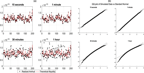
Notes. Panel (a) reports the true illiquidity limit (solid line) and the realized Amihud (dots) obtained by sampling returns at different frequencies of 15 seconds, 1 minute, 30 minutes, and 1 hour for a subset of 200 days. Panel (b) reports the QQ-plots of realized Amihud and illustrates the approximation to the Gaussian distribution of , as in (7).
The baseline Monte Carlo results are reported in Table 1.6 In this setup, the parameters governing the illiquidity process are calibrated via indirect inference using the time series of the realized Amihud for the DJ30 index, following the methodology of Corsi and Renò (2012) and Rossi and Santucci de Magistris (2018). Table 1 shows that the realized Amihud closely tracks the true integrated illiquidity process () across both low and high liquidity.7 The bias relative to the illiquidity signal remains below 0.5% in absolute terms, and the root mean squared error (RMSE) is small, even at moderate sampling frequencies (1–5 minutes). As implied by Proposition 1, the RMSE declines as the number of intraday intervals I increases (i.e., as decreases). Overall, the realized Amihud achieves significantly lower RMSE than the classic daily Amihud, which corresponds to the limiting case with a single observation per trading day (), where illiquidity reduces to .
|

Table 1. Illiquidity Measurement
| Low liquidity | High liquidity | |||||||
|---|---|---|---|---|---|---|---|---|
| Perc. Rel. Bias | Relative RMSE | Perc. Rel. Bias | Relative RMSE | |||||
| Sampling frequency | ||||||||
| 1h | 2.5064 | 2.5255 | 0.2367 | 0.8271 | 2.5047 | 2.9398 | 0.2364 | 0.8270 |
| 5min | 0.3320 | 0.3986 | 0.0645 | 0.7837 | 0.2087 | 0.5966 | 0.0648 | 0.7834 |
| 1min | 0.0117 | 0.1459 | 0.0291 | 0.7805 | 0.0338 | 0.3165 | 0.0292 | 0.7781 |
| 15sec | 0.0104 | 0.1431 | 0.0145 | 0.7798 | −0.0035 | 0.2641 | 0.0143 | 0.7771 |
Notes. This table reports the Monte Carlo percentage relative bias and RMSE (all relative to ) for two illiquidity estimators: the realized Amihud and the daily Amihud measure, that is, . The series is generated according to the log Ornstein-Uhlenbeck process with parameters (speed of mean reversion) and (volatility of innovations). Low liquidity is obtained setting , and high liquidity is obtained by setting . The smallest RMSE is in bold.
2.1. Extensions
It should be stressed that the asymptotic results (in the limit for ) behind Proposition 1 are derived by abstracting from several features that contribute to asset price formation. Although the baseline assumptions are stylized, they offer a tractable foundation for defining the concept of integrated illiquidity and developing a theory for its measurement. This theory can be refined to accommodate more sophisticated data-generating mechanisms, starting, for instance, from the equilibrium function in (1), which is linear in . This could be relaxed by replacing with a continuous monotonic function, for example, . In this case, Proposition 1 would still hold with replaced by . Similarly, the theoretical results in Section 2 are derived under a regular sampling grid, with . Notably, results in Proposition 1 remain valid even under irregular sampling schemes, that is, when trading within the interval [0,1] occurs in I subperiods , with , because . In this case, the length of the subintervals is a random variable. This allows for more advanced sampling techniques. For instance, in measuring illiquidity, the trade-time Amihud ratio by Barardehi et al. (2019) builds on the idea of an irregular sampling scheme that is driven by the amount of volume generated over a certain threshold.
Furthermore, Proposition 1 is derived under the assumption of two representative traders (), corresponding to the demand and supply sides of the market in each intraday period. Analogous results are obtained if , assuming homogeneity of traders, that is, . In particular, the following corollary to Proposition 1 highlights the main determinants of the realized Amihud as an illiquidity measure under homogeneity of traders when .
Consider the illiquidity measure defined as . Assume that is a strictly positive Itô’s semimartingale, with being càdlàg or càglàd drift terms and . Because (i.e., ),
It follows that in the limit for , the realized Amihud is inversely proportional to both integrated liquidity and the number of active traders in the market. In other words, the more active traders that are present on the market, the more the market is liquid (ceteris paribus the level of ). As an extension, the number of active traders could be assumed to follow a stochastic process for counts, for instance, a Poisson process, to allow for random entry and exit of traders. In the current context, the variation in illiquidity conditions depends only on variations in . In the special case with , we obtain the same limit of as in Proposition 1.
In the following paragraphs, we build on the theory of realized variance and introduce refinements to the theory of realized illiquidity measurement that ensure robustness to financial features such as stochastic volatility and market microstructure noise.8
2.1.1. Spot Illiquidity.
We extend the previous setting by allowing reservation prices (and hence, equilibrium prices) to follow the diffusive process in (3), with both the drift and the variance being time varying. In particular, the reservation prices are assumed to vary in continuous time according to the following law of motion,
These conditions restrict the local behavior of the volatility and liquidity processes while allowing for standard diffusion dynamics, including deterministic patterns, jumps, and non-stationarity, and are automatically satisfied when the mean, volatility, and liquidity processes have continuous trajectories. Allowing for trader-specific volatility captures several realistic features, including long memory in volatility arising from the superposition of traders operating at different frequencies. We propose the following estimator of instantaneous illiquidity, which we call spot Amihud, given by
Consider the illiquidity measure defined in (5), the equilibrium relation in (1), and the diffusive process for reservation prices in (3). Assume that and are strictly positive càdlàg processes for all . Assume active traders as representative of the two aggregated sides of the market. Because (i.e., ), with and , we obtain
Furthermore, , (with ), and ,
where the integral is approximated by the Riemann sum .
Proposition 2 demonstrates that, when both liquidity and volatility follow (potentially correlated) stochastic processes, spot (il)liquidity can be accurately measured using local estimators such as the spot Amivest (or spot Amihud). Although the realized Amihud is conceptually similar to the IDVOL measure of Lou and Shu (2017), the monthly averages of spot volatility estimates can be seen as a refined version of the monthly ILLIQ measure of Amihud (2002), as discussed in Amihud and Noh (2021, pp. 2103–2104). By relying on infill asymptotic arguments, our results eliminate the need to use expected values of the daily Amihud ratio, offering a direct theoretical link between IDVOL and ILLIQ.10
Panel (a) of Figure 3 displays the trajectory of the two-sided spot Amihud (computed using 1-minute intervals) over five consecutive trading days, from May 8–12, 2023. Panel (b) of Figure 3 reports the intraday average computed over one-minute intervals (black line, left-hand scale) and the difference between the intraday average on Mondays and the intraday average over all weekdays (red line, right-hand scale), for the full sample period. These parts of the figure suggest that stocks tend to be less liquid in the early part of the trading session than toward its end. Although a detailed analysis of these trading motives lies beyond the scope of this paper, a possible explanation is that the high information content accumulated overnight prompts large volume and price movements after the market opening, whereas less informative trading activity—often related to inventory rebalancing—shapes the later part of the trading session (see, e.g., Madhavan et al. 1997). Therefore, it is reasonable to maintain that the amount of information to be processed into prices is larger on Mondays because of the longer nontrading period over the weekend. Panel (b) of Figure 3 provides tentative evidence supporting this idea; the difference in intraday average illiquidity between Mondays and all weekdays is positive after the market opens.
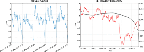
Notes. Panel (a) shows the 1-minute spot Amihud () for the market, computed as the market-capitalization-weighted average across 25 tickers from May 8–12, 2023, over the intraday period 9:45–15:45. Panel (b) reports the intraday average computed over 1-minute intervals (left-hand scale) and the difference between the intraday average on Mondays and the intraday average over all weekdays (right-hand scale) for the full sample period from January 3, 2012, to January 10, 2024.
2.2. Microstructure Frictions
In this section, we analyze the properties of the realized Amihud in a setting influenced by microstructural features such as transaction costs (bid-ask spreads, clearing fees), price discreteness, and staleness, all of which are interconnected and endogenous to the trading process. In microstructure models, following Kyle (1985) and Glosten and Milgrom (1985), informed traders play a key role in driving transaction prices; when the value of their information exceeds execution costs, they trade; otherwise, by refraining from trading, they may contribute to price staleness, as in Easley and O’Hara (1987).
To study the realized Amihud in this context, we adopt a reduced-form approach that consolidates all microstructural frictions into an additive noise term applied to the latent efficient price. This simplification obviates the need to explicitly model the price formation process between informed and uninformed traders, and it aligns with the semi-structural representations of mid-quote and transaction price dynamics proposed in Bandi et al. (2017, 2024), which offer a micro-foundation for price staleness. Although the simplified framework in Section 2 does not directly include these microstructural elements, their presence can substantially impact empirical analyses. Microstructure noise increases with sampling frequency and distorts volatility estimates. This challenge is well-documented in the realized variance literature, where moderate sampling frequencies (e.g., 5-minute intervals) are suggested to reduce noise contamination; see Liu et al. (2015).11
We explore the sampling frequency at which these microstructural frictions have a negligible effect on integrated illiquidity measurements. The microstructural features we consider—transaction costs, price discreteness—are intrinsic to the trading process and affect market microstructure. In these models, informed traders drive prices by acting when the value of their information exceeds transaction costs and refraining from trading otherwise, leading to price staleness. Specifically, in Table 12 in Section 1.4 of the Supplementary Document, we conduct Monte Carlo simulations incorporating bid-ask spreads and rounding mechanisms that induce price discreteness and zero returns (as described in Bandi et al. 2020). For instance, the bid-ask mechanism modifies observed log-prices as
Second, the realized Amihud measure remains robust in low-liquidity settings, providing accurate illiquidity measurements for less frequently traded securities. In summary, realized Amihud measures based on intermediate-frequency returns accurately capture illiquidity effects arising from price impacts, even in the presence of additional dimensions of illiquidity such as bid-ask spreads, staleness, and rounding. Further complexities, such as dependence between trading frictions across time and traders (e.g., spillover effects studied in Grossman and Miller 1988) or sequential trading behavior linked to crash episodes Christensen et al. (2022), require more advanced econometric techniques and granular data. Additionally, price rounding effects, as shown in Bandi et al. (2020), can generate a high frequency of zero returns, severely biasing the jump test statistics. Under such conditions, moderate sampling frequencies alleviate these biases even when the goal is to test for significant information jumps (see the right panel of Table 13 in the Supplementary Document), improving the accuracy of jump detection measures while retaining high power.
3. Empirical Analysis
We now turn to the empirical study of realized illiquidity, based on a sample of 25 stocks over the period from January 3, 2012, to January 10, 2024. The data are provided by Kibot, and the time series are constructed using one-minute intervals.12 The only exception is for bid and ask prices, which are recorded at tick-by-tick frequency.13 To assess whether our findings extend to less liquid assets, we also consider the low-capitalized stocks of the Standard and Poor’s 500 index.14
We examine the time-series and cross-sectional properties of daily (detrended) illiquidity as well as its relationship with stock returns. To represent the broader U.S. stock market, we calculated the return of a portfolio comprising these 25 stocks, weighted by their market capitalization; hereafter, we refer to this portfolio as the DJI. To streamline the presentation, we grouped individual stock returns into terciles based on market capitalization size.
Table 2 presents the sample statistics for the daily time series of the realized Amihud () and the classic Amihud () measures, which are calculated for the rescaled market portfolio. The table highlights three key findings. First, the average realized illiquidity consistently increases from the first tercile to the low-capitalized asset portfolio, whereas the daily Amihud measure does not exhibit this pattern. Second, the variance of the daily Amihud measure is significantly higher, reflecting its greater noise. Third, the classic Amihud measure exhibits a higher degree of leptokurtosis compared with its realized counterpart.
|
Table 2. Descriptive Statistics
| Mean | Variance | Skewness | Kurtosis | |||||
|---|---|---|---|---|---|---|---|---|
| DJI | 1.060 | 1.002 | 0.051 | 0.202 | 1.315 | 1.962 | 7.262 | 10.010 |
| 1st Tercile | 1.054 | 1.001 | 0.059 | 0.269 | 1.017 | 1.710 | 5.068 | 8.522 |
| 2nd Tercile | 1.065 | 1.006 | 0.055 | 0.174 | 2.087 | 1.751 | 14.118 | 8.307 |
| 3rd Tercile | 1.083 | 1.003 | 0.086 | 0.260 | 1.377 | 2.040 | 7.371 | 10.657 |
| Low-Cap | 1.103 | 1.012 | 0.116 | 0.224 | 2.405 | 1.656 | 15.561 | 7.864 |
Notes. The table reports the sample statistics for the daily time series of the realized Amihud () and the classic daily Amihud () for the DJI, that is, the average among 25 tickers weighted by their market capitalization, and the considered terciles. Both illiquidity measures are scaled by a factor of 1e11.
3.1. Stock Market Illiquidity
To introduce the analysis at the individual stock level, Figure 4 displays the average ratio of the time-series variance of the daily Amihud () to the realized Amihud () for each stock in our sample, with stocks ordered by market capitalization from highest to lowest along the horizontal axis. The figure shows that the variance of is typically three to six times higher. Moreover, the variance ratio tends to be larger for higher-capitalization stocks, whereas it equals 1.936 for the low-capitalized portfolio (green bar). This pattern suggests that provides a less noisy measure of realized illiquidity for more liquid stocks, likely because realized variance estimators are themselves noisier for illiquid stocks with fewer intraday trades. Importantly, because both measures are constructed by excluding the first and last 15 minutes of each trading session, the higher variance of the daily Amihud reflects the lower precision of this estimator, rather than being driven by overnight returns—as would be the case for close-to-close return-based measures. Although this exclusion may not fully eliminate the influence of overnight information, it implicitly assumes that such effects are absorbed largely within the first and last 15 minutes of trading.
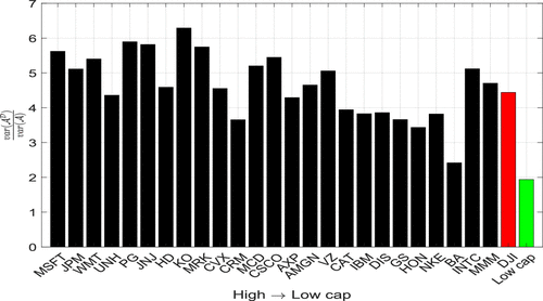
Note. Sample period: January 3, 2012, to January 10, 2024.
Another important question is whether the realized Amihud exhibits behavior similar to other well-established liquidity measures. Because it is designed to capture the price impact of trading volume, we expect a high correlation with Kyle’s lambda factor. To explore this, Table 3 presents the correlation matrix for daily illiquidity measures of the market portfolio, whereas correlations across sample terciles are provided in Section 3 in the Supplementary document. We compute pairwise correlations across three categories of liquidity measures. First, we consider volatility-over-volume measures, including the one-minute Realized Amihud (), the Realized Amihud computed using realized variance (), the Spot Amihud (), (Barardehi et al. 2019), and the classic daily Amihud (). 15 Second, we compute Kyle’s lambda (), the quoted bid-ask spread (BAS), and the effective cost (EC), which are common measures of transaction costs. Third, we consider well-established, low-frequency estimates of transaction costs, such as the High-Low spread estimator (Corwin and Schultz 2012) and the Close-High-Low estimator (Abdi and Ranaldo 2017), labeled CS and AR, respectively.
|
Table 3. Correlation Matrix for the Daily Illiquidity Measures for the DJI, That Is, the Average Among 25 Tickers Weighted by Their Market Capitalization
| BAS | EC | CS | AR | |||||||
|---|---|---|---|---|---|---|---|---|---|---|
| 1 | 0.986 | 0.993 | 0.773 | 0.361 | 0.666 | 0.599 | 0.465 | 0.441 | 0.310 | |
| 0.988 | 1 | 0.976 | 0.768 | 0.353 | 0.641 | 0.588 | 0.453 | 0.413 | 0.298 | |
| 0.992 | 0.977 | 1 | 0.775 | 0.366 | 0.689 | 0.618 | 0.484 | 0.473 | 0.333 | |
| 0.737 | 0.729 | 0.742 | 1 | 0.438 | 0.616 | 0.579 | 0.462 | 0.477 | 0.323 | |
| 0.309 | 0.296 | 0.318 | 0.375 | 1 | 0.319 | 0.289 | 0.224 | 0.342 | 0.235 | |
| 0.590 | 0.553 | 0.606 | 0.577 | 0.305 | 1 | 0.706 | 0.750 | 0.779 | 0.522 | |
| BAS | 0.481 | 0.463 | 0.489 | 0.512 | 0.291 | 0.527 | 1 | 0.932 | 0.688 | 0.478 |
| EC | 0.314 | 0.297 | 0.319 | 0.369 | 0.217 | 0.623 | 0.882 | 1 | 0.692 | 0.477 |
| CS | 0.297 | 0.259 | 0.323 | 0.410 | 0.365 | 0.662 | 0.497 | 0.512 | 1 | 0.547 |
| AR | 0.112 | 0.093 | 0.127 | 0.161 | 0.185 | 0.289 | 0.251 | 0.267 | 0.373 | 1 |
Notes. Pearson (Spearman) correlations are reported in the lower (upper) triangular portion of the table. is the 1-minute realized Amihud, is the realized Amihud computed with RV, is the spot Amihud, is the average per-dollar absolute returns of fixed-dollar volumes, and is the daily Amihud. is the Kyle lambda, BAS denotes the quoted bid-ask spread, EC the effective cost, CS the Corwin–Schultz spread estimator, and AR the Abdi–Ranaldo high–low spread estimator.
Three key findings emerge from the table. First, our measure exhibits a very high correlation with its alternative specifications ( and ) as well as a notably strong correlation with the estimate and the classic Amihud measure (). Second, the correlation between and Kyle’s lambda () is quite high, reinforcing the view that serves as a proxy for . Third, correlates strongly with other transaction cost proxies (BAS, EC, CS, and AR), further supporting its robustness as a liquidity measure. When comparing the correlations of and , it is important to highlight that the latter shows lower correlations with other liquidity proxies. Notably, the correlation between and is nearly half of that between and .16
A visual inspection of Figure 1 reveals that extended periods of low illiquidity are often followed by prolonged periods of high illiquidity. In the volatility literature, this phenomenon is well known as volatility clustering. Although prior research has clearly shown that liquidity follows a persistent pattern, we further investigate the empirical autocorrelation function (ACF) of both the classic and realized Amihud measures. As shown in Figure 5, the realized Amihud exhibits strong persistence, characterized by a slow decay in the ACF, which remains significantly high even after 50 lags. We refer to this as illiquidity clustering. In contrast, when we run the same autocorrelation analysis for the daily Amihud, we find much less persistence. This is typical behavior for persistent time series contaminated by additive noise, as highlighted by Hurvich and Ray (2003) and Hurvich et al. (2005) in the context of stochastic volatility estimation. Because the persistence of a phenomenon determines the duration of its shocks, this result highlights the importance of measuring liquidity with greater accuracy to capture the actual effects of illiquidity shocks.
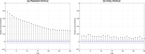
Note. Empirical autocorrelation function of the realized Amihud (left panel) and of the daily Amihud (right panel) for the DJI, that is, the average among 25 tickers weighted by the market capitalization.
An additional time-series property we want to highlight is whether illiquidity responds differently to negative stock price shocks (bad news) rather than to positive price shocks (good news). More specifically, we examine whether past return shocks asymmetrically affect future illiquidity. We call this mechanism leverage effect, which parallels a well-established characteristic of volatility, where negative return shocks increase volatility more than positive return shocks. Figure 6 displays the increase (in relative terms) in the realized illiquidity following a negative shock to returns for different time horizons, . Conversely, a positive shock to returns improves liquidity for many periods. Comparing the magnitude of these effects in absolute terms, we observe that past negative returns have a greater impact than positive returns of the same size.
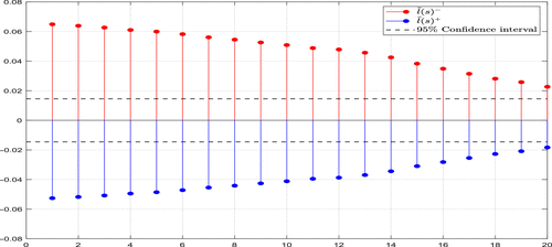
Notes. This figure reports the estimated propagation of the effect of a negative (upward red bars) and positive (downward blue bars) shock on returns on the realized Amihud. These quantities are computed as the empirical counterpart of , for . The estimators and are reported relative to the average illiquidity, that is, and . The black-dashed horizontal lines denote the 95% interval around 0.
Overall, three key stylized facts emerge from the time-series analysis of illiquidity. First, the realized Amihud measure exhibits less variability and a higher correlation with well-established liquidity measures compared with the classic Amihud. Second, illiquidity clusters over time, following a highly autocorrelated pattern. Third, negative returns have a stronger impact on illiquidity, leading to persistently higher autocorrelation in illiquidity. These findings justify the application of well-established volatility models for predicting illiquidity and motivate further investigation into the illiquidity-return dynamics, which we explore in the remainder of our paper.
3.2. Modeling Realized Illiquidity
We now examine a nonlinear dynamic specification to model the distributional characteristics of illiquidity and to assess the superiority of our measure over the classic Amihud measure in capturing these features. In particular, we consider a parametric model pertaining to the class of multiplicative error models (MEM), as introduced by Engle (2002) and Engle and Gallo (2006). Inspired by the heterogeneous autoregressive (HAR) model of Corsi (2009), we consider the MEM-AHAR model, as follows:
Table 4 presents the estimation results of the MEM-AHAR model applied to the realized Amihud (based on 1-minute returns) and to the classic daily Amihud. The first and sixth columns report the estimates for the market portfolio DJI, the second and seventh for the first tercile, the third and eighth for the second tercile, the fourth and ninth for the third tercile, and the remaining columns for the low-capitalization portfolio. Three key results emerge. First, today’s realized Amihud is significantly predicted by yesterday’s, last week’s, and last month’s illiquidity. This is supported by the estimated coefficients for , , and , which are all positive and highly significant at the 1% level. This finding confirms the presence of heterogeneous clustering of illiquidity across different time periods. Second, the original Amihud measure fails to capture this heterogeneity because the estimates are insignificant, whereas the monthly dependency is overstated with inflated coefficients, which is likely due to measurement errors. This suggests that the classic daily Amihud requires substantial smoothing to better separate the expected illiquidity signal from the noise in its ex post measurement. Similar evidence is found in the volatility literature when using the realized GARCH model of Hansen et al. (2012) compared with the classic GARCH model on squared returns. Specifically, the model assigns a smaller weight to the innovation term when there is a significant degree of measurement error. Additionally, the estimate (the reciprocal of the variance of ) for the classic daily Amihud is approximately 10 times smaller than that for the realized Amihud. This implies that the variability of the innovation term is 10 times higher when using the daily Amihud compared with the realized Amihud. Third, both measures detect an asymmetric response to return shocks, as indicated by a significant and positive estimate. This heterogeneous persistence of illiquidity is a novel finding that may have important implications for explaining stock returns over the short run, which we explore in the final part of this paper.
|
Table 4. MEM-AHAR Estimated Coefficients with Robust Standard Errors (In Parentheses) for the DJI (the Average Among 25 Tickers Weighted by the Market Capitalization), the 1st (Ordered by Market Capitalization), the 2nd, the 3rd Tercile, and for the Portfolio of the Low Capitalized Assets, That Is, the Average Among the Last 8 Tickers of the Standard and Poor’s 500 Index Weighted by the Market Capitalization
| DJI | 1st tercile | 2nd tercile | 3rd tercile | Low-cap | DJI | 1st tercile | 2nd tercile | 3rd tercile | Low-cap | |
|---|---|---|---|---|---|---|---|---|---|---|
| (0.0142) | (0.0145) | (0.0148) | (0.0126) | (0.0137) | (0.0413) | (0.0438) | (0.0386) | (0.0349) | (0.0320) | |
| 0.0000 | 0.0000 | 0.0093 | 0.0000 | 0.0337 | ||||||
| (0.0226) | (0.0224) | (0.0236) | (0.0242) | (0.0255) | (0.0261) | (0.0253) | (0.0250) | (0.0249) | (0.0268) | |
| (0.0334) | (0.0334) | (0.0361) | (0.0318) | (0.0375) | (0.0526) | (0.0526) | (0.0506) | (0.0531) | (0.0528) | |
| (0.0269) | (0.0275) | (0.0289) | (0.0249) | (0.0294) | (0.0613) | (0.0627) | (0.0595) | (0.0598) | (0.0549) | |
| 0.0236 | ||||||||||
| (0.0045) | (0.0051) | (0.0045) | (0.0053) | (0.0058) | (0.0148) | (0.0169) | (0.0135) | (0.0156) | (0.0160) | |
| (0.3627) | (0.4441) | (0.3886) | (0.3233) | (0.5427) | (0.2007) | (0.1217) | (0.2314) | (0.1624) | (0.2119) | |
Notes. Superscripts a, b, and c denote the 1%, 5%, and 10% significance levels, respectively. Sample period: January 3, 2012, to January 10, 2024.
3.3. Illiquidity and Stock Returns
In the final part of this paper, we analyze the relationship between illiquidity and stock returns over the short run. Building on Amihud (2002), we test two hypotheses. First, when investors anticipate higher illiquidity, they require a higher expected return. Second, higher expected returns imply that stock prices should decline when illiquidity unexpectedly increases. These mechanisms lead to two testable predictions: a positive relationship between expected illiquidity and asset returns and a negative relationship between unexpected illiquidity and contemporaneous asset returns. Whereas Amihud (2002) focused primarily on yearly and monthly horizons in an asset-pricing setting, we instead studied the short-run dynamics (daily, weekly, and monthly) of illiquidity and returns.
To operationalize these hypotheses, we decompose daily illiquidity into its expected and unexpected components. Following Amihud (2002), we estimate a univariate AR(1) model for each illiquidity series,
Table 5 reports the estimates for the DJI market portfolio at daily (), weekly, and monthly horizons, using both the realized Amihud and the classic daily Amihud. The first two columns report daily results. For the realized Amihud, the coefficient on expected illiquidity, , is positive and statistically significant, whereas the coefficient on unexpected illiquidity, , is negative and highly significant. Moreover, the magnitude of is about three times larger than that of , indicating that unexpected illiquidity has a stronger contemporaneous impact on returns than anticipated illiquidity. In contrast, when using the classic daily Amihud, both coefficients are statistically insignificant at the daily horizon.
|
Table 5. Regression of Stock Market Excess Returns on Illiquidity Decomposed into Expected and Unexpected Components, as Estimated from an AR(1) Model, for the DJI Portfolio (the Average Among 25 Tickers Weighted by Market Capitalization)
| Daily | Weekly | Monthly | ||||
|---|---|---|---|---|---|---|
| DJI portfolio | ||||||
| Intercept | −0.1238 | −0.0193 | 0.0187 | 0.0133 | 0.0469 | |
| (0.1292) | (0.2260) | (0.1155) | (0.0589) | (0.1079) | (0.0773) | |
| Expected illiquidity () | 0.1545 | 0.0489 | 0.0112 | 0.0161 | −0.0168 | |
| (0.1332) | (0.2264) | (0.1198) | (0.0643) | (0.1116) | (0.0822) | |
| Unexpected illiquidity () | 0.0085 | |||||
| (0.0167) | (0.0295) | (0.0110) | (0.0098) | (0.0059) | (0.0032) | |
| Diagnostic | ||||||
| 0.0663 | 0.0326 | 0.0988 | 0.0329 | 0.1637 | 0.0625 | |
| adj. | 0.0650 | 0.0313 | 0.0976 | 0.0316 | 0.1626 | 0.0612 |
| F-stat (p value) | 0.0000 | 0.0000 | 0.0000 | 0.0000 | 0.0000 | 0.0000 |
Notes. Coefficients and Newey and West (1987) robust standard errors (in parentheses) are scaled by a factor of 100. Superscripts a, b, and c denote the 1%, 5%, and 10% levels of significance, respectively.
At lower frequencies (weekly and monthly; columns 3–6), both illiquidity measures yield a significantly negative coefficient on unexpected illiquidity, , whereas is never statistically different from zero. Notably, the estimates derived from the classic Amihud are substantially smaller in magnitude than those obtained with the realized Amihud, consistent with the presence of measurement error in the daily Amihud.
We further extend the analysis across all horizons . For the realized Amihud, the estimated increases smoothly and monotonically with the horizon K. For the classic Amihud, instead declines and becomes significantly negative only for . Overall, the evidence indicates that the two hypotheses—a positive relation between expected illiquidity and returns and a negative relation between unexpected illiquidity and contemporaneous returns—are more clearly supported when using the more accurate realized Amihud measure.17
Panels (a) and (b) of Figure 7 display the estimated coefficients for individual stocks, along with 90% confidence intervals, for . In panel (a), based on the realized Amihud, the coefficient is negative and significant for 19 out of 25 stocks. In contrast, when using the classic Amihud (panel (b)), is positive and rarely significant (only 6 out of 25 stocks at the 10% level). Repeating the analysis for the DJI and the low-capitalized portfolios yields similar results. These findings further corroborate the superior performance of the realized Amihud at the daily frequency, including at the individual-stock level.
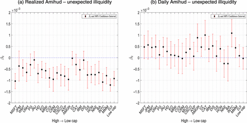
Notes. Panels (a) and (b) report the estimates of (black dots) in (17) for individual stocks at horizon using the realized Amihud and the daily Amihud, respectively. Red bars denote 90% confidence intervals.
4. Conclusion
Liquidity is essential to the efficient functioning of financial markets because it determines how trading volume affects asset prices. We develop a theory of realized illiquidity in which, similar to spot volatility, instantaneous liquidity is modeled as a stochastic process evolving over time in continuous time. Within this framework, we introduce a refined measure of realized illiquidity, which we term the realized Amihud.
Through theoretical and numerical analysis, we demonstrate that the realized Amihud offers a highly accurate estimate of the cumulative intraday price sensitivity to trading activity, enhancing the classic illiquidity measure proposed by Amihud (2002). Our findings show that the realized Amihud is significantly more precise and robust because it effectively accommodates features such as stochastic volatility, microstructure noise, information jumps, or possibly a (random) number of J traders that might diverge to infinity in some cases. This theoretical framework is scalable and may be extended to incorporate further microstructural complexities of market trading. Such developments could yield more refined measurement tools or provide theoretical foundations for advanced sampling schemes, such as the trade-time Amihud proposed by Barardehi et al. (2019). We believe these directions offer promising avenues for future research.
Empirical analysis of a sample of U.S. stocks reveals three main findings. First, the realized Amihud provides a less noisy and more stable measurement of market illiquidity. Second, time-series analysis uncovers persistent heterogeneity in illiquidity dynamics, including clustering and leverage effects. Third, the realized Amihud helps predict short-term stock returns, offering practical value for investors and researchers alike.
The authors are grateful to the department editor, Agostino Capponi, the anonymous associate editor, and three anonymous referees for their constructive comments and suggestions. The authors also thank Yakov Amihud, Tim Bollerslev, Nicola Borri, Massimiliano Caporin, Alessandro Casini, Leopoldo Catania, Kim Christensen, Dobrislav Dobrev, Deniz Erdemlioglu, Mark Hallin, Joel Hasbrouck, Fabrizio Lillo, Mark Podolskij, Anders Rahbek, Eduardo Rossi, Johannes Ruf, Francesco Sangiorgi, Pierluigi Vallarino, Bezirgen Veliyev, and Paolo Vitale for their relevant comments about the authors’ work. The authors are indebted to Orimar Sauri for his help in the derivation of the proof of Proposition 1. The authors also thank the participants at the Vieco Conference (Copenhagen University, 2022), the IAAE Conference (King’s College, 2022), the SoFiE Conference (Cambridge, 2022), the Rome-Waseda Time Series Symposium (Rome, 2022), the XXIV Quantitative Finance Workshop (Gaeta, 2023), the II Econometrics Workshop (Aarhus, 2023), the ICEEE Conference (Cagliari, 2023), the ESTA (Florianopolis, 2023), and the AFA (San Antonio, 2024), and the seminar participants at the IESEG School of Management, the Bank of Italy, the University of Pavia, Sapienza University of Rome, Luiss University, the University of Copenhagen, and EDHEC Business School.
Appendix A. Proofs
A.1. Proof of Proposition 1
The proof is structured as follows. We first establish consistency for RPV and the trading volume . We then prove a joint Central Limit Theorem (CLT) for and apply the delta method to obtain the asymptotic distributions of the realized Amihud ratio and its logarithm. Throughout, the observation interval is [0, 1], so .
A.1.1. Consistency.
We want to show , where . This is equivalent to showing that and that , with .
A.1.2. Consistency of RPV.
Let . We have to show that . Let us decompose , with , and write , where
By localization (lemma 4.4.9 in Jacod and Protter 2011), we may assume bounded; then, . Because the absolute value function is Lipschitz, it follows that , and hence, Because is independent of and ,
Hence,
A.1.3. Consistency of Volume.
Let . By construction,
For the martingale part,
Hence,
A.1.4. Central Limit Theorem.
We now prove the stable convergence in (7). Define
Let , with . Decompose , where
As in section 5.3.3 of Jacod and Protter (2011), we split with
Because, conditional on ,
Because is a positive Itô’s semimartingale, then the process satisfies assumption (K’) (Jacod and Protter 2011). Hence, the proof of (5.3.24) in Jacod and Protter (2011, pp. 153–154) applies, and . Now, set
Let , and then outside of B, f is continuously differentiable with
Therefore, equations (5.3.32) and (5.3.33) in Jacod and Protter (2011) apply with the terms and . Using this and lemmas 5.3.16 and 5.3.17 in Jacod and Protter (2011), we conclude that
Using once again the fact that the distribution of conditional on is Gaussian, it follows that , and . Therefore, , which shows that as required.
For Y, let denote the martingale obtained by removing drift terms (purely diffusive part). The Lipschitz property of f and standard semimartingale estimates (e.g., (5.2.11) in Jacod and Protter 2011) imply , where
We apply theorem 2.2.15 in Jacod and Protter (2011) to the triangular array . Condition (2.2.34) trivially holds (martingale differences). For condition (2.2.36), we have that
As for , define first the correlation of and as
By proposition 2 in Wellner and Smythe (2002),
Condition (2.2.37) (Lyapunov) holds because moments of functions of Gaussian variables are bounded and for any . Condition (2.2.40) follows from the Gaussianity of given . Thus , and therefore, .
By the delta method for stable convergence, for and ,
Hence
A.2. Proof of Corollary 1
The proof of Corollary 1 follows the same steps as the proof of Proposition 1. In this case,
Therefore,
A.3. Proof of Proposition 2
The proof of Proposition 2 is analogous, but now we focus on a spot volatility estimator as in Kristensen (2010).18 For , the spot variance estimator is
By theorem 3 in Kristensen (2010) and assumption K.1 on the kernel, we have
For the denominator of the spot Amihud,
Finally, by theorem 4 in Kristensen (2010), because , with , and ,
See theorem 9.2.1 in Jacod and Protter (2011) and Jacod and Rosenbaum (2013).
1 To date, the ILLIQ measure proposed by Amihud (2002) has been cited nearly 15,000 times, according to Google Scholar. Many of these papers were published in top-tier academic journals in finance.
2 Although the empirical analysis focuses on the realized illiquidity computed at daily frequency, our theory and metrics can be applied to shorter (intraday) or longer (e.g., weekly or monthly) horizons.
3 See, for example, the Heterogeneous Autoregressive model of realized volatility (HAR-RV) in Corsi (2009).
4 The accuracy of the Amihud (2002) measure has been well documented (Hasbrouck 2009). Fong et al. (2018) analyzed global and U.S. stocks using various liquidity proxies based on volatility over volume.
5 See also Clark (1973), Epps and Epps (1976), the survey in Karpoff (1987), and the empirical analysis in Andersen (1996).
6 The Supplementary Document (Section 1.1) provides detailed information on the simulation design and reports the robust outcomes of various Monte Carlo experiments.
7 The average liquidity levels () are calibrated to represent two distinct market environments, corresponding to a very liquid and a less liquid asset. The high-liquidity scenario is set with , matching the scale of the sample average of daily DJ30 liquidity, whereas the low-liquidity scenario is obtained using .
8 In Section 2 of the Supplementary Document, we also propose a version of the realized Amihud estimator robust to information jumps (i.e., large news common to traders). The estimator is based on the theory of multipower variation; see Barndorff-Nielsen and Shephard (2004) among others.
9 A vast and growing literature addresses the issue of consistently estimating spot volatility using high-frequency returns; see, among many others, the contributions of Foster and Nelson (1996), Mykland and Zhang (2009), Jacod and Rosenbaum (2013), Kanaya and Kristensen (2016), Bandi and Renò (2018), and Figueroa-lópez and Li (2020). In this section, we follow the notation and the set of assumptions outlined in Kristensen (2010).
10 Monte Carlo experiments (Section 1.2 in the Supplementary document) demonstrate that the estimator (based on (14)) of daily illiquidity performs comparably to, or better than, the realized Amihud () under stochastic volatility. This also holds at a monthly horizon (Section 1.3 in the Supplementary Document), where all realized Amihud measures are highly precise. Averaging daily Amihud () over a month further reduces variability but yields an estimator that is several times less efficient than the realized monthly measure.
11 Other approaches, such as the two-scales estimator Zhang et al. (2005), realized kernels Barndorff-Nielsen et al. (2008), and pre-averaging techniques Podolskij and Vetter (2009), have been proposed to address this issue (see also the survey in Aït-Sahalia and Jacod 2014).
12 Following standard practice, we exclude the first and last 15 minutes of the trading session to avoid distortions from opening and closing effects. As a robustness check, we also consider the full trading day; results (available upon request) remain fully consistent.
13 The tickers of the 25 stocks are AMGN, AXP, BA, CAT, CRM, CSCO, CVX, DIS, GS, HD, HON, IBM, INTC, JNJ, JPM, KO, MCD, MMM, MRK, MSFT, NKE, PG, UNH, VZ, and WMT.
14 The eight stocks are selected as those with the lowest average market capitalization over the sample period: BAX, CLX, CPB, IVX, MAS, TAP, TXT, and WBA.
15 We consider the proposed by Barardehi et al. (2019), which represents the average per-dollar absolute returns of fixed-dollar volumes.
16 Similar results hold when computing the same correlations separately for each tercile of stocks, including the low-cap portfolio; results are available upon request.
17 Full regression results for all horizons are reported in Section 4 of the Supplementary Document. We obtain similar results when conducting the same analysis on the low-capitalized portfolio (cf. Table 14). Although not statistically significant at , remains negative when using the realized Amihud, whereas it turns positive with the daily Amihud. At the weekly horizon, is significant only for the realized Amihud; at the monthly frequency, both estimators yield significantly negative coefficients.
18 See also Foster and Nelson (1996), Fan and Wang (2008), Mykland and Zhang (2008, 2009), Zu and Boswijk (2014), Kanaya and Kristensen (2016), Bandi and Renò (2018), and Figueroa-lópez and li (2020).
References
- (2017) A simple estimation of bid-ask spreads from daily close, high, and low prices. Rev. Financial Stud. 30(12):4437–4480.Crossref, Google Scholar
- (2014)
High-frequency financial econometrics . High-Frequency Financial Econometrics (Princeton University Press, Princeton, NJ).Google Scholar - (2002) Illiquidity and stock returns: Cross-section and time-series effects. J. Financial Markets 5(1):31–56.Crossref, Google Scholar
- (2021) Illiquidity and stock returns II: Cross-section and time-series effects. Rev. Financial Stud. 34(4):2101–2123.Crossref, Google Scholar
- (1996) Return volatility and trading volume: An information flow interpretation of stochastic volatility. J. Finance 51(1):169–204.Crossref, Google Scholar
- (2018) Nonparametric stochastic volatility. Econom. Theory 34(6):1207–1255.Crossref, Google Scholar
- (2017) Excess idle time. Econometrica 85(6):1793–1846. Crossref, Google Scholar
- (2024) Systematic staleness. J. Econometrics 238(1):1–38.Crossref, Google Scholar
- (2020) Zeros. Management Sci. 66(8):3466–3479.Link, Google Scholar
- (2019) Trade-time measures of liquidity. Rev. Financial Stud. 32(1):126–179.Crossref, Google Scholar
- (2003) Realized power variation and stochastic volatility models. Bernoulli 9(2):243–265.Crossref, Google Scholar
- (2004) Power and bipower variation with stochastic volatility and jumps. J. Financial Econom. 2(1):1–37.Crossref, Google Scholar
- (2008) Designing realized kernels to measure the ex post variation of equity prices in the presence of noise. Econometrica 76(6):1481–1536.Crossref, Google Scholar
- (2006)
A central limit theorem for realised power and bipower variations of continuous semimartingales . Kabanov Y, Liptser R, Stoyanov J, eds. From Stochastic Calculus to Mathematical Finance: The Shiryaev Festschrift (Springer, Berlin, Heidelberg), 33–68.Crossref, Google Scholar - (2022) The drift burst hypothesis. J. Econom. 227(2):461–497.Crossref, Google Scholar
- (1973) A subordinated stochastic process model with finite variance for speculative prices. Econometrica 41(1):135–155.Crossref, Google Scholar
- (2009) A simple approximate long-memory model of realized volatility. J. Financial Econom. 7(2):174–196.Crossref, Google Scholar
- (2012) Discrete-time volatility forecasting with persistent leverage effect and the link with continuous-time volatility modeling. J. Bus. Econom. Statist. 30(3):368–380.Crossref, Google Scholar
- (2012) A simple way to estimate bid-ask spreads from daily high and low prices. J. Finance 67(2):719–760.Crossref, Google Scholar
- (1987) Price, trade size, and information in securities markets. J. Financial Econom. 19(1):69–90.Crossref, Google Scholar
- (2002) New frontiers for ARCH models. J. Appl. Econom. 17(5):425–446.Crossref, Google Scholar
- (2006) A multiple indicators model for volatility using intra-daily data. J. Econom. 131(1–2):3–27.Crossref, Google Scholar
- (1976) The stochastic dependence of security price changes and transaction volumes: Implications for the mixture-of-distributions hypothesis. Econometrica 44(2):305–321. Crossref, Google Scholar
- (2008) Spot volatility estimation for high-frequency data. Statist. Interface 1(2):279–288.Crossref, Google Scholar
- (2020) Optimal kernel estimation of spot volatility of stochastic differential equations. Stochastic Processes Appl. 130(8):4693–4720.Crossref, Google Scholar
- (2018) Are volatility over volume liquidity proxies useful for global or US research? Kelley School of Business Research Paper No. 17-49.Google Scholar
- (1996) Continuous record asymptotics for rolling sample variance estimators. Econometrica 64(1):139–174.Crossref, Google Scholar
- (2013) Market Liquidity: Theory, Evidence, and Policy (Oxford University Press, Oxford, UK).Crossref, Google Scholar
- (1985) Bid, ask and transaction prices in a specialist market with heterogeneously informed traders. J. Financial Econom. 14(1):71–100.Crossref, Google Scholar
- (1993) On the relation between the expected value and the volatility of the nominal excess return on stocks. J. Finance 48(5):1779–1801.Crossref, Google Scholar
- (1988) Liquidity and market structure. J. Finance 43(3):617–633.Crossref, Google Scholar
- (2012) Realized GARCH: A joint model for returns and realized measures of volatility. J. Appl. Econom. 27(6):877–906.Crossref, Google Scholar
- (2009) Trading costs and returns for us equities: Estimating effective costs from daily data. J. Finance 64(3):1445–1477.Crossref, Google Scholar
- (2003) The local Whittle estimator of long-memory stochastic volatility. J. Financial Econom. 1(3):445–470.Crossref, Google Scholar
- (2005) Estimating long memory in volatility. Econometrica 73(4):1283–1328.Crossref, Google Scholar
- (2011) Discretization of Processes, Stochastic Modelling and Applied Probability (Springer Berlin Heidelberg).Google Scholar
- (2013) Quarticity and other functionals of volatility: Efficient estimation. Ann. Statist. 41(3):1462–1484.Crossref, Google Scholar
- (2016) Estimation of stochastic volatility models by nonparametric filtering. Econom. Theory 32(4):861–916.Crossref, Google Scholar
- (1987) The relation between price changes and trading volume: A survey. J. Financial Quant. Anal. 22(1):109–126.Crossref, Google Scholar
- (1936) The General Theory of Employment, Interest, and Money (Palgrave Macmillan, London, UK).Google Scholar
- (2010) Nonparametric filtering of the realized spot volatility: A kernel-based approach. Econom. Theory 26(1):60–93.Crossref, Google Scholar
- (1985) Continuous auctions and insider trading. Econometrica 53(6):1315–1335.Crossref, Google Scholar
- (2015) Does anything beat 5-minute RV? A comparison of realized measures across multiple asset classes. J. Econom. 187(1):293–311.Crossref, Google Scholar
- (2017) Price impact or trading volume: Why is the Amihud (2002) measure priced? Rev. Financial Stud. 30(12):4481–4520.Crossref, Google Scholar
- (1997) Why do security prices change? A transaction-level analysis of NYSE stocks. Rev. Financial Stud. 10(4):1035–1064.Crossref, Google Scholar
- (2008) Inference for volatility-type objects and implications for hedging. Statist. Interface 1(2):255–278.Crossref, Google Scholar
- (2009) Inference for continuous semimartingales observed at high frequency. Econometrica 77(5):1403–1445.Crossref, Google Scholar
- (1987) A simple, positive semi-definite, heteroskedasticity and autocorrelation consistent covariance matrix. Econometrica 55(3):703–708.Crossref, Google Scholar
- (2009) Bipower-type estimation in a noisy diffusion setting. Stochastic Processes Appl. 119(9):2803–2831.Crossref, Google Scholar
- (2022) Liquidity in the global currency market. J. Financial Econom. 146(3):859–883.Crossref, Google Scholar
- (2018) Indirect inference with time series observed with error. J. Appl. Econom. 33(6):874–897.Crossref, Google Scholar
- (1975) Thinness in capital markets: The case of the Tel Aviv stock exchange. J. Financial Quant. Anal. 10(1):129–142.Crossref, Google Scholar
- (1983) The price variability-volume relationship on speculative markets. Econometrica 51(2):485–505.Crossref, Google Scholar
- (2002) Computing the covariance of two Brownian area integrals. Statistica Neerlandica 56(1):101–109.Crossref, Google Scholar
- (2005) A tale of two time scales: Determining integrated volatility with noisy high-frequency data. J. Amer. Statist. Assoc. 100(472):1394–1411.Crossref, Google Scholar
- (2014) Estimating spot volatility with high-frequency financial data. J. Econom. 181(2):117–135.Crossref, Google Scholar

