Large-System Insensitivity of Zero-Waiting Load Balancing Algorithms
Abstract
This paper studies the sensitivity (or insensitivity) of a class of load balancing algorithms that achieve asymptotic zero-waiting in the sub-Halfin-Whitt regime, named LB-zero. Most existing results on zero-waiting load balancing algorithms assume the service time distribution is exponential. This paper establishes the large-system insensitivity of LB-zero for jobs whose service time follows a Coxian distribution with a finite number of phases. This result justifies that LB-zero achieves asymptotic zero-waiting for a large class of service time distributions as the Coxian family is dense in the class of positive-valued distributions. To prove this result, this paper develops a new technique, called “iterative state-space peeling” (ISSP). ISSP first identifies an iterative relation between the upper and lower bounds on the queue states and then proves that the system lives near the fixed point of the iterative bounds with a high probability. Based on ISSP, the steady-state distribution of the queue length is further analyzed by applying Stein’s method in the neighborhood of the fixed point. ISSP, like state-space collapse in heavy-traffic analysis, is a general approach that may be used to study other complex stochastic systems.
1. Introduction
Zero-wait load balancing refers to a load balancing algorithm in which a job is routed to an idle server and is processed immediately on its arrival. The zero-waiting property has become increasingly important as the amount of modern machine learning (ML) and artificial intelligence (AI) applications running on large-scale data centers explodes. Although increasing the number of servers and the processing speed of each server is a critical step to meet the increasing demand, the design of load balancing algorithms that can efficiently use available resources to minimize or even eliminate the waiting time of incoming jobs is equally important, especially when a minor increase of latency (e.g., 100 milliseconds) can lead to a significant drop in a cloud-computing provider’s revenue (7% drop in sales according to a recent Akamai report; Akamai 2017).
Significant progress has been made over the past few years on achieving asymptotic zero-waiting (as the system size approaches infinity) in a large-scale data center with distributed queues, including the classic supermarket model (Stolyar 2015; Mukherjee et al. 2016; Banerjee and Mukherjee 2018; Eschenfeldt and Gamarnik 2018; Liu and Ying 2018, 2020, 2021; Gupta and Walton 2019; Braverman 2020; Liu et al. 2021), models with data locality (Weng et al. 2020, Rutten and Mukherjee 2022), and models where each job consists of parallel tasks (Weng and Wang 2020, Hong and Wang 2021, Wang et al. 2021).
However, almost all these results assume exponential service time distributions. Although each of these results provided important insights into achieving zero-waiting in a practical system, theoretically, it is not clear whether these principles hold for general service times. This is a very important question to answer because it is well known that service time distributions in real-world systems are not exponential. Understanding a queueing system’s performance with general service times remains one of the most important and intensively studied problems in stochastic networks (Schelling 1978, Whittle 1985, Zachary 2007). A concept that excited many theorists in the area is “insensitivity” (Burman 1981). A queueing system is called insensitive if the steady-state distribution of queue lengths is invariant to the service time distribution. Therefore, any conclusion drawn from exponential service time distributions can be applied to general service time distributions. A result that is insensitive is robust and is expected to be widely applicable in practical systems. Unfortunately, insensitivity results are rare and often hold only under some special queueing disciplines such as processor sharing (PS) (Burman 1981, Bonald et al. 2004, Jonckheere and Prabhu 2018, Kielanski and Van Houdt 2021). One of the reasons is that insensitivity, although appealing, is a very strong notion of “robustness.” It requires the steady-state distribution under a general service time distribution to be exactly the same as that under the exponential distribution. Some recent studies started to relax it to weaker notions such as insensitivity in the heavy-traffic regime (Wang et al. 2018) or the large-system regime (Bramson et al. 2012, Stolyar 2015), that is, insensitivity in the limiting regimes. In the light of these recent developments, this paper addresses the following important question:
Are the zero-waiting algorithms insensitive and if so, for which notion of insensitivity?
1.1. Main Contributions
This paper provides some positive answers to the previous question. First, it is well known that most zero-waiting algorithms, such as join-the-shortest-queue (JSQ) (Winston 1977) and join-the-idle-queue (JIQ) (Lu et al. 2011), are not insensitive (according to its original definition). However, we prove that in the sub-Halfin-Whitt regime, LB-zero identified in Liu and Ying (2020) in fact achieves asymptotic zero-waiting for jobs whose service time follows a Coxian distribution with a finite number of phases. (Informally speaking, LB-zero refers to a class of load balancing algorithms that assigns an incoming job to an idle server with a high probability and achieves asymptotic zero-waiting. The formal definition is in Section 3.) This result establishes the large-system insensitivity of LB-zero for Coxian service time distributions with a finite number of phases in the sub-Halfin-Whitt regime. Because the Coxian family is dense in the class of positive-valued distributions, our result justifies load balancing algorithms in the LB-zero family will be able to minimize unnecessary waiting in large-scale data centers for a large class of job size or service time distributions.
To prove this result, this paper develops a new technique, called “iterative state-space peeling” (ISSP). ISSP first identifies an iterative relation between upper and lower bounds on the queue states. Then by iteratively “peeling off” the low-probability states, it proves that the system “lives” near the fixed point of the iterative bounds with a high probability. Based on ISSP, the steady-state distribution of the system can be further analyzed by using Stein’s method in a small neighborhood of the fixed point, where in the large-system regime, the queue lengths under LB-zero behave similarly as an system because almost all incoming jobs are immediately assigned to an idle server, so we can expect some insensitivity. ISSP, like the state-space collapse in the heavy-traffic analysis, is a general technique that may be used to study other complex stochastic systems, for example, large-system insensitivity of load balancing algorithms for other models such as Mukherjee et al. (2018), Weng and Wang (2020), Weng et al. (2020), and Wang et al. (2021).
We remark that this paper does not establish the large-system insensitivity for an arbitrary service time distribution, for which we need to show that our results continue to hold for a large but finite N when the number of phases of the Coxian distribution goes to infinity. This requires an interchange limit argument or a continuity argument and is an interesting open problem. It is also worth mentioning that a Coxian representation of a probability distribution is nonunique. The choice of the Coxian representation is out of the scope of this paper.
1.2. Related Work
Steady-state analysis of distributed queueing systems has been an active research topic since the seminal work on power-of-two-choices (Mitzenmacher 1996, Vvedenskaya et al. 1996). The most popular approach to study a large-scale distributed queueing system is the mean-field approach where the system is approximated using a deterministic dynamical system (a set of ordinary differential equations), called a mean-field model. In the large-system limit (as the number of servers approaches infinity), the steady state of the stochastic system can often be shown to converge to the equilibrium point of the mean-field model using the interchange of limits (Vvedenskaya et al. 1996, Xie et al. 2015, Ying et al. 2015) or Stein’s method (Ying 2016, Gast 2017).
Although most studies on this topic assume exponential service time distributions for tractability, the approach has been used to study nonexponential service time distributions theoretically or numerically (Mitzenmacher 1996, Gupta et al. 2007, Bramson et al. 2012, Stolyar 2015, Aghajani et al. 2017, Hellemans and Van Houdt 2018, Van Houdt 2019, Vasantam et al. 2019, Kielanski and Van Houdt 2021). Gupta et al. (2007) studied JSQ load balancing with processing sharing service discipline and established its insensitivity property. When the service time distribution has a decreasing hazard rate (DHR), the system often exhibits a monotonicity property such that the system starting from the empty state is dominated by the system starting from any other state. Leveraging this monotonicity, Bramson et al. (2012) proved the convergence of power-of-d-choices (pod), and Stolyar (2015) proved the convergence of JIQ to the corresponding mean-field limit, respectively. Recently, Van Houdt (2019) studied load balancing policies under the hyper-exponential service time distribution in the light traffic regime (or in a critical traffic regime). By transforming the hyper-exponential distribution to a Coxian distribution with DHR, the monotonicity property holds in a partial order and the global stability of the mean-field model was established. Kielanski and Van Houdt (2021) studied Pod with PS servers for a hyper-exponential distribution of order 2 in the light traffic regime. They also established the global stability result in a spirit similar to Van Houdt (2019). Kielanski and Van Houdt (2021) considered Pod where d is a constant independent of the number of servers so the system has a nonvanishing delay in the large-system limit. For the Pod algorithm to be in the LB-zero family, d is a function of N and the algorithm achieves asymptotic zero waiting in the heavy-traffic regime without the DHR assumption.
Without DHR, the results are very limited. Bramson et al. (2012) proved the convergence of join the least loaded of d queues (LL(d)) for general service time distributions and that of Pod when the load of the system is small (less than 1/4). Foss and Stolyar (2017) proved the asymptotic optimality of JIQ under general service time distributions when the normalized load is less than 0.5 (asymptotic optimality means as the steady-state probability of an arriving customer being routed to a nonidle server vanishes). Because JIQ is an LB-zero policy, our result confirms the conjecture made in Foss and Stolyar (2017) that JIQ is asymptotically optimal for any load less than one and not just less than 0.5. Another significant result is Bonald et al. (2004), which identifies a set of policies that are insensitive in many-server load-balancing systems and are optimal in the class of insensitive load balancing algorithms. The asymptotic blocking probability of this class of insensitive algorithms in a finite buffer system was later studied in Jonckheere and Prabhu (2018). Many LB-zero such as JSQ and Pod algorithms are sensitive, so the results in Bonald et al. (2004) and Jonckheere and Prabhu (2018) do not apply. The waiting probability in our paper includes both blocking (we consider server systems with finite buffer size and jobs are possible to be blocked) and being queued in the buffer, so our result implies asymptotic zero blocking of LB-zero in the sub-Halfin-Whitt regime.
Liu et al. (2021) is the work most related to this paper, which considers the Coxian-2 distribution and shows that LB-zero achieves asymptotic zero-waiting in the sub-Halfin-Whitt regime. Inspired by Liu et al. (2021), this paper develops the ISSP technique for general Coxian distributions with a finite number of phases and establishes its large-system insensitivity. We remark that Liu et al. (2021) used a key property of Coxian-2 service time distribution that a job in the first phase (phase 1) either departs or enters the last phase (phase 2) immediately, which does not hold under a general Coxian distribution which may have many phases because a job starting in phase 1 requires going through the intermediate phases before entering the last phase. The intermediate phases complicate the dependence among states and make the analysis much more challenging. Technically speaking, it requires a dedicated partition and aggregation of the states for a general Coxian distribution such that the upper/lower bounds on the steady-state distribution can be established in an iterative way. Such an iterative analysis is not necessary in Coxian-2.
In terms of the proof, each step in ISSP uses the tail bound in Bertsimas et al. (2001) to “peel off” a low probability subspace. The tail bound is based on the Lyapunov drift analysis and is a critical step to prove state-space collapse in the traditional heavy traffic regime with a fixed number of servers (Eryilmaz and Srikant 2012, Maguluri and Srikant 2016, Wang et al. 2018). The key difference is that Eryilmaz and Srikant (2012) use the tail bound only once, whereas ISSP repeatedly uses the tail bound guided by an iterative relation between the upper and lower bounds.
2. Model and State Representation
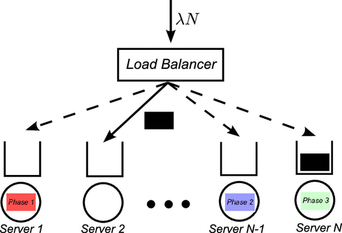
We consider a many-server system with N homogeneous servers, where job arrival follows a Poisson process with rate λN with , that is, the system is in the sub-Halfin-Whitt regime. We assume the service times follow the Coxian distribution with M phases as shown in Figure 1, where is the rate a job finishes phase m when in service and is the probability that a job enters phase i + 1 after completing phase i and We assume for the ease of exposition, but our results can be easily extended to the case that with any positive constant independent of N. As convention, we define if a > b and if a > b for the series

Note. μm is the service rate in phase m, and pm is the probability of entering phase m + 1 after finishing service in phase m.
Without loss of generality, we normalize the mean service time to be one, that is,
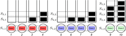
Taking a Coxian-3 distribution as an example (Figure 2), a job is colored in black if it waits in the buffer, and colored in light red, blue, and green when it is in phases 1, 2, and 3, respectively. Jobs are served with the first in first out (FIFO) discipline, and we assume each server has a buffer of size so can hold at most b jobs (b − 1 in the buffer and one in service). The assumption of finite buffer is imposed due to a technical reason and will be explained later in the paper (specifically, it is required when proving state-space collapse argument in Lemma F.2). Relaxing the finite-buffer assumption is not trivial, but we conjecture that our results hold without this assumption.
Note. Jobs colored in black, light red, blue, and green represent jobs in the buffer in phases 1, 2, and 3, respectively.
To represent the system, define () to be the fraction of servers that have j jobs at time t and are serving a job in phase m. Because an idle server does not have a phase, we define to be the fraction of servers that are idle at time t and for convenience. Let be a matrix such that the (j, m)th entry of the matrix is We further define and Therefore, is the fraction of servers that have at least i jobs and are serving a job in phase m at time t and is the fraction of servers with at least i jobs at time t. Stack to be a matrix S(t) such that the (j, m)th entry of the matrix is Because there is a one-to-one mapping between Q(t) and S(t), we focus on S(t) throughout the paper. We consider load balancing policies which dispatch jobs to servers based on S(t) and under which the finite-state continuous-time Markov chain (CTMC) is irreducible, and so it has a unique stationary distribution. This includes well-known load balancing policies such as JSQ (Winston 1977, Eschenfeldt and Gamarnik 2018, Braverman 2020), JIQ (Lu et al. 2011, Stolyar 2015), I1F (Gupta and Walton 2019), and Pod (Mitzenmacher 1996, Vvedenskaya et al. 1996).
Let be a random variable that has the distribution of at steady state. Correspondingly, define and In other words, is the fraction of servers that have at least i jobs and are serving a job in phase m, and Si is the fraction of servers with at least i jobs, both at steady state. Consider a system with 10 servers and Coxian-3 service time distribution. A realization of state representation is shown in Figure 3. Define to be a matrix such that the (i, m)th entry is and to be a realization of S. Define to be a set of s as follows:
that is, is the set of all possible s in a system with N servers. Note is a set defined for the scaled states.
3. Main Results
We introduce LB-zero load balancing policies and main results in this section. Let be the probability that an incoming job is routed to a busy server given that the system is in state that is,
We now consider the set of zero-waiting load balancing policies, named as LB-zero,
This class of policies is similar to the one considered in Liu and Ying (2020). Several well-known policies satisfy this condition, as summarized in Table 1.
|

Table 1. Examples of LB-Zero Policies: Join-the-Shortest-Queue, Join-the-Idle-Queue, Idle-One-First, and Power-of-d-Choices with a Carefully Chosen d
| Load balancing policy | Description | Condition |
|---|---|---|
| Join-the-Shortest-Queue | Route an incoming job to the least loaded server | for |
| Join-the-Idle-Queue | Route an incoming job to an idle server if available and otherwise, to a server chosen uniformly at random. | for |
| Idle-One-First | Route an incoming job to an idle server if available; to a server with one job if available; and otherwise, to a randomly selected server. | for |
| Power-of-d-Choices with | Sample d servers uniformly at random and route the job to the least loaded server among the d servers. | For sufficiently large N, for |
To prove the large-system insensitivity of LB-zero, we first show that is “close” to which is the normalized load from phase m of the jobs and is also the equilibrium point of the mean-field system assuming zero-waiting (details can be found in Sections 4 and 5). We call the zero-waiting equilibrium. Theorem 1 shows that at the steady state, concentrates around the zero-waiting equilibrium for large N under any LB-zero policy. The proof of this theorem can be found in Section 6.
There exist positive constants θm with independent of N. For any LB-zero policy in the following result holds for a large N:
Theorem 1 shows that differs from by at most with a probability at least which implies the convergence to the steady-state to the zero-waiting equilibrium as in probability and mean-square senses, that is, ( as ). To be best of our knowledge, this is the first result to establish such a steady-state convergence for a load balancing system under Coxian-M service time distributions in the sub-Halfin-Whitt regime. Because the high probability bound holds for a large but finite N, it also provides a rate of convergence. The specific requirement on N and values of constants θm can be found in Section 6 and Appendix A, respectively.
From Theorem 1, we have the following corollary on the distance between the steady-state and its mean-field equilibrium
When N is sufficiently large, LB-zero policies in Π achieve
From Theorem 1 and Corollary 1, it is not clear whether the probability of waiting approaches zero under an LB-zero policy because the average number of waiting jobs (per server) is not clear yet. This will be studied in the next theorem and its key step is to establish the upper bound on the average queue length in Lemma 6. Let denote the event that an incoming job is routed to a busy server in the system, and denote the probability of this event at steady state. We have the following result on the waiting probability. The proof of Theorem 2 can be found in Section 7.
For any LB-zero policy in the following result holds for a large
Theorem 2 shows that the waiting probability is for a large but finite N, which implies the asymptotic zero waiting, that is, as in the sub-Halfin-Whitt regime. This asymptotic result implies LB-zero is large-system insensitive to Coxian-M distributions with a finite number of phases. The specific requirement on N can be found in Section 7.
Next, we will establish these two main results. We first introduce the system dynamic of LB-zero in Section 4 and present ISSP in Section 5, which is used to prove that the system lives near a limiting regime in Theorem 1 in Section 6 and to prove the large system insensitivity in Theorem 2 in Section 7. A roadmap can be found in Figure 4, which demonstrates the relationship of the key lemmas and theorems. The condition in LB-zero is used when we analyze the dynamics of or including Lemma 1 in ISSP (the lower bound on ) and “zero-waiting” in Theorem 2 and its associated intermediate Lemma F.2.
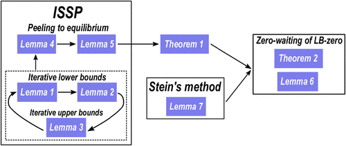
Notes. Lemmas 1–3 establish the iterative upper and lower bounds, which are used to establish Lemma 4 and 5 and Theorem 1. Together with Stein’s method in Lemma 7, zero-waiting is established in Lemma 6 and Theorem 2.
4. System Dynamics
Define to be a b × M-dimensional matrix with the (i, m)th entry being and all other entries being zero. Furthermore, define to be the probability that an incoming job is routed to a server with at least i jobs and the job in service is in phase m given the system state s, that is,
Given state s (or the corresponding q) of the CTMC, each of the following three events triggers a state transition, which is illustrated individually in Figure 5.
Event 1: A job arrives and is routed to a server that has i − 1 jobs and the job in service is in phase m as in the left figure in Figure 5. When this occurs, increases by and decreases by (note m = 1 if i = 1 since we define the fraction of idle servers to be ). Therefore, the CTMC has the following transition:
where the transition of s can be verified according to the definition so only increasing by This event occurs with ratewhere is the probability that an incoming job is routed to a server that has i − 1 jobs and the job in service is in phase m.Event 2: A server with i jobs finishes serving a job in phase m, and the job departs from the system without entering into the next phase as in the middle figure in Figure 5. When this event occurs, decreases by and increases by so the CTMC has the following transition:
where the transition of s can be verified based on the definition so decreases by for any and increases by for any This event occurs with ratewhere is the rate at which a job in phase m finishes the service and is the probability that a job finishes phase m and departs from the system immediately.Event 3: A server with i jobs finishes serving a job in phase m, and the job enters the next phase m + 1 as shown in the right figure in Figure 5. When this event occurs, a server in state (i, m) transits to state so decreases by and increases by Therefore, the CTMC has the following transition:
where the transition of s holds because decreases by for any and increases by for any This event occurs with ratewhere is the rate at which a job in phase m finishes the service and pm is the probability that a job enters phase m + 1 after finishing phase m.
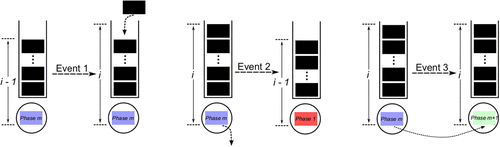
Note. (1) A job arrives to a server with i − 1 jobs and the job in service in phase m; (2) a server with i jobs finishes a job in phase m, and the job departs from the system; and (3) a server with i jobs finishes a job in phase m, and the job enters into the next phase.
Define G to be the generator of CTMC Given function we have
To understand the dynamics better, we write down the mean-field model (MFM) according to the generator:
This mean-field model is nonlinear in s because is a nonlinear function in s () and its equilibrium point is difficult to calculate in general. However, suppose zero-waiting occurs, that is, and the fraction of jobs dropped is negligible, then we can obtain the following equilibrium:
We call zero-waiting equilibrium because it is a conjectured equilibrium by assuming zero-waiting. Note zero-waiting equilibrium corresponds to the mean-field model in (5)–(6) with only and for any . In this following analysis, we will not solve Mean-Field Model (5)–(6) to check whether its equilibrium is close to . Instead, we will directly prove concentrates around and zero waiting occurs at the steady state with a high probability.
5. ISSP
In this section, we illustrate the key idea of ISSP, which will be applied to prove Theorem 1. Intuitively, the original stochastic system and the steady-state would be close to the MFM and the zero-waiting equilibrium respectively. However, because of the “nonmonotonicity” of the system (the “monotonicity” means a partial order of two systems starting from two initial conditions will be maintained over time), it is extremely challenging to justify this argument. To tackle the challenge, we develop a new technique, called ISSP, which first identifies an iterative relation between upper and lower bounds on the original stochastic queue states and then proves that the system lives in a regime concentrated around the “fixed point” of the iterative bounds with a high probability. We outline the general steps to apply ISSP. The key step is to identify the lower and upper bound functions according to the drift (or dynamics) of the mean-field model such that if the system is in region 1, then it leaves region 1 and moves toward region 2 with a rate (or drift) of x. The drift will provide a high probability upper or lower bound on the steady-state distribution. In particular, if the mean-field system leaves a region with a certain rate, then the probability that the steady-state system is in this region is low.
In particular, we focus on the fraction of busy servers with the job in service in phase m because we hypothesize (in other words, the fraction of servers with any waiting jobs is negligible in a large system).
Let n be the nth step of ISSP. Let denote a high probability lower bound on and be a high probability upper bound on established at the nth step of ISSP, that is,
5.1. ISSP: Hand-Waving Explanation
In this section, we present a hand-waving explanation of our ISSP, which is based on the following iterative relation between the upper and lower bounds on the queue states, denoted by and
We next provide a hand-waiving argument to show these equations iteratively provide upper and lower bounds. The exact definitions of and and their relations can be found in (15)–(17). The formal proofs that establish these are indeed high-probability upper and lower bounds can be found in Section 6. The right-hand sides of (7)–(9) can be regarded as the iterative update to refine the upper and lower bounds. Considering (7), given holds with a high probability, we can establish holds with a high-probability and the formula of is given in the right-hand side in (7). Considering (8), given holds with a high-probability, we can establish holds with a high probability, where the formula of is given in the right-hand side in (8). Considering (9), given and holds with a high probability, we can establish with a high probability, where the formula of is given in the right-hand side in (9).
From (7)–(9), we can obtain a recursive equation for
Therefore, as and
To provide the intuition behind (7)–(9), we consider the mean-field model under JSQ as an example and focus on in (5)–(6) by ignoring that is,
We next carefully analyze (11)–(12) to establish (7)–(9). To derive the lower and upper bounds on the equilibrium point of a dynamical system x(t) (or ), we use the following straightforward ideas. We need to emphasize that these are intuitive ideas and informal arguments to guide us to formalize ISSP in Section 6.
If
(13)then x(t) eventually becomes greater than or equal to L, that is, because otherwise x(t) continues to increase.If
(14)then x(t) eventually becomes smaller than or equal to U, that is, because otherwise, x(t) continues to decrease.
In the following, we will explain (7)–(9) based on the previous ideas. The explanation is not a rigorous proof. The detailed proof will be presented later in Section 6. We will ignore the iteration index n occasionally when confusion does not arise.
The intuition to obtain (7): We start with the dynamic of in (11), which is
The intuition to obtain (8): Consider the dynamic of in (12):
Given we have
Note so we have which means that the ratio of the lower bounds is the same as that of the corresponding equilibrium points.
The intuition to obtain (9): We focus on the dynamic of that
Given and we have
By invoking we eventually have
5.2. ISSP: Illustrative Example
To demonstrate ISSP, we consider JSQ with Erlang-3 distribution and no buffer, that is, Erlang-3 with
The mean-field model under JSQ with Erlang-3 and
With the Erlang-3 service time distribution, we have
Therefore, the MFM in this case is
ISSP for JSQ with Erlang-3 and The values of the key parameters in iterative equations in this case are and The corresponding iterative equations are
The iterative relation in terms of is
The iterative procedure has been visualized in Figure 6. In each iteration n, we first establish (shown in light red) based on from the last iteration, and then obtain (shown in light blue) based on and (shown in light green) based on Given the new lower bounds on we first refine (shown in light purple) and finally establish given all the new lower bounds and upper bound which in turn will improve in the next iteration.
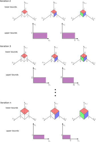
Note. The lower bounds of keep increasing and the upper bounds of and keep decreasing until reaching the equilibriums: the initial values (at iteration 1) are the lower bounds increase as ; the upper bound U2 of decreases as the upper bound U3 of decreases as
In the following sections, we formalize the ISSP, which is then combined with Stein’s method to prove Theorems 1 and 2.
6. Proof of Theorem 1 Based on ISSP
In this section, we formalize ISSP to prove Theorem 1. We first present the formal definitions of the iterative Equations (7)–(9) in the following:
These iterative lower and upper bounds are proved to hold with high probability in the following lemmas, that is,
The probability are diminishing quantities for a large N. The specific values of and positive constants can be found in Appendix A. We only state the lemmas and their proofs can be found in Appendix C.
A lower bound on given The following lemma is the rigorous statement of (7).
Given
A lower bound on given : The following lemma is the rigorous statement of (8).
Consider Given
An upper bound on given and The following lemma is the rigorous statement of (9).
Consider Given
6.1. Convergence of
Based on Lemmas 1–3, we will show is an increasing sequence and approaches
Given and we have
6.2. Proving Theorem 1
Because is an increasing sequence before reaching its equilibrium, we can apply Lemma 4 a sufficient number of times so that is close to which is formalized in the following lemma. We can keep applying Lemma 4 because both the lower bound and the probability only depend on the previous iteration and .
To prove this lemma, we apply Lemma 4 n times iteratively with such that We obtain
Recalling and noting we have
The result in Lemma 5 established that
Combining with Lemma 2, we next prove that holds with a high probability. Applying Lemma 2 iteratively for we have
Therefore, we have proved the lower bound in the theorem.
Define the event We have according to the union bound. We now establish the upper bound in Theorem 1 as follows:
The proof is completed because
7. Proof of Theorem 2
Theorem 1 shows that is “close” to with a high probability. However, it is not clear whether the average total queue length or the waiting probability is small under an LB-zero policy because Theorem 2 alone does not quantify the expected total queue length and the waiting probability. To establish Theorem 2, we first prove an important lemma on the upper bound of the average total queue, which is used to establish the waiting probability in Theorem 2 by the Markov inequality. The proof of this lemma can be found in Sections 7.1–7.3.
Define , and Under a load balancing policy in LB-zero, the following bound holds:
Lemma 6 establishes an upper bound on the average total queue length. Recall Theorem 1 indicates the service rate under an LB-zero policy in Π is close to arrival rate λN at steady state because Therefore, it is reasonable to couple the distributed load balancing system with a simple centralized server system with a similar arrival rate and service rate. This coupling will be done via Stein’s method (Braverman et al. 2016, Ying 2016). Stein’s method allows us to understand the key performance metrics (e.g., average queue length) of a complicated load balancing system from the performance of a simple fluid system (to be introduced in the next section). Formally, we study the generator difference between the distributed load balancing system and a simple centralized system within a small state space identified by ISSP. This idea of coupling a simple (and almost trivial) fluid model, without ISSP, has been also used in Liu and Ying (2020, 2021) and Liu et al. (2021). We will introduce it next so the paper is self-contained. Generator coupling in Section 7.1 and state space peeling in Section 7.2 are used to prove Lemma 6.
7.1. Generator Coupling with a Single Server System
Denote We consider a single server queue with arrival rate λ and service rate The fluid model with respect to the queue length x is
Let function g(x) be the solution of the following Stein’s equation or Poisson equation (Ying 2016) for the fluid system above and distance function h(x) such that
To analyze the total queue length at steady state under an LB-zero policy in we choose a truncated distance function:
To couple the one-dimensional fluid system in (18) with the b × M-dimensional stochastic system, we define
Note f(s) is bounded for and we imply the generator of stochastic system G defined in (2)–(4) on function f and have the basic adjoint relationship for the stationary distribution S such that
Combining (19) and (21), we connect the performance metric with the generator difference between the simple single-server system and G as follows:
In the following lemma, we provide an upper bound on (22) that includes two terms: the first term is from the gradient bounds and the second term is from ISSP. The proof of this lemma can be found in Appendix D.
Define the regions and denote the normalized service rate then we have
To establish Lemma 6 and Theorem 2 based on the previous lemma, we need to provide the upper bounds on (24), which are related to the difference between the normalized arrival rate and the normalized service rate, which will be bounded based on the ISSP result that shows the normalized service rate at the steady state is close to the zero-waiting equilibrium value.
7.2. State Space Peeling on
We analyze J1 in (24) by splitting it into two cases and show it is in Section 7.3:
We define two regions and :
Case 1: In Lemma E.1, we show any satisfies
It implies for any For any we have
It implies for any
Case 2: In Lemma F.1, we show that
using an ISSP approach on S1 and
Therefore, (25) are nonpositive under and under , respectively, as shown in Section 7.3.
7.3. Proving Lemma 6
Recall (25) Based on the two regions and , we split (25) into these two regions as follows:
The first item in (27) is negative because Lemma E.1 shows for any and for any Therefore, we have
By combining (23) and (28), we can now establish Lemma 6 in the following:
7.4. Proving Theorem 2
Once we have Lemma 6, we can prove Theorem 2 with the property of LB-zero and the Markov inequality. For an LB-zero policy in the waiting probability satisfies
Finally, we remark that we choose to prove Lemma F.2, which is the technical reason we assumed b is finite. We, however, believe our results hold even for
8. Simulations
In this section, we confirm our theoretical results of ISSP in Theorem 1 and the large system insensitivity in Theorem 2 with simulations. We considered two policies, JSQ and JIQ, and We conjecture that our results hold even for because it holds for any To confirm this, we used in our experiments (the additional experiments with and can be found in Appendix G). We set the buffer size b = 10, and in our simulations, no blocking events were observed.
8.1. Large System Insensitivity Under JSQ and JIQ
We first studied the average total queue length (per server) and the waiting probability under a Coxian-4 service time distribution with the parameters and We plotted and versus the number of servers N. The results are obtained with 10 trials, and each trial has 107 steps. From Figure 7, the waiting probability tends to zero when N increases as we expected and JIQ almost has the identical performance as JSQ. We then investigated and versus Coxian-M with various number of phases M and fixed In particular, we consider Coxian-M with and where and (identical service times). We plotted and versus M. From Figure 8, we can observe that the average queue length and the waiting probability remain roughly the same under different Ms, which confirms the insensitivity.
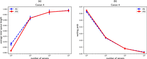
Notes. (a) Average queue length per server. (b) Waiting probability.
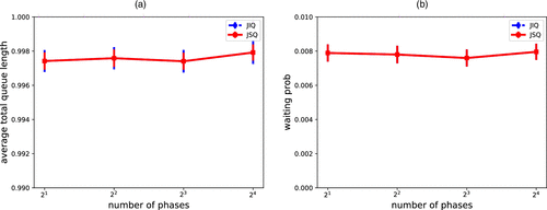
Notes. (a) Average queue length per server. (b) Waiting probability.
8.2. ISSP Under JSQ and JIQ
In this section, we investigated ISSP by studying the trajectory of under JSQ and JIQ. We considered n = 10,000 and a Coxian-4 service time distribution with and We plotted of JSQ and JIQ in Figure 9. The results are obtained with 10 trials, and each trial has 106 steps. We observed that under both policies concentrates around dash lines which confirms the high probability bounds in one. The system was initialized with the zero-waiting equilibrium instead of the empty state in our simulations.
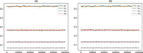
Notes. (a) Trajectories under JSQ. (b) Trajectories under JIQ.
We also provide additional experiments in Appendix G. These additional results justify the finite buffer assumption and demonstrate the performance of LB-zero under different traffic intensities and the service time distributions with different variations.
9. Conclusions and Discussions
In this paper, we studied a distributed queueing system under Coxian service time distributions in the sub-Halfin-Whitt regime. We established that a set of load balancing policies, named LB-zero, achieves asymptotic zero-waiting, that is, insensitive in the large-system regime. To tackle the nonmonotonicity under general service time distributions, we developed a technique, called iterative state-space peeling (ISSP), which iteratively removes the low-probability states, and results in a small state-space that can be analyzed using a simple mean-field model. This ISSP approach may be used for other problems as well. One possible application is to study load-balancing in many server systems with heterogeneous servers or jobs belonging to multiple priority classes. For heterogeneous servers, we can use ISSP to identify the “typical” load of each type of the servers; and for jobs with different priorities, we can use ISSP to identify the “typical” distribution of job types in the system. In the reduced state space based on the typical load of the typical distribution at the steady state, the steady-state performance of the many server system may become tractable like in this paper.
A conference version of this paper was published as a two-page extended abstract in ACM Sigmetrics/IFIP performance 2022 in Liu et al. (2022). The submission is the full version, including all details and technical proofs. This work was done when K. Gong was at the University of Michigan, Ann Arbor.
Appendix A. Definition of the Constants and Tail Probability
We introduce the positive constants that are used throughout the paper:
We will prove the constants and CM are positive in the next lemma, and in Lemmas A.1 and A.2. We also introduce the iterative tail probabilities:
The following two lemmas show that the constants () and CM are positive, and
The constants and CM are positive.
Note holds by the definition. Therefore, it is easy to verify and CM are positive.
Next, we prove is positive as follows:
Recall the definition of We have
Appendix B. Proof of Corollary 1
According to Theorem 1, we have for a large N,
It implies
Moreover, let the event and its complementary we have
Appendix C. Proof of the Lemmas for Theorem 1
We first prove Lemmas 1–4 used in ISSP.
C.1. Tail Bound from Wang et al. (2018)
We introduce lemma 10 from Wang et al. (2018), which is an extension of the tail bound in Bertsimas et al. (2001) and is the key to establishing ISSP. Lemma C.1 allows us to apply the Lyapunov drift analysis to iteratively reduce the state space.
Let be a continuous-time Markov chain over a finite state space and is irreducible, so it has a unique stationary distribution that is, Consider a Lyapunov function and define the drift of V at a state as
Assume there exists a set with B > 0, such that the following conditions hold
(i) when and
(ii) when and
Then
According to Lemma C.1, the critical step in establishing the tail bound is to construct proper Lyapunov functions. In the following sections, we construct a sequence of Lyapunov functions and apply Lemma C.1 to prove Lemmas 1–4. In the following proofs, we ignore the iteration number n for a clean notation.
C.2. Proof of Lemma 1: Lower Bound on Given
Given
To prove Lemma 1 using Lemma C.1, we consider the following Lyapunov function:
When and we have
(a) holds because when for a LB-zero policy in Π and
(b) holds because
(c) holds because and
(d) holds because
Moreover, we have for any
Define The maximum drift in (C.2) is μ1, and we define We now apply Lemma C.1 with Because and we have
(a) holds by substituting and
(b) holds based on Lemma C.1; and
(c) holds because and the assumption of the lemma on
C.3. Proof of Lemma 2: Lower Bound on Given for
Consider Given
To prove Lemma 2, consider Lyapunov function
Define
Given we have
Therefore, the drift of V(s) when and is
(a) holds according to the definition of
(b) holds because and
(c) holds because
Moreover, we have for any
Define The maximum drift in (C.4) is μm, and we define Combining and we have
Applying Lemma C.1 with we have
(a) holds by substituting and
(b) holds based on Lemma C.1; and
(c) holds because
C.4. Proof of Lemma 3: Upper Bound on Given and
Consider Given
Consider Lyapunov function
Given and we have
(a) holds because and
(b) holds because for any and implied by and
(c) holds by the definition of
Moreover, we have for any ,
We now apply Lemma C.1 with Define Maximum drift in (C.5) is , and we define Because and we have
(a) holds by substituting and
(b) holds based on Lemma C.1; and
(c) holds because and union bounds on
Now we prove which serves the upper bound on , and we represent Um with Recall the definition of from the previous section that
Therefore, we have
C.5. Proof of Lemma 4: Convergence of
In this section, we show that approaches as n increases (with a gap no larger than ). The key intuition to prove the results is based on the mean-field equilibrium and verify if can also increase and approach its equilibrium.
Given and we have
Starting from we can apply Lemma A.1 to obtain lower bounds for and then apply Lemma A.2 to obtain upper bounds for all including Then from we obtain new lower bound This iterative process implies that and are both a function of as shown below. Recall that in Lemma 3, we obtained
By recursively substituting we can write UM as a function of as follows:
Let us consider
Next we study the probability of given From Lemma 2, we have
By expanding the previous inequality from ϵM until it implies that
Therefore, we have
Last, we prove the “monontocity” improvement of by studying
Appendix D. Proof of Lemma 7
According to the definition of and f(s) in (20), we have
Substituting the generator equation to (22), we have
According to (19), it is easy to verify
Also, when
By using mean-value theorem in the region and Taylor theorem in the region we have
In (D.8) and (D.9), we have that
Given we have
From the definition of g function in (19), we have
Hence, for any we have
For we have
From the definition of g function in (19), we have
For we have
Based on gradient bounds in Lemmas D.1 and D.2 and we have
Appendix E. Lemma E.1 and Proof
For any
We consider the following linear programming problem:
Recall The minimum value is achieved when the maximum mass is allocated to such that Therefore, we have
(a) holds because and takes
(b) holds because and
(c) holds because given carefully chosen and
Appendix F. Lemma F.1 and Proof
For a large N, we have
The proof of Lemma F.1 again relies on iterative state space peeling, which is based on Theorem 1 and Lemma F.2.
(
Based on Theorem 1 and Lemma F.2, we define sets and such that
According to the union bound and Theorem 1 and Lemma F.2, we have
We note that is a subset of This is because for any s that satisfies
Note that
We therefore have
Next, we prove Lemma F.2.
F.1. Proof of Lemma F.2
Recall and Let and
Consider Lyapunov function
When the following two inequalities hold:
We have two observations based on (F.4) and (F.5):
(F.4) implies that under any LB-zero policy in Π;
(F.5) implies that because and we have
(F.6)where a finite buffer size is required such that the lower bound is meaningful.
We next study the Lyapunov drift when and by considering two cases:
Suppose In this case, and
(F.7)where○ (a) holds because under any policy in
○ (b) holds because of (F.6); and
○ (c) holds because
Suppose In this case, and
(F.8)(F.9)where○ (a) holds because
○ (b) holds because and
○ (c) holds because given k and and
○ (d) holds because
Next, we further show based on the upper bounds (F.7) and (F.8).
Consider the upper bound in (F.7). We have
where holds becauseConsider the upper bound in (F.8). We have
where the last inequality holds because
We now apply Lemma A.2. Define and Combining and we have
Choosing we have
(a) holds by substituting and
(b) holds based on Lemma A.2;
(c) holds because
(d) holds by union bounds on and
(e) holds because and
Appendix G. Additional Experiments
In this section, we provide additional experiments justifying our theoretical results. Specifically, we verify if the assumption of the finite buffer is proper for LB-zero, test LB-zero under the different traffic intensity levels, and the service times distributions with varying coefficients of variation.
G.1. Finite Buffer Assumption
We run the experiments for JIQ with and under Coxian 4 (this setup intuitively is most likely to introduce large queue lengths). The results are plotted in Figure G.1, where we observe even are extremely small and is always zero. This implies a small buffer size is sufficient for “zero-waiting” load balancing.
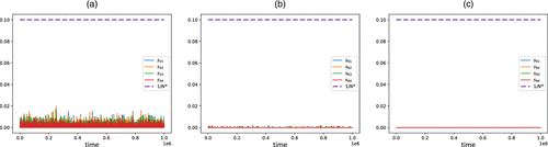
Notes. (a) The trajectory of . (b) The trajectory of . (c) The trajectory of .
G.2. Varying Traffic Intensity
We run the experiments for LB-zero under the different traffic intensity besides We choose and that satisfy the heavy-traffic assumptions. The buffer size is still set to be 10. The results are shown in Figures G.2 and G.3, respectively, where we observe the similar asymptotic zero waiting results as in the case of in Figure 7. Moreover, it is shown that the waiting probabilities become smaller as α decreases.
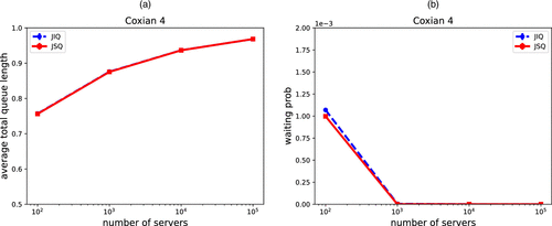
Notes. (a) Average queue length per server. (b) Waiting probability.
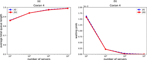
Notes. (a) Average queue length per server. (b) Waiting probability.
G.3. Varying Coefficients of Variation
We run the experiments for LB-zero under service time distributions with varying coefficients of variation (COV). In particular, we considered the hyper-exponential service with varying when in Figure G.4. The buffer size is set to a slightly larger value b = 50 to ensure almost no job is blocked. In fact, we did not observe any blocking events in the experiment. The results demonstrate that the waiting probability becomes larger as COV increases and that JSQ achieves a smaller average queue length per server than JIQ. Interestingly, we observe JSQ has a larger waiting probability than JIQ as COV increases. The intuition is that JSQ behaves like a single server queue system due to the effect of resource pooling, so when the variance is relatively large, a “large job” is more likely to block small jobs (head of line blocking), which results in a large waiting probability but with small waiting time.
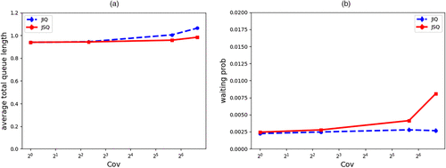
Notes. (a) Average queue length per server. (b) Waiting probability.
References
- (2017) The PDE method for the analysis of randomized load balancing networks. Proc. ACM Measurement Anal. Comput. Systems, vol. 1 (ACM, New York), 1–28.Google Scholar
Akamai (2017) The state of online retail performance report, Cambridge, MA.Google Scholar- (2018) Join-the-shortest queue diffusion limit in Halfin-Whitt regime: Tail asymptotics and scaling of extrema. Preprint, submitted September 28, https://arxiv.org/abs/1803.03306.Google Scholar
- (2001) Performance of multiclass markovian queueing networks via piecewise linear lyapunov functions. Ann. Appl. Probabilities 11(4):1384–1428.Google Scholar
- (2004) Insensitive load balancing. Performance Evaluation Rev. 32(1):367–377.Google Scholar
- (2012) Asymptotic independence of queues under randomized load balancing. Queueing Systems 71(3):247–292.Google Scholar
- (2020) Steady-state analysis of the join-the-shortest-queue model in the Halfin-Whitt regime. Math. Oper. Res. 45(3):1069–1103.Link, Google Scholar
- (2016) Stein’s method for steady-state diffusion approximations: An introduction through the Erlang-A and Erlang-C models. Stochastic Systems 6:301–366.Link, Google Scholar
- (1981) Insensitivity in queueing systems. Adv. Appl. Probabilities 13(4):846–859.Google Scholar
- (2012) Asymptotically tight steady-state queue length bounds implied by drift conditions. Queueing Systems 72(3–4):311–359.Google Scholar
- (2018) Join the shortest queue with many servers. The heavy-traffic asymptotics. Math. Oper. Res. 43(3):867–886.Link, Google Scholar
- (2017) Large-scale join-idle-queue system with general service times. J. Appl. Probabilities 54(4):995–1007.Google Scholar
- (2017) Expected values estimated via mean-field approximation are 1/n-accurate. Proc. ACM Measurement Anal. Comput. Systems, vol. 1 (ACM, New York), 1–26.Google Scholar
- (2019) Load balancing in the nondegenerate slowdown regime. Oper. Res. 67(1):281–294.Link, Google Scholar
- (2007) Analysis of join-the-shortest-queue routing for web server farms. Performance Evaluation 64(9–12):1062–1081.Google Scholar
- (2018) On the power-of-d-choices with least loaded server selection. Proc. ACM Measurement Anal. Comput. Systems, vol. 2 (ACM, New York), 1–22.Google Scholar
- (2021) Sharp waiting-time bounds for multiserver jobs. Preprint, submitted September 11, https://arxiv.org/abs/2109.05343.Google Scholar
- (2018) Asymptotics of insensitive load balancing and blocking phases. Queueing Systems 88:243–278.Google Scholar
- (2021) On the asymptotic insensitivity of the supermarket model in processor sharing systems. Proc. ACM Measurement Anal. Comput. Systems, vol. 5 (ACM, New York), 1–28.Google Scholar
- (2018) On achieving zero delay with power-of-d-choices load balancing. Proc. IEEE Internat. Conf. Computer Comm., vol. 6 (IEEE, Piscataway, NJ), 909–916.Google Scholar
- (2020) Steady-state analysis of load balancing algorithms in the sub-Halfin-Whitt regime. J. Appl. Probabilities 57(2):578–596.Google Scholar
- (2021) Universal scaling of distributed queues under load balancing in the super-Halfin-Whitt regime. IEEE/ACM Trans. Networks 30(1):190–201.Google Scholar
- (2021) Steady-state analysis of load balancing with Coxian-2 distributed service times. Naval Res. Logist. 69(1):57–75.Google Scholar
- (2022) Large-system insensitivity of zero-waiting load balancing algorithms. Proc. ACM SIGMETRICS/IFIP PERFORMANCE Joint Internat. Conf. Measurement and Modeling of Comput. Systems (ACM, New York), 101–102.Google Scholar
- (2011) Join-idle-queue: A novel load balancing algorithm for dynamically scalable web services. Performance Evaluation 68(11):1056–1071.Google Scholar
- (2016) Heavy traffic queue length behavior in a switch under the maxweight algorithm. Stochastic Systems 6(1):211–250.Link, Google Scholar
- (1996) The power of two choices in randomized load balancing. PhD thesis, University of California, Berkeley, CA.Google Scholar
- (2018) Asymptotically optimal load balancing topologies. Proc. ACM Measurement Anal. Comput. Systems (ACM, New York), 14:1–14:29.Google Scholar
- (2016) Universality of power-of-d load balancing in many-server systems. Preprint, submitted December 2, https://arxiv.org/abs/1612.00723.Google Scholar
- (2022) Load balancing under strict compatibility constraints. Math. Oper. Res. 48(1):227–256.Google Scholar
- (1978) Micromotives and Macrobehavior (Norton, New York).Google Scholar
- (2015) Pull-based load distribution in large-scale heterogeneous service systems. Queueing Systems 80(4):341–361.Google Scholar
- (2019) Global attraction of ODE-based mean field models with hyperexponential job sizes. Proc. ACM Measurement Anal. Comput. Systems, vol. 3 (ACM, New York), 1–23.Google Scholar
- (2019) Insensitivity of the mean field limit of loss systems under SQ(d) routeing. Adv. Appl. Probabilities 51(4):1027–1066.Google Scholar
- (1996) Queueing system with selection of the shortest of two queues: An asymptotic approach. Problemy Peredachi Informatsii 32(1):20–34.Google Scholar
- (2021) Zero queueing for multi-server jobs. Proc. ACM Measurement Anal. Comput. Systems, vol. 5 (ACM, New York), 1–25.Google Scholar
- (2018) Heavy-traffic delay insensitivity in connection-level models of data transfer with proportionally fair bandwidth sharing. Performance Evaluation Rev. 45(3):232–245.Google Scholar
- (2020) Achieving zero asymptotic queueing delay for parallel jobs. Proc. ACM Measurement Anal. Comput. Systems, vol. 4 (ACM, New York), 1–36.Google Scholar
- (2020) Optimal load balancing with locality constraints. Proc. ACM Measurement Anal. Comput. Systems, vol. 4 (ACM, New York), 1–37.Google Scholar
- (1985) Partial balance and insensitivity. J. Appl. Probabilities 22(1):168–176.Google Scholar
- (1977) Optimality of the shortest line discipline. J. Appl. Probab. 14(1):181–189.Google Scholar
- (2015) Power of d choices for large-scale bin packing: A loss model. Proc. Ann. ACM SIGMETRICS Conf. (ACM, New York), 321–334.Google Scholar
- (2016) On the approximation error of mean-field models. Proc. Ann. ACM SIGMETRICS Conf. (ACM, New York), 285–297.Google Scholar
- (2015) The power of slightly more than one sample in randomized load balancing. Proc. IEEE Internat. Conf. Computer Comm. (IEEE, Piscataway, NJ), 1131–1139.Google Scholar
- (2007) A note on insensitivity in stochastic networks. J. Appl. Probabilities 44(1):238–248.Google Scholar