


The Longest-Chain Protocol Under Random Delays
Abstract
In the field of distributed consensus and blockchains, the synchronous communication model assumes that all messages between honest parties are delayed by at most a known constant Δ. Recent literature establishes that the longest-chain blockchain protocol is secure under synchronous communication. However, these security guarantees degrade with Δ. In real-world networks, communication delays may occasionally be far more than their typical value. In such a scenario, the security guarantees based on the synchronous model may be overly pessimistic, because they are based on the worst-case delay. This work analyzes the longest-chain protocol under a new network model that assumes the communication delays are random, independent, and identically distributed. The model allows for delay distributions with unbounded support. The main result of this paper is a security guarantee for the longest-chain protocol operating under this model. Our security results depend on the probability that delays exceed the interblock time period, rather than on the worst-case delay. We provide simple, explicit bounds on the security-violation probability that decays exponentially with the security parameter. Under network conditions where delays are sporadically large, our results can provide better security guarantees than prior work.
Funding: This work was supported in part by NSF [Grant CCF 19-00636].
1. Introduction
Blockchains are peer-to-peer systems that maintain ever-growing ledgers. The first blockchain system to be proposed was Bitcoin (Nakamoto 2008), a peer-to-peer electronic payment system. Over the last decade, the basic idea behind Bitcoin has been generalized to many other systems. In all blockchain systems, the ledger is maintained in the form of a chain of blocks, with each block containing some ordered records. The term blockchain arises from this linked-list-like data structure. The parties (i.e., participants) engage in a consensus protocol to ensure that they maintain consistent copies of the ledger. Although the blockchain data structure itself has remained fairly standard, associated consensus protocols have proliferated (see Bano et al. (2019) and Garay and Kiayias (2020) for surveys on consensus protocols). The longest-chain protocol, also known as the Nakamoto consensus protocol, is one such popular consensus mechanism. It is the protocol being used by Bitcoin.
The longest-chain protocol has a simple description. At any point in time, each party stores a blockchain in its memory, which is the longest blockchain it has heard of up to that point. This blockchain is the party’s local copy of the ledger. Periodically, a party is elected as a leader via a randomized mechanism. The mechanism may be proof-of-work mining, as in Bitcoin, or some proof-of-stake mechanism, as in Ouroboros (Kiayias et al. 2017, David et al. 2018). In the former setting, a party’s chance of getting elected is proportional to its mining (computational) power; in the latter, it is proportional to the amount of wealth one has staked in the system. Once elected, a leader creates a new block at the end of its blockchain and broadcasts the block to other parties, who hear of (i.e., receive) the block after some delay. This process continues indefinitely, producing an ever growing chain of blocks. The protocol is said to be secure if all parties have consistent, ever-growing copies of the ledger at all times.
Blockchains, by virtue of being peer-to-peer systems, may be subject to security attacks from malicious parties. One possible attack is the double-spend attack, also known as the private attack, which proceeds as follows. Here, the attacker makes a payment to some merchant in exchange for a product or service and issues the transaction to the blockchain. It then secretly creates an alternate chain of blocks that forks from the publicly known one at a point before the transaction in question is recorded. If the attacker is successful in creating a longer chain than the public one, it will release its chain, and the alternate chain will be adopted by all parties. Effectively, the transaction is erased from the ledger and the attacker is free to spend its money elsewhere.
The double-spend attack was identified as a potential security threat by Nakamoto (2008) itself. To protect against this threat, the k-deep rule was proposed, which says that parties should treat a block as confirmed only when it has been buried below k blocks (or after k units of time has passed since the block’s creation). Assuming that the fraction of adversarial mining power is less than a half, the chance that the double-spend attack will succeed in erasing a k-deep block decreases exponentially with k (Nakamoto 2008). The intuition behind this result is the following: the adversary’s success boils down to whether it can overtake the honest, public chain with its own private chain. If the latter grows slower than the former on average, the adversary’s success chance decreases with time. Later works give a more detailed analysis of the success probability of the double-spend attack (Rosenfeld 2014, Goffard 2019).
The analysis of Nakamoto (2008) assumes that messages are delivered instantaneously. Upon factoring in network delays, it turns out that the adversary gets an additional advantage. As shown by Sompolinsky and Zohar (2015), the fraction of adversarial mining power required for the double-spend attack to be successful reduces as the network delay increases. This phenomenon can be understood as follows. If a leader does not hear of the previous block at the time it is elected, its block does not extend the blockchain and is thus wasted. If network delays are large, this happens frequently, and the rate at which the honest parties grow their blockchain slows down. Effectively, the honest participation reduces, giving the adversary an advantage.
A drawback of Sompolinsky and Zohar (2015) is that it does not factor into account all possible actions of the malicious parties. The work of Garay et al. (2015) was the first to account for arbitrary adversarial actions by analyzing the security of the longest-chain protocol in the formal security framework of consensus protocols. In this framework, the longest-chain protocol’s security can be distilled down to two properties: a safety property, namely consistency, and a liveness property, namely chain quality. The consistency property (aka persistence, settlement or common prefix) states that blocks in the blockchain that were created more than k time units ago become settled, that is, remain in the ledger forever after or remain out. The chain quality property states that every k time units, at least one block created by an honest leader will appear in the blockchain. Without chain quality, the adversary can keep out some transactions from the ledger, which would constitute a denial-of-service. The double-spend attack violates both the consistency and the chain quality properties.
Garay et al. (2015) show that, under appropriate modeling assumptions, both consistency and chain quality hold with high probability, irrespective of adversarial actions. Following Garay et al. (2015), many works have given rigorous security guarantees for the longest-chain protocol under a variety of modeling assumptions (Kiayias et al. 2017; Pass and Shi 2017; Pass et al. 2017; Dembo et al. 2020; Gaži et al. 2020, 2022). However, all of these works assume the synchronous network model, where any message sent from one honest party to another suffers a delay of at most Δ, where Δ is a constant. Recent papers have given tight security guarantees under this communication model. Dembo et al. (2020) and Gaži et al. (2020) show that the longest chain protocol is secure if and only if
In a real-world network, the worst-case message delays may be much larger than typical delays (see, for example, the empirical study in Decker and Wattenhofer (2013)). Often, these are from random factors such as network traffic or noise in the channels. In such a scenario, the only guarantees from the synchronous model are obtained by setting Δ to the maximum possible delay in (1). However, this may yield pessimistic guarantees: the fraction of honest blocks wasted would typically be less than that suggested by the worst-case delay. We posit that better security guarantees may be obtained by studying the protocol under a new communication model that allows for random delays.
1.1. Our Contributions
The main contribution of this paper is to analyze the security of the longest-chain protocol in a network with random, possibly unbounded, delays. Briefly, the network model we consider is as follows. Each peer-to-peer communication is subject to an independent and identically distributed (i.i.d.) delay bound. Thus, different recipients of a broadcast may receive the same broadcast message at different times. This model generalizes the synchronous model and has not been studied in prior work on blockchain security. For this model, we obtain security results that are qualitatively similar to those in the synchronous model. For simplicity, this work focuses on the simpler proof-of-work (PoW) setting instead of the more general proof-of-stake setting (see Blum et al. (2020) for a comparison between the modeling assumptions in these two settings).
A secondary contribution of ours is that we explicitly state and distinguish between two forms of security properties: intensive and extensive. These terms are borrowed from statistical physics. Intensive properties capture the security of localized portions of blockchains, whereas extensive properties provide global security guarantees. Prior works typically state properties in either one of these forms; those that state properties in both forms do not formally distinguish them. We show that guarantees for the intensive forms imply guarantees for the extensive forms.
Our main result, Theorem 1, states that the longest-chain protocol is secure in the random delay model, except with probability that decays exponentially in the wait time (or security parameter) k. The condition for security is that the probability of the following event must be greater than a half, irrespective of the past: the leader of a block is honest and it has heard of the previously created block. This condition allows for delay distributions with a long, possibly unbounded, tail. When delays are zero, this reduces to the honest majority condition. The result addresses the consistency and the chain quality property jointly. We provide simple, explicit error bounds. The guarantees hold for infinite-horizon executions.
On a finer note, our work shows that communication delays have both global and local effects. Delays from past leaders to future ones have a global effect: They influence the growth of the longest chain and impact the security of all honest parties. We incorporate these delays in our definition of the characteristic string (Section 4.2). In contrast, delays from leaders to a given honest party h have local impact: they affect the length of the chain held by h, and therefore h’s security alone. We account for these delays in the term (Section 4.3). This dual role is reflected in Theorem 1, where the error bounds have two terms. One is a bound on the probability of atypical behavior of the characteristic string, while the other is a bound on the probability of atypical behavior of for every honest party h.
1.2. Comparison with Prior Work
1.2.1. Communication Model.
The random delay model of this paper is a relaxation of the synchronous network model. There are two other relaxations that are popular in the literature: the partially synchronous model (Dwork et al. 1988) and the sleepy user model (Pass and Shi 2017). Both models relax the synchronous assumption by allowing the adversary to arbitrarily delay some messages. The partially synchronous model assumes that message delays are unbounded until an adversarially chosen time and are bounded thereafter. In this model, the protocol is secure only after time (Neu et al. 2021). In the sleepy model, the adversary has the power to set honest parties to sleep for arbitrarily long; these sleepy parties suffer unbounded delay. The longest-chain protocol is secure in the sleepy model, provided the fraction of awake honest parties always exceeds the fraction of corrupt parties (Pass and Shi 2017).
A key point in the previous models is that for those parties suffering from unbounded delay, it is impossible to provide any security guarantees. In comparison, for the random delay model, we are able to provide security guarantees that hold for any (finite set of) parties at all times. This is possible precisely because delays are random; it is unlikely that a given party suffers large delays for a long period of time. In conclusion, each of these models capture different facets of suboptimal network behavior. For a real-world network, the appropriate model may be any one of these and may even change over time. Moreover, these models are not exclusive; for example, in the sleepy model, the awake parties can be modeled as having random delays.
Two other works, namely Fanti et al. (2019) and Gopalan et al. (2020), study the longest-chain protocol under random, unbounded delay. These works model the network as a graph of interconnected nodes, and assume that delays between two neighboring nodes in the network are exponentially distributed and i.i.d. In this work, we only model end-to-end communication (equivalently, we assume the network is a complete graph). However, we allow for arbitrary delay distributions. More importantly, these papers do not consider the security of the protocol against an adversary. They are thus different in scope.
1.2.2. Security Statements.
Many papers on the security analysis of the longest-chain protocol consider both a safety property and a liveness property. However, there are minor differences in the precise statements used. The consistency (safety) property we use is inspired from the work of Blum et al. (2020) (they use the term settlement instead of consistency). Just like Blum et al. (2020), we state this property in both intensive and extensive forms, and show that guarantees for the former lead to guarantees for the latter. The chain quality (liveness) property of this work, in its extensive form, is the same as the existential chain quality property of Badertscher et al. (2018). However, we obtain tighter bounds for the same property than Badertscher et al. (2018), owing to our proof technique of obtaining bounds for intensive properties and then deriving bounds for the extensive ones.
1.2.3. Security Analysis.
At a high level, our security analysis follows that of other works analyzing the PoW longest-chain protocol (Garay et al. 2015; Pass et al. 2017; Ren 2019; Gaži et al. 2020, 2022; Li et al. 2021). We first use deterministic, combinatorial arguments to map events concerning chains to events concerning some random processes and then use probabilistic analysis to bound the probability of their atypical behavior. The novelty of this paper lies in constructing random objects that, on the one hand, give sufficient conditions for security in the random delay model, and on the other hand, are amenable to probabilistic analysis.
To conclude, the security threshold obtained in this work is not tight. This can be seen by comparing our security threshold with (1) for the special case of a constant Δ. The works of Dembo et al. (2020) and Gaži et al. (2020) give a tight characterization of the security regime in the synchronous model. Extending their results to the random delay model is a direction of future research.
2. System Model
This section contains the mathematical model for a PoW blockchain system. This includes the protocol specifications (Section 2.2), adversarial powers (Section 2.2), the leader election mechanism (Section 2.3) and the communication network model (Section 2.4). The novel aspects of the model are the one-time leader election mechanism and the random network delays in the communication network model. The other elements of our model are similar to those studied in earlier work.
2.1. Preliminaries
The longest-chain protocol is run by a set of parties that aim to achieve consensus (or agreement) on an ever-growing sequence of blocks. The protocol proceeds in discrete time slots that are indexed by and runs for an infinite duration. We assume that clocks of all parties are perfectly synchronized. Blocks are treated as abstract data structures containing an integer timestamp, a hash pointer to a parent block with a smaller timestamp, a cryptographic signature of the block’s creator, some transactions and other relevant information. The timestamp of a block is the index of the slot in which the block was created. A special genesis block, with timestamp zero and no parent, is known to all parties at the start of the protocol.
Parties in the Protocol. The parties in the protocol comprise of multiple honest ones and a single adversary . (Replacing all corrupt parties by a single one is done for simplicity.) The set of honest parties is represented by and may be finite or infinite. Arbitrary honest parties are denoted by and so on. In our model, the adversary can never corrupt an honest party and the honest parties never go offline. Honest parties follow the longest-chain protocol, whereas the adversary can deviate from the protocol in certain ways. The prescribed behavior for honest parties and the powers of the adversary are described in Section 2.2.
Blockchains. From any block, a unique sequence of blocks leading back to the genesis block can be identified via the hash pointers. We call such a sequence a chain (short for blockchain). A generic chain is denoted by . The convention is that the genesis block is the first block of the chain, and the terminating block is called the tip. The blocks of a chain can be indexed by the timestamps of the blocks. The timestamps of blocks in a chain must strictly increase, going from the genesis to the tip. At any given slot, each honest party stores a single chain in its memory. We use to denote the chain held by an honest party h at (the end of) slot i. We use to represent the portion of a chain consisting of blocks with timestamps in the interval . The length of a chain , denoted by , is defined to be the number of blocks in the chain, excluding the genesis block. Likewise, denotes the number of blocks in that are created in the interval . The height of a block with timestamp i in a chain is
Blocktrees. The set of all blocks created up to a given slot i forms a directed tree. Let be the directed graph (V, E), where V is the set of blocks created up to slot i, including those created by the adversary, and E is the set of parent-child block pairs. These edges point from parent to child, in the opposite direction of the hash pointers. The genesis block is the root of the tree, with no parent. In addition, the timestamp of block v is denoted by . Every chain is a directed path in that begins at the genesis block.
2.2. Honest Protocol and Adversarial Powers
Honest Protocol. Whenever an honest party is elected as a leader, it creates a new block with the timestamp of the current slot, appends it to the chain it holds, and broadcasts this new chain to all the other parties. The adversary hears of this new chain immediately, whereas other honest parties hear of the chain after some delay (more details about the delay are given in Section 2.4).
An honest party always holds the longest chain that it has heard of thus far. Whenever it hears of a chain that is longer than the one it currently holds, it swaps the old chain for the new one, irrespective of the extent to which the two chains differ. Ties between chains of equal length are broken based on the content of the blocks in the chain; since we are oblivious to the block’s contents, we assume ties are broken arbitrarily.
Adversarial Powers. The adversary has two special powers. First, it can select which chain to extend, not necessarily the longest, when it creates a new block as a leader. It can only create a block when it is a leader and it cannot create a block between two existing blocks. Second, it has the power to control message delays. To elaborate, messages between honest parties have arbitrary delays, subject to deadlines imposed by the network (Section 2.4). The messages from the adversary to honest parties have arbitrary delays without constraint. In particular, the adversary can privately hold some of the blocks it created and release them later at some opportune time.
Ordering of Events in a Slot. Events occur in a slot in the following order. First, a leader is selected (if any) by the leader election mechanism. The selected leader then creates a block and broadcasts the corresponding chain. Next, any messages to be received in the slot are delivered to the respective honest parties. Finally, honest parties appropriately update their chains.
2.3. Leader Election Mechanism
The leader election mechanism in our model is an idealized model of the PoW mining process (see Garay et al. (2015) for more details about mining). In each slot, the mechanism chooses at most one leader among the parties at random, whose role is to create a new block. This random process can be described as follows. Whether a slot is empty forms a Bernoulli process, that is, a sequence of i.i.d. Bernoulli random variables. Let f be the probability of a nonempty slot. In PoW parlance, f is the mining rate of the protocol. In particular, this implies that the interval between two nonempty slots is geometrically distributed with parameter f (which we denote by ). Throughout this paper, geometric random variables take values in . Furthermore, among the nonempty slots, the sequence of honest and adversarial leaders also forms a Bernoulli process. Given that a slot is nonempty, let α be the probability that the leader is honest; the leader is with probability . Thus, α is the fraction of honest mining power in the system. Such a leader election process is also considered in Gaži et al. (2020).
Within this framework, we consider two slightly different leader election models, namely the i.i.d. leader election model and the one-time leader election model. In the i.i.d. leader election model, the sequence of honest leaders are chosen independently from , all with the same probability distribution. In particular, it is possible that the same honest party is elected twice in consecutive slots. In the one-time leader election model, each honest party can be a leader at most once. In particular, this implies that there are infinitely many honest parties. The model is the asymptotic limit of a system with a large number of parties with similar mining powers.
Arguably, the i.i.d. leader model is more realistic than the one-time leader model. However, the security analysis of the former has some subtleties. These arise from the possibility that the same honest party is elected a leader multiple times in close succession (see Appendix B for more detail). Therefore, we prove our results for the one-time leader model in the main text and give the necessary additional arguments for the i.i.d. leader model in the appendix. Interestingly, the model with random delays forces us to pay attention to the identities of the honest leaders. In contrast, these identities do not appear in the analysis in the synchronous model (Blum et al. 2020, Gaži et al. 2020). Finally, we only consider the possibility of zero or one leader per slot; this is for simplicity’s sake. Strictly speaking, a discretized version of the continuous-time mining process should allow for multiple leaders to be elected in a slot, but this event can be made negligibly rare by taking the slot duration to be very small.
2.4. Communication Model
The communication network is modeled as follows. For every message sent by one honest party to another, the network imposes an upper bound on the delay. Equivalently, the network sets a deadline for the message to be delivered. The actual delay is decided by the adversary, respecting the message deadline. Thus, each message can have a delay smaller than or equal to the bound set for it by the network. Successive messages between the same pair of parties could have different delay bounds. We adopt the convention that the minimum possible delay is zero. If the delay is zero, a message sent in a time slot is received by the end of that slot.
We assume that the delay bounds set by the network are random variables, which can take any value in . The delay bounds of different messages are assumed to be i.i.d. across all messages. Let Δ denote a random variable with the common distribution, which we call the delay distribution. While the delay bounds are random, the actual delays are arbitrary (subject to the upper bounds). We consider a broadcast to be a set of different end-to-end messages. Thus, different honest parties may hear of a message broadcast by an honest leader at different times. As mentioned before, messages from honest parties to the adversary have zero delay, whereas messages from the adversary to the honest parties have arbitrary delay (without any bound). Last, the synchronous network model is a special case of this model with a constant Δ.
In the i.i.d. leader election model, we have an additional requirement, namely, the delay distribution must have a nondecreasing failure rate function. The failure rate function for the delay distribution Δ is defined as
Roughly speaking, the requirement implies that the longer one has waited for a message, the sooner it is likely to arrive. A geometric random variable has a constant failure rate. A constant Δ has a failure rate function that is zero up to the constant and one thereafter. Therefore, they are both admissible. However, the condition precludes heavy-tailed distributions. This technical condition is required to handle the subtlety mentioned in Section 2.3: the case where the same leader is elected multiple times in close succession. The one-time leader model does not require these conditions. It even permits distributions with positive probability for , that is, where messages are not delivered.
Messages in a blockchain network are spread via a protocol wherein the growing number of parties with a message relay it on to other parties. Therefore, the end-to-end delay distribution is likely to have a geometrically bounded tail. Thus, we argue that the nondecreasing failure rate assumption is realistic. Moreover, given the power of the adversary to deliver honest messages earlier than scheduled, a system with a given delay distribution Δ can be emulated by a system that has a different delay distribution , provided the latter stochastically dominates the former. If satisfies the nondecreasing failure rate restriction, guarantees for a system with delay Δ can be given in terms of the distribution .
3. Desired Security Properties
This section contains the formal definitions of our security properties, the condition under which the properties hold (with high probability), and the main theorem that bounds the probability that these are violated. The two security properties are consistency (a safety property) and chain quality (a liveness property). Both are stated in intensive and extensive forms, and these forms are compared. The security properties and the guarantees for them hold for both models introduced in Section 2: the i.i.d. leader model with the delay distribution having a nondecreasing failure rate function and the one-time leader model with a general delay distribution.
Each security property refers to a desirable condition over an execution. An execution of the protocol refers to a particular instantiation of the random components (i.e., leader election and communication delays) and the actions of the adversary. Whether a certain property holds or not in an execution depends on both these factors. The adversary’s actions are arbitrary and the security guarantees are stated for the worst-case scenario of all possible adversarial actions.
3.1. Property Definitions
We first define the consistency property, in both its intensive and extensive forms.
(Intensive Consistency). In an execution, the intensive consistency property with parameters and holds if, for any pair of honest parties and slots such that , it holds that .
(Extensive Consistency). In an execution, the extensive consistency property with parameters and holds if, for any pair of honest parties and slots such that and , it holds that .
For brevity, we use the notation ()-property to refer to any property with parameters s, k, and .
The intensive and extensive forms of consistency have a subtle difference, which is illustrated with the following example. Let T be some large number. The -intensive consistency property means the parties in agree forever after slot T + k about the chain up to slot T. This immediately implies that all parties in agree forever about the chain up to slot s, after slot T + k, for any . This does not, however, imply that all parties in agree forever about the chain up to time s, after slot s + k, for all s with . This latter statement, which is stronger, is captured by the extensive form of the consistency property. The following lemma relates the two forms of consistency. The proof follows easily from the definitions and is left to the reader.
Fix a set of honest parties and parameters . The -extensive consistency property holds if and only if the -intensive consistency property holds for all .
The chain quality property is stated next, first in its intensive form and then in its extensive form.
(Intensive Chain Quality). In an execution, the intensive chain quality property with parameters and holds if, for any honest player and slot contains at least one honestly created block.
(Extensive Chain Quality). In an execution, the extensive chain quality property with parameters and holds if, for any honest player and slots s, i such that and contains at least one honestly created block.
The relation between the intensive and extensive versions of chain quality parallels that between the intensive and extensive forms of the consistency property noted in Lemma 1 and is stated next (without proof).
Fix a set of honest parties and parameters . The -extensive chain quality property holds if and only if the -intensive chain quality property holds for all .
The subset of honest parties is explicitly mentioned in the security properties. This is because the probability with which the properties are violated increases with the size of this set (see Theorem 1). This is inevitable in the random delay model with unbounded delay distributions. Consider a setting with infinitely many honest parties in a system with geometrically distributed delays. Then, for any fixed T, there will almost surely exist an honest party that has not heard of any honest block up to slot T. Clearly, such a party cannot be guaranteed to have any security results. This issue does not arise if delays are bounded. Therefore, in earlier works that deal with the constant Δ setting (Garay et al. 2015, Kiayias et al. 2017), the subset of honest parties is implicitly taken to be the entire set .
3.2. Main Result
The main result of this paper, Theorem 1, is a bound on the probability that either of the intensive security properties are violated. Naturally, such a security result can be proven only under the condition that the fraction of honest mining power is large enough (at least half) and that the typical delay is small enough compared with the mining rate. In this work, the security results hold under the ϵ-honest majority condition, which is defined next.
(ϵ-Honest Majority). Consider the longest-chain protocol where the leader election process has parameters α and f and the network’s delay distribution is represented by a random variable Δ. Let be a random variable that is independent of Δ, which denotes the typical interval between nonempty slots. Let Suppose the system’s parameters are such that p > 0.5. Let ϵ be such that . We say that such a protocol has ϵ-honest majority.
(Main Result). Consider the longest-chain protocol with ϵ-honest majority. Then for any , and ,
Theorem 1 implies the following result about the extensive safety and liveness properties.
Consider the longest-chain protocol with ϵ-honest majority. Then for any and ,
The key difference between intensive and extensive properties can be seen by the guarantees on them. The probability of the intensive properties being violated is bounded independently of T (Theorem 1). The bound on the probability of the extensive properties being violated grows linearly with T (Corollary 1). Corollary 1 follows from Theorem 1, Lemmas 1 and 2, and the union bound.
To gain some intuition behind Theorem 1, consider the security guarantees obtained from this result for a special case, namely, exponentially distributed delay bounds. Although our results are stated for discrete time, they suggest corresponding results in continuous time by taking a limit, as described in Gaži et al. (2020). In continuous time, the leaders are elected at times of a Poisson process of rate f, with a leader being the adversary with probability β and honest with probability The sufficient condition for security reduces to where denotes an exponentially distributed random variable with rate parameter f (mean ). In case Δ has the distribution (with mean η), the sufficient condition for security becomes Therefore, is a lower bound on the security threshold of a system parameterized by . (Recall that the security threshold is the supremum of the adversarial power that can be tolerated and it depends on the system’s mining rate and delay parameters.) We plot the aforementioned lower bound as function of in Figure 1. For comparison, the boundaries of the security region guaranteed for bounded delay (according to (1)) for and are also given.
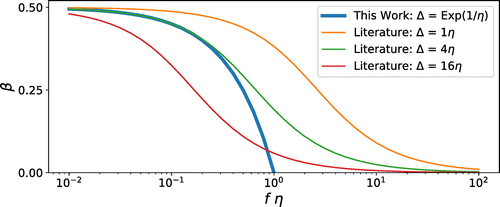
Figure 1 shows that the adversarial tolerance guarantees provided by this work with are better than the best possible guarantees with in the range . Consider, for the sake of illustration, a system such that Δ has the distribution that is identical to from and concentrates the rest of the mass at . Such a distribution is stochastically dominated by both and the constant delay ; thus, guarantees for both models apply. For such a system, the security region of the protocol as guaranteed by Theorem 1 is greater than what can be established via the synchronous model alone. This shows that explicitly accounting for random delays can provide better security guarantees than simply working with the worst-case delay.
The upper bound on the probability of a successful attack, as given in Theorem 1, decreases exponentially as a function of fk. To explore the constant in the exponent, we perform a Monte Carlo simulation of the private attack. Figure 2 shows the estimated probability of success of the attack. The simulations show an exponential decrease in the probability of a successful attack. Moreover, the plot also illustrates that the adversary’s chance of success increases with the mean delay; this trend is also reflected in Theorem 1. Comparing the bounds given in Theorem 1 to the simulation results, we observe that the constants in the exponent in our bounds are not tight. We chose to express our theorems with simple, explicit bounds, rather than bounds that require numerical optimization or sophisticated analysis. We leave it for future work to obtain numerically tighter bounds.
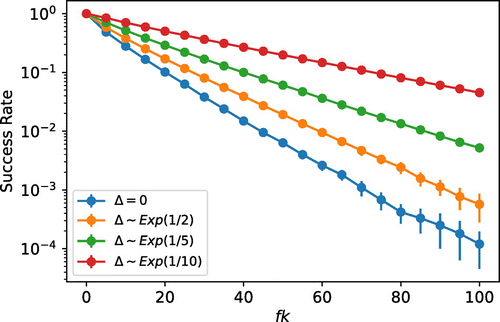
Note. The adversarial strength is , the mining rate is f = 0.1, and the delays are exponentially distributed in each setting.
3.3. Proof Sketch
The basic intuition guiding the security analysis in this work is the following. The security properties are likely to be violate if the adversary can build two equally long chains that fork far back in time. There are two factors that contribute to long forked chains, namely, adversarial blocks and network delays among honest parties. To elaborate, the adversary can purposely deviate from the longest-chain rule and use its blocks to extend the shorter of two competing chains. In addition, due to network delays, it is possible that some honest parties extend the shorter of two forked chains, simply because they have not heard of the latest block(s) on the longer chain. If the number of adversarial blocks and the number of forked honest blocks are small relative to the length of the chains of honest parties, the protocol remains secure.
To distinguish between honest blocks that grow the chain from those that do not, we introduce the notion of special honest slots. These are recursively defined such that the leader of each special honest slot has necessarily heard of the message sent by the leader of the previous slot. It immediately follows that blocks from special honest slots are always built at ever-increasing heights on the blocktree, contributing to its growth. All other honest blocks are treated as adversarial, as they could be placed arbitrarily in the blocktree. (This is one of the reasons our bounds are loose; tighter bounds on the security analysis would require a more careful analysis of all honest blocks.)
Whether a given honest slot s is special honest is determined by two random entities: the time passed since the last special honest slot, and the delay in conveying that block to the leader of s. Both these factors are beyond the adversary’s control; they depend solely on the mining rate f and the delay distribution Δ. The ϵ-honest majority condition required for security (Definition 5) is simply the requirement that every new block is special honest with probability at least a half. If this condition holds, then over any considerable interval, the number of special honest slots exceed the number of adversarial slots with high probability. We show that this is sufficient to guarantee security.
The rest of the paper is devoted to the proof of Theorem 1. Section 4 introduces some key notation and the definition of special honest slots. The proof is split into two main components. First, via a deterministic, combinatorial analysis, we obtain a sufficient condition for security, (Section 5). Second, we provide an upper bound on the probability of occurring (Section 6). Together, these results provide the desired security guarantee (Section 7).
4. Definitions of Key Random Processes
All random processes in our model are discrete-time processes, indexed by , or (the relevant indexing will be specified when the process is defined). For a random process , the notation for the ith variable is . Denote an interval of slots by . The portion of the process over such an interval is denoted by . If (and by extension, ) denotes an empty interval (or string).
4.1. as a Stationary Renewal Process
We start by defining , a random process which represents the sequence of leaders in each slot without the leader identities. We then extend this process to negative time. takes values in . For ,
is an i.i.d. process with and (see Section 2.3). Extend this process to negative time by defining to be a sequence of i.i.d. random variables with the same probabilities as noted above. Call all slots with as nonempty slots and those with as honest slots. Let denote the indices of the nonempty slots of from slot 1 onward. Similarly, let index the nonempty slots before or up to slot zero, going backward in time. For any interval , define to be the number of nonempty slots in that interval.
A random process is stationary if its distribution is invariant under any deterministic time shift. A renewal process is an arrival process (a sequence of events or arrivals) where the intervals between arrivals are i.i.d. The times of the arrivals are called renewal points, and the gap between renewal points is called the lifetime. The set of nonempty slots forms a stationary renewal process with lifetime distribution Given the locations of all the renewal points, the labels at the renewal points are i.i.d. Bernoulli random variables with . For any has distribution , whereas so that is the sum of two independent random variables minus one. In the terminology of renewal theory, is the sampled lifetime sampled at time 0. In the Ouroboros line of works (Kiayias et al. 2017, Badertscher et al. 2018, David et al. 2018), the process is called the characteristic string. We reserve that term for a slightly different process, which is defined next.
4.2. Special Honest Slots and
We now introduce a new concept called special honest slots, which can be thought of as a generalization of Δ-isolated slots from Pass et al. (2017) and David et al. (2018). Simultaneously, we also define the notion of the characteristic string, denoted by . The process is a process indexed by , taking values in . In , special honest slots are marked with symbol 0, other nonempty slots with symbol 1, and empty slots with the symbol . Thus, is obtained from , by converting some zero symbols to one (those honest slots that are not special).
The precise definition of for the one-time leader model is given in the remainder of this section. (The construction in the i.i.d. leader model is given in Appendix B.) In the construction of , consider the entire process (in particular, ) and all the previously defined quantities as given. We introduce some additional notation for convenience. For all j > 0 such that Tj is an honest slot, let hj denote the leader of the slot. Let denote the delay bound (set by the network) in the message sent by hj in slot Tj to an honest party . Finally, let be random variables with the same distribution as Δ for all honest slots .
For all such that , let . For , if , let be zero with probability , and let be one otherwise. The aforementioned choices are conditionally independent across all It remains to define for all such that slot Tj is honest. This is done sequentially. For , let denote the last special honest slot, that is, slot with strictly before Tj. Let if slot Tj is honest and , where . Otherwise, let The process for negative time was used to define the first special honest slot in positive time. This concludes the construction of , given , the identities of the honest leaders hj, and the delay bounds among all honest parties . All these are random entities, not controlled by the adversary. Later, in Section 6.2, we characterize the distribution of . In particular, it is a stationary process, a property that is useful in our security analysis.
Special honest slots are the slots Tj where . Those nonempty slots that are not special honest are defined to be adversarial. This includes those slots that are honest, but not special honest. Define the blocks that are created by the leaders of special honest slots to be special honest blocks.
For any interval , define to be the number of special honest slots, and let denote the number of adversarial slots, in that interval. It follows that Special honest slots have the following key property: blocks created in successive special honest slots are built at strictly increasing heights. Note that hj receives the message from the previous special honest slot at or before time . If Tj is special honest, then Thus, the condition for Tj to be a special honest slot is sufficient, but not necessary, for hj to have heard of the message from the previous special honest slot. From this, the aforementioned property follows. This property is used to lower bound the length of the portion of chains in Lemmas 3 and 4. It is also used in Lemma 5 to derive a necessary condition for consistency violation.
4.3. The Process
For an honest party h and let denote the special honest slot with greatest index such that the broadcast in that slot must have been heard by h by the end of slot i (even if the adversary maximally delays the messages). That is,
We use the convention that the maximum of an empty set is zero. Thus, .
Let denote the number of special honest slots in the interval . In other words,
The interpretation here is that is an upper bound on the number of consecutive special honest slots that party h has not heard the messages from by slot i, counting backward from i. (It is an upper bound because it’s defined in terms of the delay upper bounds, not the true delays.) For example, means that by the end of slot i, h might not have heard the messages from the last two special honest slots occurring before or at i but it either must have heard the message sent in the third most recent special honest slot before slot i or there were only two special honest slots during Looking ahead, is used to lower bound the length of the chain , as shown in Lemma 4. In turn, this lower bound is used to derive necessary conditions for consistency and chain quality violation in Lemmas 5 and 6.
Finally, given a set of honest parties , let
5. Lemmas on Deterministic Properties
This section derives a necessary condition for the consistency property and the chain quality property to be violated. The necessary conditions for both the security properties turn out to be identical. The condition is expressed as an inequality in terms of the and processes. This inequality must hold if the adversary has violated the security properties. It can be worded as follows: over some sizable interval, the number of nonspecial honest blocks must exceed the number of special honest blocks, barring a term of (see (7) for the exact condition). In deriving this necessary condition, we factor out the arbitrary actions of the adversary; equivalently, we consider the worst-case adversarial actions. With this analysis, the proof of Theorem 1 is reduced to bounding the probability of an event concerning the random processes and .
Before formally proving these reductions, we introduce the notion of the latest special honest chain (at slot i), and use this notion to give two forms of the chain growth property. Such a property has been used by other works that analyze PoW blockchains (Garay et al. 2015, Pass et al. 2017) in their security analysis.
(Latest Special Honest Chain). For any slot , let denote the chain broadcast by the leader of the last special honest slot at or before slot i. Call this the latest special honest chain at slot i. In is the longest chain that ends in a special honest block. is the genesis block.
Two simple facts follow immediately from the definition. First, if i is a special honest slot, then is the chain that is broadcast by the leader of slot i. Second, if a chain contains a block created in a special honest slot s, then . These facts are used frequently in the following proofs. The following chain growth lemma is also easily proven.
(Chain Growth–Special Honest). Between any two time slots such that , the increase in the length of the latest special honest chain is bounded below by the number of special honest slots in the interval . I.e.,
The property of special honest slots implies that the chains broadcast in successive special honest slots must have strictly increasing lengths. This implies (6). □
As it stands, the prevous lemma only lower bounds the growth of latest special honest chains, . However, it is useful in bounding the chain growth of any honestly held chain, as shown next.
(Chain Growth–Honest). For any and any , suppose contains a special honest block created in slot r, or let r = 0. Then
Equivalently,
By the definition of (Section 4.3), the honest party h must have heard of the chain by slot i, where . Therefore, the chain it holds at slot i must be at least as long as , that is, By Lemma 3, provided . We know that (by (5)). Putting the previous inequalities together, we get
This proves the first statement, under the condition . If l < r,
Under this condition, the lemma is trivially true: must be at least as long as , as it contains the block created in slot r.
The second statement can be obtained from the first, as follows. Observe that , and therefore
The remainder of this section shows that if either the consistency or the -intensive chain quality is violated, then the event must occur, where
The analysis for the consistency property is given in Section 5.1 and that for the chain quality property is given in Section 5.2. The two analyses have a similar outline. First, the chain growth properties (Lemmas 3 and 4) are used to lower bound the length of a certain portion of a chain, namely . Next, the fact that the consistency (or chain quality) property is violated is used to upper bound the same quantity with the number of adversarial blocks created in that interval, . These bounds give us the lower bound on as stated in (7).
5.1. Consistency Violation Condition
Recall, from Definition 1, that the consistency property with parameters and holds in an execution if the following event occurs:
As such, if the property is violated, it implies that at two (possibly) different points in time (i, ), two honest parties held different chains. It is more convenient to argue in terms of events that are more local in time. To this end, define the event:
From (8), it follows that
states that honest parties in agree with each other at slot i, and with themselves across slots i and i + 1. If occurs for all slots , then all parties in agree with each other from slot s + k onward. This can be shown by induction on i. Therefore,
We now have all the ingredients to prove a necessary condition for consistency violation.
(Consistency Violation–Necessary Condition). Suppose, in an execution, the consistency property with parameters is violated (i.e., occurs). Then, for some r < s and ,
Suppose occurs. Then, by (10), there exists such that occurs. Therefore, it suffices to show that the event implies (11) for some r < s. By (9), implies one of two events: either there are two different honest parties that have disjoint chains at slot i, or the same honest party has disjoint chains at slot i and i + 1. The arguments for both cases are presented together; they are very similar.
In the first case, let , and assume, without loss of generality, that . In the second case, let be and be . Here too, , as the following argument shows. In slot i + 1, party h must have adopted a new chain; otherwise, consistency would not be violated. This new chain () must be strictly longer than the chain it held at slot i (, i.e., C1). Because is shorter than by at most one block, it follows that .
In both cases, and are disjoint onward from slot s or before. Put differently, all blocks on the common prefix of and are created strictly before slot s. Let r be the slot of the last special honest block in the common prefix of and . Similarly, define to be the slot of the last block in the common prefix of and . In general, , with equality holding if and only if the last common block of and is special honest.
Keeping the definitions of r and in mind, note that contains only adversarial blocks, which implies . Moreover, observe that for every block on , there is a different block on at the same height. Consider a pair of blocks at the same height, one each on and . Between these blocks, at least one must be adversarial, because two special honest blocks can never be at the same height on the blocktree. Therefore, . Putting these inequalities together gives
Recall that for any . Using this fact along with Lemma 4 gives a lower bound for :
Together, the upper and lower bounds for lead to (11):
We have proven that consistency violation implies (11) holds for some r < s and . This, in turn, implies occurs. In defining , we have allowed for the possibility of r = s as well to include chain quality violation within the same event. □
5.2. Chain Quality Violation
The necessary condition for the chain quality property to be violated is identical to that of the consistency property begin violated, and the analysis has a similar flavor as well.
(Intensive Chain Quality Violation–Necessary Condition). Suppose, in an execution, the -intensive chain quality property is violated. Then, for some and ,
Consider an execution where the intensive chain quality with parameters s, k, and is violated. This means that for some honest party and , there are no special honest blocks in . Let be chosen such that is a maximal portion of the chain without any special honest blocks. Thus, r is the slot of the last special honest block on the portion of the chain , or zero if there is no such block. In either case, . Similarly, if the portion of the chain contains at least one special honest block, then i + 1 is the slot of the first such block; else, . We know that all blocks in must be adversarial blocks, created in the interval . Therefore, To prove the lemma, it thus suffices to show
The proof of (12) is divided into the cases and
(). In this case, we know that i + 1 is a special honest slot, and the block created in that slot is part of the chain . This implies the following facts:
. Moreover, .
.
Also, . Using these facts, we get
The previous inequality follows from Lemma 3. This implies (12), as is always nonnegative.
() In this case, (12) follows immediately from the second statement of Lemma 4. □
5.3.
We conclude this section by introducing the notion of , which allows us to reformulate in a way that is easier to analyze.
(Reach). Let , and for any , let
In the previous definition, are zero because the interval is empty. Thus, is a random process that is a function of and it takes values in .
The Ouroboros line of works Kiayias et al. (2017), David et al. (2018), Badertscher et al. (2018), and Blum et al. (2020) define as an upper bound on the extent to which an adversarial chain can “reach” beyond any honest chain in the blocktree . The two definitions can be shown to be equivalent. With this definition in place, we can rewrite as
This can be proved by first splitting as (and likewise for ), and then noting that for any value x,
The remaining paper is devoted to finding a bound on .
6. Lemmas on Probabilistic Properties
Consider the expression of in (13). To bound , we need to bound the three terms and . The first two terms should be viewed as processes, that is, functions of i. These processes need to be bounded for all time (beyond slot s + k). To obtain such bounds, we work with compressed versions of these processes, obtained by sampling them at nonempty slots alone. Section 6.1 defines the necessary terms and results to perform this mapping between time scales. Sections 6.2, 6.3, and 6.4 analyze the distribution of the processes , and , respectively. The results of this section are combined to give an upper bound on in Section 7.
6.1. Reduction to Compressed Time Scale
Define a new time scale driven by the arrival of nonempty slots: The clock ticks by one whenever a new nonempty slot occurs. Call this event-driven time scale the compressed time scale. The following notation is used to define the processes and on the compressed time scale. For and , let
In other words, is the nonempty slot strictly after time s. Clearly, . For any and the random variables are i.i.d. with distribution Let denote the time-shifted, compressed version of relative to reference slot s:
and , which are the compressed versions of and respectively, are also defined in a similar manner. Finally, let and be time-shifted, compressed versions of and respectively. Specifically,
is defined similarly. We now state the main result of this section.
Given , let
Then, the event satisfies , which implies
First, both and , as functions of i, are constant over intervals of the form . Second, the process is nonincreasing over such intervals. This is because only increases at special honest slots. Now, suppose the event holds. If j is such that is the last renewal time less than or equal to i, then
If F0 does not hold, then . This implies that , and hence F1 is true. This completes the proof of the first claim. This claim implies that is bounded above by . This, by the union bound, is bounded above by . This shows the second claim. □
The following lemma, proven in Appendix A, Section A.1, gives a bound on , that is,
Suppose such that Then
The results in the following subsections are used to bound .
6.2. On
The main result of this subsection, Lemma 9, characterizes the distribution of . In essence, it specifies how to construct a process with identical distribution to . First, generate a stationary renewal process on with lifetime distribution At all slots except the renewal points, set the symbol to . Let the renewal points be indexed by . At each renewal point j, set the symbol to zero with probability and to one otherwise, and do so independently for every renewal point; here, gj is the gap between the jth and renewal point. Here, we give the proof for the one-time leader model. The identical statement for the i.i.d. leader model is proven in Appendix B.
(Distribution of ). The sequence of nonempty slots, forms a stationary renewal process with lifetime distribution Conditioned on the random variables are independent and Bernoulli with the following distribution:
In particular, is a stationary process.
The first claim is already established in Section 4.1; it follows from the distribution of . The second claim is true for by construction, as shown in Section 4.2. We now show the second claim for . Recall, from Section 4.2, if and , where Rj is the delay from the last special honest slot before Tj to hj. The sequence is a Bernoulli process with probability of zero being α. Moreover, it is independent of the sequence . It therefore suffices to show that given , the sequence of random variables are i.i.d. with the same distribution as Δ.
The last statement can be shown in three steps. First, given , the message delays are mutually independent with the same distribution as Δ. Second, the sequence is a subset of all the delay random variables, and whether a delay variable is in this sequence or not is independent of its value. Third, as a consequence of the one-time leader model, each Rj represents a different message’s delay. This is because the recipient hj is always different, even if the sender may be the same for different js.
The fact that the nonempty slots form a stationary process with independent lifetimes, together with the fact that the value of at the nonempty slots is determined by the immediate lifetime, implies that is a stationary process. □
From Lemma 9, we get the following result, which states that the process is nearly a Bernoulli process, and in fact, can be stochastically dominated by one.
(Distribution of ). For any ,
Furthermore, for any and ,
Here, is the parameter defined in Definition 5, and denotes the portion of indexed by .
By the stationarity of (from Lemma 9), it suffices to prove the lemma for s = 0. The desired result follows from Lemma 9 and carefully arguing about conditional probabilities.
Pick any . Lemma 9 implies the following: If we condition on and , the conditional probability of is . Now consider taking out Tj from the conditioned variables. In other words, restrict the information being conditioned on to and . The conditional probability of is now , where is independent of Δ.
If has the lifetime distribution, . Thus, the conditional probability above is simply p. For j = 1, has the sampled lifetime distribution, which is the sum of two independent random variables minus one (see Section 4.1). This distribution stochastically dominates the distribution. Therefore, the conditional probability above is lower bounded by p. Finally, is a deterministic function of the sequences and . Therefore, the statements of the lemma follow. □
The last result of this section gives a bound on the process . It states that the process eventually remains below a line whose slope is greater than its drift. The result is proven in Appendix A, Section A.2.
For any ,
6.3. On
The main result of this section, Lemma 12, states that the marginal distribution of both and are stochastically dominated by a geometric distribution with an appropriate parameter. The statement is easy to foresee through the following understanding. A given honest party h is sent a fresh new message at every special honest slot. Therefore, has the interpretation of the number of consecutive failed trials until the first success; here, each trial corresponds to a different special honest slot and success implies the message from that special honest slot being heard by slot i. These trials are independent. By upper bounding the probability of failure away from one, we obtain a geometric bound on .
(Distribution of Unheard). Let The following statements hold:
(a) For any for all integers
(b) For any for all integers
Fix It is possible that i itself is a special honest slot and h has not heard it by slot i. In any case, is less than or equal to one plus the number of consecutive special honest slots from strictly before slot i that h has not heard by slot i. The nonempty slots form both a Bernoulli process with parameter f and a renewal process. Let denote the lifetimes of the renewal process going backward from slot i. Thus, is the nonempty slot before i. The random variables Di are independent with the distribution.
The last special honest slot before slot i must be at least D1 slots before slot i, so the probability h has heard that special honest slot is at least q. In general, for , the from the last special honest slot before slot i must be at least Dj slots before slot i. (Here Dj is used as a lower bound on ) Thus, no matter which of the last j − 1 special honest slots before slot i that h has heard, the probability h hears the from last special honest slot before i is at least q. Therefore, can be viewed as at most one plus the number of consecutive failures in a sequence of trials, such that each successive trial is successful with probability at least q. Thus, is stochastically dominated by the distribution, which is the conclusion of (a).
The proof of (b) is obtained in a similar fashion by replacing i with , for a fixed and There is just one subtlety that we note here. If we consider the renewal process from the perspective of slot which is the renewal point after slot s, the lifetime going backward has the sampled lifetime distribution; all the other lifetimes have the distribution. The sampled lifetime distribution is equivalent to the sum of two independent random variables minus one, and is stochastically greater that the typical lifetime distribution, Thus, the arguments in the proof of (a) continue to hold. Importantly, these lifetimes are mutually independent. □
Lemma 13, proven in Appendix A.3, follows from the above result and the union bound.
For any and c > 0,
6.4. On
In this section, we show that the distribution of has a geometric tail. From Definition 7, it follows by induction on i that satisfies the following recursion:
The initial condition of the recursion, , is given in Definition 7 itself.
Next, define to be the backward residual lifetime process for the locations of the nonempty slots in , counting from zero. Mathematically,
The next lemma characterizes the joint process . The proof is given in Appendix A.4.
The process is a discrete-time Markov process with equilibrium probability mass function given by
In other words, under the equilibrium distribution, is independent of has the distribution and has the distribution.
This result gives us a handle on the marginal distribution of , as shown here.
(Distribution of Reach). For all .
The initialization of is Consider a comparison system such that is a random variable independent of with the distribution. Then in the comparison system, is a stationary Markov process, and in particular, has the distribution for all i. Now, for fixed, all the variables are nondecreasing functions of the initial state , as can be readily shown by induction on i. Because the actual initial state of the original system is less than the initial state of the comparison system, it follows that in the original system is stochastically dominated by the distribution. □
7. Proof of Theorem 1
Theorem 1 provides an upper bound on the probability that either consistency or intensive chain quality is violated in an execution. In Section 5, we showed that if either security property is violated, then must necessarily occur. Furthermore, Lemma 7 shows that for appropriately defined events F0 and F1. Thus, to prove Theorem 1, it suffices to show
By Lemma 8, for any ,
Recall from Lemma 7 that
Consider the following bounds on the terms that appear in the expression of F1:
The first bound follows from Lemma 11 (replace c by ϵc), the second from Lemma 13 (replace b by and c by ϵc), and the third from Lemma 15 (replace a by and use the fact that ). Here, a, r, and c are free parameters belonging to the set (0, 1) and . By the union bound, (19), (20), and (21) give the following result:
In obtaining this bound, we use the following fact: for three discrete terms x, y, z, the condition implies either , or . We also use the fact that is the maximum of for all .
With bounds on F0 and F1 (namely, (18) and (22)), it remains to set the free variables. Let and a = 1/8. This implies . Also use the fact that (see Lemma 12 for q). Last, use the bound , which follows from for . The previous steps show that (17) holds for
This concludes the proof of Theorem 1.
Appendix A. Proofs of Lemmas in Section 6
A.1. Proof of Lemma 8
(Restated from Main Text). Suppose such that Then .
Note that and has the binomial distribution with parameters k and f. Thus,
Here, we use the bound □
A.2. Proof of Lemma 11
Let denote a simple integer valued random walk with a drift , where In other words, and
The aim of this section is to prove Lemma 11, which we restate here.
(Restated from Main Text). For any ,
For any , Lemma 10 implies
Moreover, the same lemma implies is stochastically dominated by , because the former has value zero at j = 1 with probability greater than p. Thus, to prove the lemma, it suffices to show that the same bound holds for instead of .
For any , for any ,
Let to be determined below. Observe that the event on the left-hand side of (A.2) is contained in where and
is the sum of k i.i.d. random variables with zero mean, each taking values in an interval of a length of two. Therefore, Hoeffding’s inequality implies that for any , . Setting yields
Let Y be a random variable such that
To obtain a bound on Hoeffding’s lemma for bounded random variables (Hoeffding 1963) implies that . Taking shows that Therefore, Thus, for any ,
For any , the random processes and have the same distribution. Therefore, (A.3) implies
Thus, Setting gives . Using yields
A.3. Proof of Lemma 13
(Restated from Main Text). For any and c > 0,
Lemma 12(b) implies
Substituting for t and using the union bound by summing over the possible values of implies that the left-hand side of (13) is bounded from above by
Using the inequality , the bound in Equation (13) follows. □
A.4. Proof of Lemma 14
(Restated from Main Text). The process is a discrete-time Markov process with equilibrium probability mass function given by
In other words, under the equilibrium distribution, is independent of has the distribution and has the distribution.
The Markov property follows from
The nonzero transition probabilities out of any given state are given by (with ):
To verify π is the equilibrium distribution, it suffices to check that if the state of the process at one time has distribution π, then in one step of the process, the probability of jumping out of any given state is equal to the probability of jumping into the state. For a state of the form (b, r) with , the probability of jumping into the state is which is equal to the probability of jumping out of the state. For a state of the form with , the probability of jumping into the state satisfies the following:
Appendix B. for the i.i.d. Leader Model
In this section, we give the precise construction of for the i.i.d. leader model, show that it implies the property of increasing heights of special honest blocks, and prove Lemma 9 for this construction. All other properties of follow from these. Before starting, we briefly describe a possible scenario that makes the i.i.d. model more complicated than the one time leader model. Suppose a special honest party hA transmits a message in some slot i, and the next two slots an honest party is elected in are slots j1 and j2 and the same honest party hB is elected in both j1 and Furthermore, suppose hB has not heard the message sent by hA before slot j1, so that slot j1 is not a special honest slot. Then we need to consider the conditional probability that hB has heard the message from hA before slot given the message was not received before slot If the delay distribution has a heavy tail, in particular if infinite delays are allowed, then the conditional distribution of residual delay given that the delay is greater than or equal to could be much different from the unconditional distribution.
B.1. Internal Representation and Refreshed Residuals
The definitions in this section are used in the following to define special honest slots for the i.i.d. leader model. Consider a probability mass function (pmf) p on The failure rate function, aka hazard rate function, of the pmf, p, is defined by
A random variable D with pmf p can be constructed as follows. Let , where is a sequence of independent random variables that are each uniformly distributed on the interval . We call the internal representation of D. If D1 and D2 are random variables with independent internal representations, then D1 and D2 are independent as well.
Given , define the refreshed residual of D at elapsed time d by Although depends on the internal representation of D, the internal representation is suppressed in the notation.
Let D be a -valued random variable with an internal representation and let The following hold.
(a) .
(b) The random variable is independent of . More generally, if , then and are mutually independent.
(c) If D has a nondecreasing failure rate function,
Statement (a) follows from The first statement in (b) follows from the facts that is determined by and is determined by . The generalization in (b) similarly follows: the indicated random variables are functions of disjoint subsets of the random variables in . (c) is proved as follows.
The nondecreasing failure rate condition is used in the second inequality. □
B.2. Defining
In this section, we define in the i.i.d. leader model. Without loss of generality, we assume all message delays have independent internal representations. The definition of is the same as in the one-time leader model except for the way in which special honest slots are defined in positive time. In particular, the variables Rj are defined differently. For each such that , let
Just as before, Tj is a special honest slot (i.e., ) if and only if and When (i.e., the latest nonempty slot was special honest), . Recall that this is precisely the definition of Rj in the one-time leader model. This modified definition of Rj allows us to prove Lemma 9 even if the sequence of Rjs is not i.i.d. (see the proof given later).
Next, we show that the property of increasing heights of special honest blocks holds for the i.i.d. leader model as well. Note that hj receives the message from the previous special honest slot at time . If Tj is special honest, then By Lemma B.1(c), . Put together, we get
Thus, just as for the one-time leader model, the condition for Tj to be a special honest slot is sufficient, but not necessary, for hj to have received the message from the previous special honest slot.
The final step is to show that the distribution of the random process for the i.i.d. leader model is the same as it is for the one time leader model.
(Distribution of ; Restated from Main Text). The sequence of nonempty slots, forms a stationary renewal process with lifetime distribution Conditioned on the random variables are independent and Bernoulli with the following distribution:
In particular, is a stationary process.
It suffices to show the second claim for ; all other statements follow from identical arguments as in the one-time leader case. Recall that if and only if and . Consider the conditional probability distribution of the sequence given Statements (a) and (b) of Lemma B.1 imply that, given ,
Each Rj has the same distribution as Δ and
The random variables are conditionally mutually independent.
Next, if and only if . Finally, the sequence () is a Bernoulli sequence. From these observations, the conditional independence of follows and so does the equation in the lemma. Thus, we have shown the second claim holds for . □
References
- (2018) Ouroboros genesis: Composable proof-of-stake blockchains with dynamic availability. Backes M, Wang XF, eds. Proc. ACM SIGSAC Conf. on Computer and Comm Security (Association for Computing Machinery, New York), 913–930.Google Scholar
- (2019) SoK: Consensus in the age of blockchains. Abraham I, Eyal I, Gün Sirer E, eds. Proc. 1st ACM Conf. on Advances in Financial Technologies (Association for Computing Machinery, New York), 183–198.Google Scholar
- (2020) The combinatorics of the longest-chain rule: Linear consistency for proof-of-stake blockchains. Chawla S, eds. Proc. 14th Annual ACM-SIAM Sympos. on Discrete Algorithms (Society for Industrial and Applied Mathematics, Philadelphia), 1135–1154.Google Scholar
- (2018) Ouroboros praos: An adaptively-secure, semi-synchronous proof-of-stake blockchain. Nielsen JB, Rijmen V, eds. Annual Internat. Conf. on the Theory and Appl. of Cryptographic Techniques (Springer International Publishing, Cham, Switzerland), 66–98.Google Scholar
- (2013) Information propagation in the bitcoin network. Lo Cigno R, Felber P, Iamnitchi A, eds. Proc. IEEE P2P (Institute of Electrical and Electronics Engineers, New York), 1–10.Google Scholar
- (2020) Everything is a race and nakamoto always wins. Katz J, Vigna G, eds. Proc. 2020 ACM SIGSAC Conf. on Computer and Comm. Security (Association for Computing Machinery, New York), 859–878.Google Scholar
- (1988) Consensus in the presence of partial synchrony. J. ACM 35(2):288–323.Google Scholar
- (2019) Barracuda: The power of l-polling in proof-of-stake blockchains. Subramanian V, Yi Y, eds. Proc. 20th ACM Internat. Sympos. on Mobile Ad Hoc Networking and Comput. (Association for Computing Machinery, New York), 351–360.Google Scholar
- (2020) SoK: A consensus taxonomy in the blockchain era. Jarecki S, ed. Proc. Cryptographers’ Track at the RSA Conf. (Springer International Publishing, Cham), 284–318.Google Scholar
- (2015) The bitcoin backbone protocol: Analysis and applications. Oswald E, Fischlin M, eds. Annual Internat. Conf. on the Theory and Appl. of Cryptographic Techniques (Springer International Publishing, Cham, Switzerland), 281–310.Google Scholar
- (2020) Tight consistency bounds for bitcoin. Katz J, Vigna G, eds. Proc. ACM SIGSAC Conf. on Computer and Comm. Security (Association for Computing Machinery, New York), 819–838.Google Scholar
- (2022) Practical settlement bounds for proof-of-work blockchains. Cremers C, Shi E, eds. Proc. ACM SIGSAC Conf. on Computer and Comm. Security (Association for Computing Machinery, New York), 1217–1230.Google Scholar
- (2019) Fraud risk assessment within blockchain transactions. Adv. Appl. Probability 51(2):443–467.Google Scholar
- (2020) Stability and scalability of blockchain systems. Proc. ACM Measures and Analysis of Computer Systems (Association for Computing Machinery, New York), 35.Google Scholar
- (1963) Probability inequalities for sums of bounded random variables. J. Amer. Statist. Assoc. 58:13–30.Google Scholar
- (2017) Ouroboros: A provably secure proof-of-stake blockchain protocol. Shacham H, Katz J, eds. Annual Internat. Cryptology Conf. (Springer International Publishing, Cham, Switzerland), 357–388.Google Scholar
- (1964) A martingale inequality in the theory of queues. Cambridge Philosophical Soc. 59:359–361.Google Scholar
- (2021) Close latency–security trade-off for the Nakamoto consensus. Baldimtsi F, Roughgarden T, eds. Proc. 3rd ACM Conf. on Adv. in Financial Technologies (Association for Computing Machinery, New York), 100–113.Google Scholar
- (2008) Bitcoin: A peer-to-peer electronic cash system. Accessed October 31, 2008, https://bitcoin.org/bitcoin.pdf.Google Scholar
- (2021) Ebb-and-flow protocols: A resolution of the availability-finality dilemma. Oprea A, Holz T, eds. Proc. IEEE Sympos. on Security and Privacy (IEEE, New York), 446–465.Google Scholar
- (2017) The sleepy model of consensus. Takagi T, Peyrin T, eds. Proc. Internat. Conf. on the Theory and Appl. of Cryptology and Information Security (Springer International Publishing, Cham, Switzerland), 380–409.Google Scholar
- (2017) Analysis of the blockchain protocol in asynchronous networks. Coron J-S, Nielsen JB, eds. Proc. Annual Internat. Conf. on the Theory and Appl. of Cryptographic Techniques (Springer International Publishing, Cham, Switzerland), 643–673.Google Scholar
- (2019) Analysis of Nakamoto consensus. Preprint, submitted August 19, 2019; last revised May 18, 2020, https://eprint.iacr.org/2019/943.Google Scholar
- (2014) Analysis of hashrate-based double spending. Preprint, submitted February 9, https://arxiv.org/abs/1402.2009.Google Scholar
- (2015) Secure high-rate transaction processing in bitcoin. Böhme R, Okamoto T, eds. Proc. Internat. Conf. on Financial Cryptography and Data Security (Springer International Publishing, Cham, Switzerland), 507–527.Google Scholar

